On the -attractor T-models
Abstract
We carry out a fully analytical study of the phenomenology of -attractor T-models defined by the potential . We obtain expressions for the number of e-folds during inflation in terms of the scalar spectral index and independently in terms of the tensor-to-scalar ratio . From these expressions we obtain exact solutions for both and in terms of along with their expansions for large , in full agreement with known expressions. Eliminating the parameter from the model in terms of and we can obtain exact solutions for in terms of and which allows us to reproduce, in particular, numerical solutions presented by the Planck Collaboration for the monomial potentials. We explicitly show how these solutions are contained in the solutions for the -attractors and are also the end points of these. Finally, by also eliminating the global scale in terms of the observables and we show how in the appropriate limit the -attractor potential exactly reduces to the monomials potential. We also briefly show that for -attractor E-models, which generalize the Starobinsky potential in the Einstein frame, a similar transition occurs.
1 Introduction
In recent years alpha attractor-type models have captivated considerable attention mainly due to the fact that they have a fairly well-understood origin in conformal and super-conformal field theories as well as their close relationship with supergravity theories [1]-[15], the fact that they connect with well known monomial potentials and most importantly, because they have a phenomenology [6] that is fully consistent with reported results by e.g., the Planck Collaboration [16]. Important properties of -attractors have been extensively discussed in the literature (for a sample of articles in the subject see e.g., [17]-[33] and references therein). The resulting class of potentials generalized from the simplest monomials is of the form
| (1.1) |
and
| (1.2) |
Connecting with the original notation for T-models or for E-models thus, -attractors. These potentials can be considered on its own as phenomenological potentials for inflation and as such have also been studied, mainly numerically. The main purpose of this work is to provide a fully treatment, which can be considered as complementary to phenomenological results briefly presented in the literature [6], of the most important properties of the T-type -attractors defined by the potential (1.1).
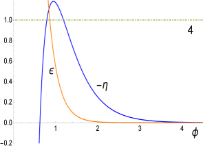
The organization of the article is as follows: In Section 2 we discuss in detail the end of slow-roll either with the condition or with where and are the usual slow-roll parameters given by [34]
| (1.3) |
is the reduced Planck mass which we set equal to 1 in most of what follows and primes on denote derivatives with respect to the inflaton field . We provide expressions for the number of e-folds from the time scales left the horizon at wavenumber mode corresponding to to end of inflation at . The expression for when is exclusively dependent on the spectral index , the model characterized by and the parameter appearing in the potential. This is done by obtaining from the equation [34]
| (1.4) |
written in the form , where is defined as . When we obtain the number of e-folds during inflation exclusively dependent on the tensor-to-scalar ratio , and by solving for from the equation
| (1.5) |
written in the form In this way we can obtain exact solutions for and for as well as their asymptotic behavior in various situations, mainly for large number of e-folds . In Section 3 we also obtain an expression for but this time in terms of , and by eliminating the parameter in terms of and . In this case we can write any quantity of interest exclusively in terms of the observables and , the quantities so written will keep tightening as more precise determination of the observables is achieved.
Using the allowed range of we can deduce the range for . In particular we find solutions for that allow us to study the - plane for various values of and . Using an approximation for in the large limit we find bounds for as well as a lower bound for the parameter . We explicitly show how the predictions for of the monomials potential are exactly contained in the solutions for of the -attractor models and should also be the ending points of the curves [6]. To fully clarify this phenomenon we also determine the global scale in terms of and through the equation
| (1.6) |
Thus, a direct study of the potential (1.1) with and eliminated in terms of and shows how it transitions exactly to the monomials potential in the limiting case in which the relationship between the observables and of the monomials is fulfilled and we illustrate graphically this phenomenon in Fig. 11. We show briefly that this is also the case for the type of E-models (1.2) that can be considered as generalizations of the Starobinsky model in the Einstein frame (see Fig. 12). Finally, Section 4 contains our conclusions on the main points discussed in the article.
2 The -attractor T-models
The -attractor T-models generalized from the simplest monomials are defined by the potential given by Eq. (1.1), where is a positive number which distinguishes among the models and is a parameter. When necessary we can understand in Eq. (1.1) as its absolute value to guarantee a bounded potential from below. We do not write it explicitly anywhere because we will be working in the positive region of always unless stated otherwise. An expression for , the inflaton at horizon crossing, is obtained by solving Eq. (1.4), , with the result
| (2.1) |
where is defined as . For large the end of slow-roll is given by the solution to the equation while for small by the condition . The value of which solves the condition is and it is given by
| (2.2) |
while the solution for the case is
| (2.3) |
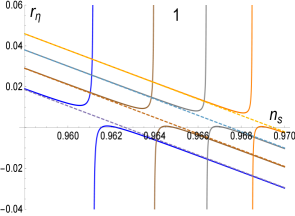
The solution Eq. (2.2) makes sense for . Thus, the value of which separates one -solution from the other is obtained by solving with the result (see Fig. 1)
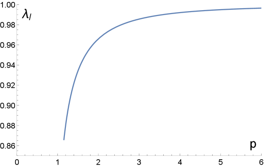
| (2.4) |
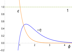
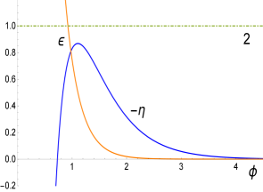
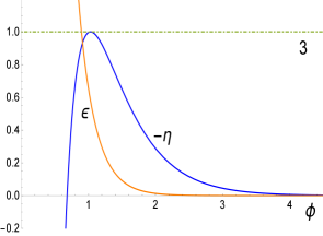
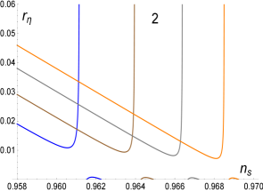
whenever . The value of signals the minimum value can have (for a given when (see Fig. 2, in particular panel number 3). Thus, for the end of inflation is dictated by the condition while the case requires solving the equation for the end of slow-roll with the solution given above. For , .
The number of e-folds from the time scales the order of the pivot scale left the horizon during inflation at to the end of inflation at is given by
| (2.5) |
We can write in the form where
| (2.6) |
and
| (2.7) |
2.1 Slow-roll interruptus
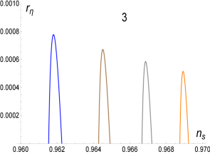
An interesting phenomenon occurs near the end of inflation and we illustrate it below for the case . By looking at the third panel in Fig. 2 (in Fig. 2 we plot ) we see that the curve just touches the horizontal line at 1 for . This means that the condition has been marginally satisfied signaling the end of slow-roll. In the Fig. 3 this detail is amplified together with a second curve for corresponding to a value slightly greater than (). We can see that at the point the condition is saturated but the curve enters again the region at when is still less than 1 i.e., slow-roll resets to eventually end inflation at when is finally equal to one.
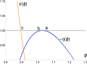
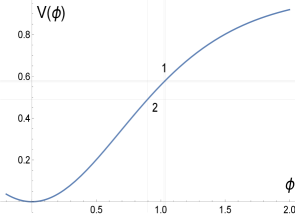
In Fig. 3 we also show the potential for during this phenomenon: the small box under the number 1 in Fig. 3 shows the region during which slow-roll has ended and in the square above 2 the region where slow-roll is restored to eventually end permanently in the l.h.s. corner of the square corresponding to . The total number of e-folds between points and is corresponding to an increase of the size of the universe in . For slightly higher values of slow-roll will be interrupted for a longer period. While the number of e-folds after slow-roll is restored is negligible, the phenomenon itself is interesting and worth reporting.
2.2 The case
The equations for and , Eqs. (2.6) and (2.7) respectively, are obtained by substituting and from (2.1) and (2.2). Together with the large expansion they are given by
| (2.8) |
and
| (2.9) |
We see that both terms are -independent for infinitely large , the term associated with the end of slow-roll is negligible contributing with less than 1 e-fold. We will see in Subsection 2.3 that when is small this is not the case and is important.
Using Eqs. (2.8) and (2.9), the number of e-folds can be written in terms of the observable as follows
| (2.10) |
where and the subindex appears here to remind us that is obtained from the solution to the condition but then it is dropped (as well as the argument) from the following expressions. For large , has the following expansion
| (2.11) |
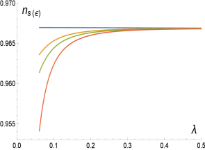
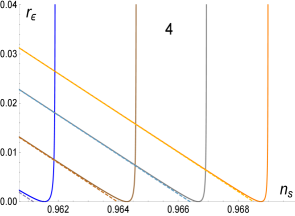
Thus, is -independent for infinitely large . We can solve Eq. (2.10) for in terms of (see Fig. 4)
| (2.12) |
Thus, the leading order term in the large- expansion of the scalar spectral index is also p-independent
| (2.13) |
One can notice that as given by Eq. (2.10) above depends only on the observable , this is so because was obtained by solving the equation (1.4) written in the form . We could also obtain by solving Eq. (1.5) or and write an equivalent expression for involving only the observable with the result
| (2.14) |
which together with Eq. (2.2) implies that the number of e-folds can now be written as
| (2.15) |
Solving for
| (2.16) |
as shown by Fig. 4 for the case and for various values of . In the large- limit is given by
| (2.17) |
2.3 The case
The end of inflation is given by the solution to the condition
| (2.18) |
while in terms of is given, as before, by Eq. (2.1).
The equations for and , Eqs. (2.6) and (2.7) respectively, and their small expansion, are given by
| (2.19) |
and
| (2.20) |
For small the first term in the expansion of grows large thus, (contrary to the large case where is less than 1) here the end of inflation is important and necessary to cancel the leading term in so that the number of e-folds of inflation goes like , to first approximation.
The number of e-folds Eq. (2.5) is
| (2.21) |
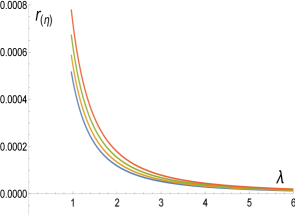
where and, in analogy with Eq. (2.10), the subindex appears here to remind us that is obtained from the solution to the condition but then it is dropped from the following expressions. From Eq. (2.21) we can solve for (see Fig. 5)
| (2.22) |
for large
| (2.23) |
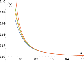
To obtain in terms of we proceed in a similar way as in Eq. (2.16). From Eqs. (2.5), (2.14) and (2.3) we get
| (2.24) |
solving for (see Fig. 5)
| (2.25) |
with large expansion
| (2.26) |
The previous results for in the large expansion Eqs. (2.13) and (2.23) give a leading term . Also Eqs. (2.17) and (2.26) give a leading term for the large expansion of .
3 Removing the and parameters
We can express the parameter purely in terms of and the observables and by substituting e.g., from Eq. (2.1) in Eq. (1.5), , and solving for
| (3.1) |
Technically, the parameter can take values from 0 to . The limiting value occurs for or, equivalently, which is exactly the relation between and for monomial potentials of the form . Clearly when .
The limiting value , defined by Eq. (2.4), distinguishes between ending slow-roll by or . For given by (3.1) above, translates into a limiting value for , for a fixed value of , as follows
| (3.2) |
thus,
| (3.3) |
When we have
| (3.4) |
the case implies for [16] . When the condition is met , and should be less than while values of larger than correspond to which occur when the condition ends inflation (see Fig. 6) thus, the condition is only satisfied for small values of . For example, for the largest value of is which occurs for while for the largest value is also at
For small , has the following expansion
| (3.5) |
thus, to leading order in , is -independent. However, from the bounds and , the parameter is bounded from below as where is the upper bound for . For the current bounds and , a lower bound for is implied as .
3.1 General solutions for
We can eliminate the parameter in all the previous equations in such a way that only the observables and appear. First we separately discuss the case by substituting from Eq. (3.1) into the expressions for given by Eqs. (2.10), (2.15), (2.21), (2.24) and solving for obtaining the following independent solutions: one for the case where the end of slow-roll is given by the condition and labeled by the symbol and one for the case where the end of inflation is given by the condition , labeled by the symbol
| (3.6) |
| (3.7) |
The approximations for large are (see Figs. 7 and 8 for the case).
| (3.8) |
| (3.9) |
For we can proceed in an analogous way as above and solving in each case for in terms of , and obtaining the following two independent solutions
| (3.10) |
where and
| (3.11) |
where . Approximations for large are as follows
| (3.12) |
| (3.13) |
We expect the first term to dominate and should be positive thus, for , while requires or, perhaps more appropriate, for , while requires . From the Planck bounds it follows that for any . For a dominant first term we also expect that where is the upper bound for reported by the Planck 2018 Collaboration [16] . Thus assuming that
| (3.14) |
we get
| (3.15) |
where is the lower bound for and is the upper bound for . The tensor-to-scalar ratio is determined at thus, we conclude that should be bigger than at the scale of wavenumber mode .
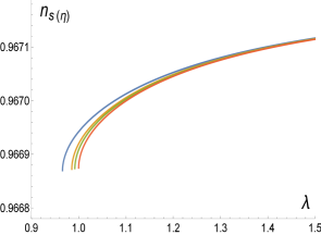
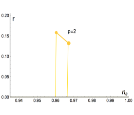
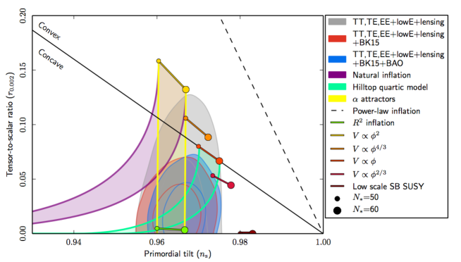
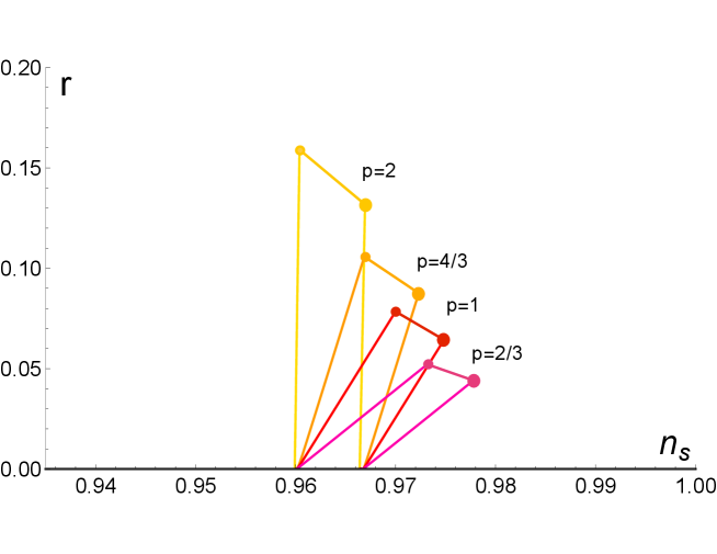
For the case, the bound is equivalent to a bound on as for . Thus, the expression for is valid for very small only. In this regime the solution (which should be used for or at ) is very close to the solution being possible to use it also for the very small regime (large regime) with negligible error. The case is not very different thus, in what follows, we study only the solution for all possible values of . In Fig. 7 we show the solutions (3.6) and (3.7) for the case reproducing in Fig. 8 the numerical solution which appear in Fig. 8 of the Planck 2018 Collaboration [16] (shown here as Fig. 9). This solution contains the monomial solution for of the model. In Fig. 10 we plot several other cases of Eq. (3.11) by giving the values and containing all the monomial solutions shown in Fig. 9. These solutions are contained exactly in the -attractor models as shown analytically in the following subsection.
3.2 Monomials as particular cases of -attractors
For monomials of the form we get and from where it follows that
| (3.16) |
also
| (3.17) |
Eqs. (3.16) and (3.17) follow from the condition , this condition ends inflation whenever . Por outside this range slow-roll is terminated by for in which case or for in this case . In any case for large and they all have the same limit . Thus for and , and so on. In this way we can calculate all the points appearing as circles in Fig. 9. The point , for example, is reached by the solution Eq. (3.7) for as shown by the left line in Fig. 8 and similarly for the line on the r.h.s. For Eq. (3.11) applies. In this way we draw Fig. 10 connecting the -attractor T-models with all the monomial as shown. Analytically, we can see this as follows: for the case we sustitute Eq. (3.17) in Eq. (3.7) and we get which is Eq. (3.16) (with ). In general (for ) substituting Eq. (3.17) in Eq. (3.11) gives
| (3.18) |
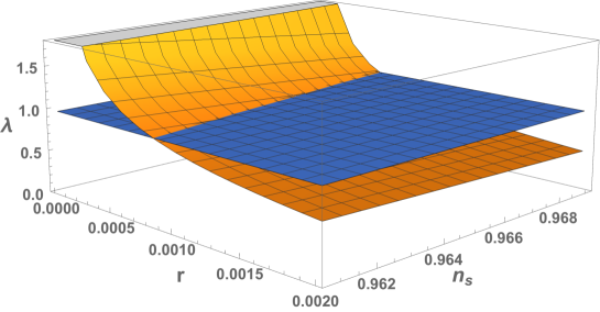
which is Eq. (3.16), exactly. Thus, all the monomial models are contained as particular cases by the -attractor T-models. This is illustrated by Fig. 10 only for the monomials shown in Fig. 8 (reproduced here as Fig. 9) of the Planck 2018 Collaboration [16] . Even more to the point: the monomials are the ending points of the attractors [6]. This can be seen as follows: if we substitute Eq. (3.17) in the equation defining (Eq. (3.1)) we find that becoming imaginary after this point. To have a clear understanding of this phenomenon let us substitute equation (3.1) for in Eq. (1.1); the resulting potential can then be written as
| (3.19) |
where has been calculated from Eq. (1.6). If we study the potential (3.19) in the limit where we find that it reduces to the following expression
| (3.20) |
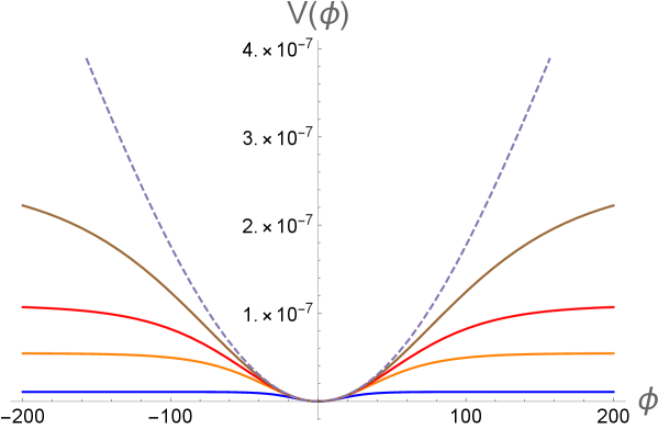
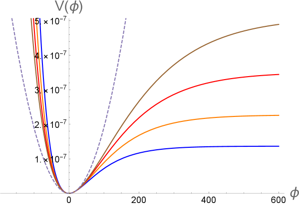
One can easily check that the potential (3.20) corresponds exactly to monomials of the form . Thus, the fact that we reach the monomials in Fig. 10 is now easily understood because our original potential transitions to the monomials potential when , that is, when which is precisely the relation between and for the monomials potential. The potential (3.19) is shown in Fig. 11 as a function of for and the mean value [16] (or ) for various values of reaching (dashed curve) signaling the transition of the potential (3.19) to the monomial potential of Eq. (3.20). The expresion makes but in what we saw before takes us to the ends of the curves in Fig. 10 reaching the predictions in the - plane for the monomials potential. A similar study can be done with -attractor E-models defined by the potential (1.2) which generalize the Starobinsky potential in the Einstein frame. In this case the generalized potential written in terms of and
| (3.21) |
also contains the monomials potential (3.20) much in the same way as discussed before (see Fig. 12).
4 Conclusions
We have carried out an analytical study of a class of -attractor T-models generalized from the simplest monomials and given by the potential without paying attention to its origin, but dealing with it only as a phenomenological model of inflation. We can see how the analytical study clarifies several of its important properties and characteristics. In particular, we have obtained exact solutions, valid for any , for the spectral index and for the tensor-to-scalar ratio in terms of the number of e-folds and the parameter . Eliminating the parameter we can also obtain exact solutions for in terms of and . These solutions allow us to study the - plane and compare with numerical studies such as those presented by the Planck Collaboration, reproducing their results. Our analytical study allows us to observe precisely how the monomial potentials are contained in the -attractor models and also constitute the end points of our solutions. Finally we show how in the appropriate limit the potential for the -attractor for both T and E-models exactly reduces to the monomials potential providing a clear explanation of the relationship between them.
Acknowledgments
I would like to thank the anonymous referee for a detailed and careful revision of the article and for useful advice. Financial support from UNAM-PAPIIT, IN104119, Estudios en gravitación y cosmología is gratefully acknowledged.
References
- [1] R. Kallosh and A. Linde. Universality Class in Conformal Inflation. JCAP, 07(2013)002.
- [2] D. Roest. Universality classes of inflation. JCAP, 01(2014)007.
- [3] S. Ferrara, R. Kallosh, A. Linde and M. Porrati. Minimal Supergravity Models of Inflation. Phys. Rev. D, 88(2013)8, 085038.
- [4] R. Kallosh and A. Linde. Non-minimal Inflationary Attractors. JCAP, 10(2013)033.
- [5] R. Kallosh and A. Linde. Multi-field Conformal Cosmological Attractors. JCAP, 12(2013)006.
- [6] R. Kallosh, A. Linde and D. Roest. Superconformal Inflationary -Attractors. JHEP, 11(2013)198.
- [7] R. Kallosh, A. Linde and D. Roest. Universal Attractor for Inflation at Strong Couplingy. Phys. Rev. Lett, 112(2014)1, 011303.
- [8] S. Cecotti and R. Kallosh. Cosmological Attractor Models and Higher Curvature Supergravity. JHEP, 05(2014)114.
- [9] R. Kallosh, A. Linde and D. Roest. Large field inflation and double -attractors. JHEP, 08(2014)052.
- [10] R. Kallosh, A. Linde and D. Roest. The double attractor behavior of induced inflation. JHEP, 09(2014)062.
- [11] M. Galante, R. Kallosh, A. Linde and D. Roest. Unity of Cosmological Inflation Attractors. Phys. Rev. Lett, 114(2014)14, 141302.
- [12] J. J. M. Carrasco, R. Kallosh and A. Linde. -Attractors: Planck, LHC and Dark Energy. JHEP, 10(2015) 147.
- [13] J. J. M. Carrasco, R. Kallosh and A. Linde. Cosmological Attractors and Initial Conditions for Inflation. Phys. Rev. D, 92(2015) 6, 063519.
- [14] J. J. M. Carrasco, R. Kallosh and A. Linde. Minimal supergravity inflation. Phys. Rev. D, 93(2016)6, 061301.
- [15] R. Kallosh and A. Linde, D Roest and T. Wrase. Sneutrino inflation with -attractors. JCAP, 11(2016) 046.
- [16] Y. Akrami et al. [Planck Collaboration], Planck 2018 results. X. Constraints on inflation. Astron. Astrophys., 641(2020) A10, arXiv:1807.06211, [astro-ph.CO].
- [17] S. D. Odintsov and V. K. Oikonomou. Inflationary -attractors from gravity. Phys. Rev. D, 94(2016)12, 124026.
- [18] Y. Ueno and K. Yamamoto. Constraining the general reheating phase in the -attractor inflationary cosmology. Phys. Rev. D, 93(2016)8, 083524.
- [19] K. S. Kumar, J. Marto, P. Vargas Moniz, and S. Das. Non-slow-roll dynamics in attractors. JCAP, 04(2016) 005.
- [20] Eshaghi, M. Zarei, N. Riazi and A. Kiasatpour. CMB and reheating constraints to -attractor inflationary models. Phys. Rev. D, 93(2016)12, 123517.
- [21] A. Di Marco, P. Cabella and N. Vittorio. Constraining the general reheating phase in the -attractor inflationary cosmology. Phys. Rev. D, 95(2017)10, 103502.
- [22] N. Rashidi, K. Nozari. -Attractor and reheating in a model with noncanonical scalar fields. Int. J. Mod. Phys. D, 27(2018) 07, 1850076.
- [23] Y. Akrami, Yashar, R. Kallosh, A. Linde and V. Vardanyan. Dark energy, -attractors, and large-scale structure surveys. JCAP, 06(2018) 041.
- [24] I. Dalianis, A. Kehagias and G. Tringas. Primordial black holes from -attractors. JCAP, 01(2019) 037.
- [25] F. X. Linares Cedeño, A. Montiel, J. C. Hidalgo and G. Germán. Bayesian evidence for -attractor dark energy models. JCAP, 08(2019) 002.
- [26] R. Shojaee, K. Nozari and F. Darabi. -Attractors and reheating in a non-minimal inflationary model. Int. J. Mod. Phys. D, 29(2020) 010, 2050077.
- [27] S. D. Odintsov and V. K. Oikonomou Inflationary attractors in gravity. Phys. Lett. B, 807(2020) 135576
- [28] R. Shojaee, K. Nozari and F. Darabi. -Attractors and reheating in a class of Galileon inflation. Int. J. Mod. Phys. D, 30(2021) 05, 2150036.
- [29] E.V. Linder. Dark energy from -attractors. Phys. Rev. D, 91(2015)12, 123012.
- [30] K. Dimopoulos, C. Owen. Quintessential Inflation with -attractors. JCAP, 06(2017) 027.
- [31] K. Dimopoulos and D. Woo. Instant preheating in quintessential inflation with -attractors. Phys. Rev. D, 97(2018)06, 063525.
- [32] C. Garcia-Garcia, E.V. Linder, P. Ruiz-Lapuente and M. Zumalacarregui. Dark energy from -attractors: phenomenology and observational constraints. JCAP, 08(2018) 022.
- [33] Y. Akrami, S. Casas, S. Deng, V. Vardanyan. Dark energy from -attractors: phenomenology and observational constraints. JCAP, 04(2021) 006.
- [34] David H. Lyth and Antonio Riotto. Particle physics models of inflation and the cosmological density perturbation. Phys. Rept., 314:1–146, 1999.
- [35] P.A.R. Ade et. al. BICEP2, Planck Collaboration. Joint Analysis of BICEP2/ and Data. Phys. Rev. Lett, 114(2015)101301.