On symmetric solutions of the fourth $q$ -Painlevé equation

Nalini Joshi School of Mathematics and Statistics F07, University of Sydney, NSW 2006 Australia [email protected] and Pieter Roffelsen [email protected]

Abstract.

The Painlevé equations possess transcendental solutions $y(t)$ with special initial values that are symmetric under rotation or reflection in the complex $t$ -plane. They correspond to monodromy problems that are explicitly solvable in terms of classical special functions. In this paper, we show the existence of such solutions for a $q$ -difference Painlevé equation. We focus on symmetric solutions of a $q$ -difference equation known as $q\textrm{P}_{\textrm{IV}}$ or $q{\rm P}(A_{5}^{(1)})$ and provide their symmetry properties and solve the corresponding monodromy problem.

NJ’s ORCID ID is 0000-0001-7504-4444. NJ’s research was supported by an Australian Research Council Discovery Project #DP210100129.

1. Introduction

Among the highly transcendental solutions $y(t)$ of a Painlevé equation, there exist solutions with solvable monodromy [kitaev1991symmetrical, kaneko2005, pvisymmetric, okumura2007symmetric], often called symmetric solutions. For generic parameter values, they are neither classical special functions¹¹1These are defined by Umemura as solutions related to hypergeometric-type or rational functions under classical transformations. [umemura1998painleve] nor solutions characterized by distinctive asymptotic behaviours, such as the celebrated tritronquée solutions [jk:01]. In this paper, we show that symmetric solutions also exist for $q$ -difference Painlevé equations.

To be explicit, we focus on the $q$ -difference fourth Painlevé equation

\ q\textrm{P}_{\textrm{IV}}(a):\begin{cases}\displaystyle\frac{\overline{f}_{0}}{a_{0}a_{1}f_{1}}=\frac{1+a_{2}f_{2}(1+a_{0}f_{0})}{1+a_{0}f_{0}(1+a_{1}f_{1})},&\\ \displaystyle\frac{\overline{f}_{1}}{a_{1}a_{2}f_{2}}=\frac{1+a_{0}f_{0}(1+a_{1}f_{1})}{1+a_{1}f_{1}(1+a_{2}f_{2})},&\\ \displaystyle\frac{\overline{f}_{2}}{a_{2}a_{0}f_{0}}=\frac{1+a_{1}f_{1}(1+a_{2}f_{2})}{1+a_{2}f_{2}(1+a_{0}f_{0})},&\end{cases}

where $q\in\mathbb{C}$ , $0<|q|<1$ , is given, $f=(f_{0},f_{1},f_{2})$ is a function of $t\in T\subseteq\mathbb{C}$ and $a:=(a_{0},a_{1},a_{2})$ are constant parameters, subject to

f_{0}f_{1}f_{2}=t^{2},\quad a_{0}a_{1}a_{2}=q,

(1.1)

$T$ is invariant under multiplication by $q$ , and $\overline{f}=f(qt)$ . This equation is also known as $q{\rm P}(A_{5}^{(1)})$ in Sakai’s diagram [sakai2001].

We will focus on solutions of $q\textrm{P}_{\textrm{IV}}(a)$ that are invariant under the following transformations.

Definition 1.1.

The following transformations are called discrete symmetries of $q\textrm{P}_{\textrm{IV}}(a)$ :

\mathcal{T}_{\pm}:t\mapsto\frac{\pm 1}{t},\quad(f_{0},f_{1},f_{2})\mapsto(F_{0},F_{1},F_{2})=(f_{0}^{-1},f_{1}^{-1},f_{2}^{-1}),

(1.2)

i.e.,

F_{k}(t)=\frac{1}{f_{k}(\pm 1/t)}\quad(0\leq k\leq 2),

We call $T$ a symmetric domain if it is invariant under $t\mapsto\frac{\pm 1}{t}$ . Furthermore, a solution $f$ of $q\textrm{P}_{\textrm{IV}}(a)$ is called a symmetric solution if it is invariant under one of the above two symmetries.

We show that $q\textrm{P}_{\textrm{IV}}(a)$ is invariant under transformation (1.2) in Section 2. It is important to note that the above symmetries do not arise as elements of the affine Weyl symmetry group $(A_{2}+A_{1})^{(1)}$ usually associated with $q\textrm{P}_{\textrm{IV}}(a)$ , but they turn out to correspond to one and the same automorphism of the corresponding Dynkin diagram. In particular, the symmetries are indistinguishable on the level of $q\textrm{P}_{\textrm{IV}}(a)$ , but they do act distinctively on the corresponding Lax pair, which we introduce next.

The difference equation $q\textrm{P}_{\textrm{IV}}(a)$ is associated to a linear problem (called a Lax pair) [joshinobu2016]


$\displaystyle Y(qz,t)$	$\displaystyle=A(z;t,f,u)Y(z,t),$	(1.3a)
$\displaystyle Y(z,qt)$	$\displaystyle=B(z;t,f,u)Y(z,t),$	(1.3b)

where $A$ and $B$ are matrix-valued functions given in Equations (3.2). The compatibility condition

A(z,qt)B(z,t)=B(qz,t)A(z,t),

(1.4)

is equivalent to the $q\textrm{P}_{\textrm{IV}}(a)$ equation, along with a condition on the auxiliary variable $u$ given by

\frac{\overline{u}}{u}=b^{2},

(1.5)

where $b$ is given by equation (3.3).

The linear problem (1.3a) gives rise to a Riemann-Hilbert problem (RHP). In a previous paper, we showed that this Riemann-Hilbert problem is uniquely solvable (under certain conditions) and proved the invertibility of the map between the linear problem and an algebraic surface, which is a $q$ -version of a monodromy surface [joshiroffelsenrhp]. Necessary notation is outlined in Appendix A.

The main result of this paper, Theorem 4.1, shows that solutions that are symmetric with respect to $\mathcal{T}_{-}$ lead to an explicitly solvable monodromy problem at the point of reflection, with solutions built out of Jackson’s $q$ -Bessel functions of the second kind, $J_{\nu}(x;p)$ , with $p=q^{2}$ and exponents $\nu=\pm\tfrac{1}{2}$ . The construction of the monodromy surface breaks down at reflection points for the case of $\mathcal{T}_{+}$ , because it violates the non-resonance conditions of the Riemann-Hilbert problem.

For the special choice of the parameters, $a_{0}=a_{1}=a_{2}=q^{\frac{1}{3}}$ , $q\textrm{P}_{\textrm{IV}}$ has a particularly simple solution, given by

f_{0}=f_{1}=f_{2}=t^{\frac{2}{3}},

which is symmetric with respect to both $\mathcal{T}_{+}$ and $\mathcal{T}_{-}$ . We show that the monodromy problem of this solution is solvable everywhere in the complex plane. This solution forms a seed solution for the family of $q$ -Okamoto rational solutions, introduced in Kajiwara et al. [kajiwaranoumiyamada2001]. In this paper, we provide the points on the monodromy surface corresponding to each member of this family.

1.1. Outline

The symmetric solutions and their derivations are described in detail in Section 2. The corresponding linear problem, connection matrix, and monodromy surface are considered in Section 3. In Section 4, we show that the monodromy problem for symmetric solutions is solvable at points of reflection. We consider symmetric solutions on open domains in Section 5, particularly focussing on the $q$ -Okamoto rational solutions, before providing a conclusion in Section 6.

2. Symmetric Solutions

In this section, we first show that $q\textrm{P}_{\textrm{IV}}$ remains invariant under the transformations given in Definition 1.1. Then, in Section 2.1, we show that the transformations formally converge to a transformation of the fourth Painlevé equation under the continuum limit. Finally, in Section 2.2, we classify solutions, symmetric with respect to $\mathcal{T}_{-}$ .

To show that $\mathcal{T}_{\pm}$ leave $q\textrm{P}_{\textrm{IV}}$ invariant, note that these transformations map

f_{k}\mapsto 1/F_{k},\quad\overline{f}_{k}\mapsto 1/\underline{F}_{k},\quad\underline{f}_{k}\mapsto 1/\overline{F}_{k},\qquad(k=0,1,2).

(2.1)

Taking $t\mapsto 1/t$ in $q\textrm{P}_{\textrm{IV}}(a)$ we obtain

\begin{cases}\displaystyle\underline{f}_{0}=\displaystyle a_{0}^{-1}a_{2}^{-1}f_{2}\,\frac{1+a_{1}^{-1}f_{1}(1+a_{0}^{-1}f_{0})}{1+a_{0}^{-1}f_{0}(1+a_{2}^{-1}f_{2})},&\\ \underline{f}_{1}=\displaystyle a_{0}^{-1}a_{1}^{-1}f_{0}\,\frac{1+a_{2}^{-1}f_{2}(1+a_{1}^{-1}f_{1})}{1+a_{1}^{-1}f_{1}(1+a_{0}^{-1}f_{0})},&\\ \underline{f}_{2}=\displaystyle a_{1}^{-1}a_{2}^{-1}f_{1}\,\frac{1+a_{0}^{-1}f_{0}(1+a_{2}^{-1}f_{2})}{1+a_{2}^{-1}f_{2}(1+a_{1}^{-1}f_{1})}.&\end{cases}

Using Equations (2.1) to replace lower-case variables by upper-case variables, we find another instance of $q\textrm{P}_{\textrm{IV}}(a)$ , with the same parameters.

Recall that $q\textrm{P}_{\textrm{IV}}$ has a symmetry group given by $(A_{2}+A_{1})^{(1)}$ (see [joshinobushi2016, §4]). We note here that the transformations $\mathcal{T}_{\pm}$ are not given by the generators of the reflection group $(A_{2}+A_{1})^{(1)}$ , but are related to an automorphism of the corresponding Dynkin diagram. To be precise, they are equivalent to $r$ in [joshinobushi2016, §4.2].

2.1. $\mathcal{T}_{\pm}$ and the continuum limit

In Kajiwara et al. [kajiwaranoumiyamada2001], it was shown that, upon setting

	$\displaystyle f_{k}(t,\epsilon)$	$\displaystyle=-\exp\left({-\epsilon g_{k}(s)+\mathcal{O}(\epsilon^{2})}\right)\quad(k=0,1,2),$
	$\displaystyle t^{2}$	$\displaystyle=\exp\left(-\epsilon s\right),$
	$\displaystyle a_{k}$	$\displaystyle=\exp\left(-\tfrac{1}{2}\epsilon^{2}\alpha_{k}\right)\quad(k=0,1,2),$
	$\displaystyle q$	$\displaystyle=\exp\left(-\tfrac{1}{2}\epsilon^{2}\right),$

and taking the limit $\epsilon\rightarrow 0$ , $q\textrm{P}_{\textrm{IV}}$ formally converges to the symmetric fourth Painlevé equation

\ S\textrm{P}_{\textrm{IV}}(\alpha):\begin{cases}\displaystyle g_{0}^{\prime}=\alpha_{0}+g_{0}(g_{1}-g_{2}),&\\ \displaystyle g_{1}^{\prime}=\alpha_{1}+g_{1}(g_{2}-g_{0}),&\\ \displaystyle g_{2}^{\prime}=\alpha_{2}+g_{2}(g_{0}-g_{1}),&\\ \end{cases}

where

g_{0}+g_{1}+g_{2}=s,\quad\alpha_{0}+\alpha_{1}+\alpha_{2}=1,

and $g^{\prime}=g^{\prime}(s)$ denotes differentiation with respect to $s$ .

Note that the independent $t$ variable is given by

t=t(s;\epsilon)=\pm i\exp\left(-\epsilon s\right),

and satisfies

t(-s;\epsilon)=c/t(s;\epsilon),\quad c=\pm 1.

Thus, for $k=0,1,2$ ,

	$\displaystyle F_{k}(t,\epsilon)$	$\displaystyle=1/f_{k}(c/t,\epsilon)$
		$\displaystyle=-\exp\left({+\epsilon\,g_{k}(-s)+\mathcal{O}(\epsilon^{2})}\right)$
		$\displaystyle=-\exp\left({-\epsilon\,G_{k}(s)+\mathcal{O}(\epsilon^{2})}\right),$

where

G_{k}(s)=-g_{k}(-s)\quad(k=0,1,2).

Therefore, in the continuum limit as $\epsilon\rightarrow 0$ , the symmetries of $q\textrm{P}_{\textrm{IV}}$ in Definition 1.1, formally converge to the following symmetry of $S\textrm{P}_{\textrm{IV}}$ ,

s\rightarrow-s,\quad g_{k}\rightarrow G_{k}=-g_{k}\quad(k=0,1,2).

2.2. Symmetric Solutions

In this section, we restrict our attention to solutions with a domain given by a discrete $q$ -spiral, $T=q^{\mathbb{Z}}t_{0}$ . For the symmetric transformations given in Definition 1.1, we require that $t\rightarrow c/t$ , $c=\pm 1$ , leaves this spiral invariant. This gives us four possible values for $t_{0}$ , modulo $q^{\mathbb{Z}}$ , determined by

t_{0}=c/t_{0},\quad c=\pm 1,

namely $t_{0}=1,i,-1,-i$ .

The formulation of the $q$ -monodromy surface described in Section 3 requires the non-resonance conditions

t_{0}^{2},\pm a_{0},\pm a_{1},\pm a_{2}\notin q^{\mathbb{Z}}.

(2.2)

This leads to two possible values, $t_{0}=\pm i$ . As $q\textrm{P}_{\textrm{IV}}(a)$ is invariant under $t\mapsto-t$ , we restrict ourselves to considering $t_{0}=i$ .

For any solution $f=f(q^{m}i)$ , $m\in\mathbb{Z}$ , of $q\textrm{P}_{\textrm{IV}}(a)|_{t_{0}=i}$ , the symmetry (1.2) shows that

F_{k}(q^{m}i)=\frac{1}{f_{k}(q^{-m}i)},\quad(m\in\mathbb{Z},k=0,1,2),

(2.3)

defines another solution of $q\textrm{P}_{\textrm{IV}}(a)|_{t_{0}=i}$ .

Definition 2.1.

We call a solution $f=f(q^{m}i)$ , $m\in\mathbb{Z}$ , of $q\textrm{P}_{\textrm{IV}}(a)|_{t_{0}=i}$ symmetric if it is invariant under the transformation (2.3), i.e. if

f_{k}(q^{m}i)=\frac{1}{f_{k}(q^{-m}i)},\quad(m\in\mathbb{Z},k=0,1,2).

(2.4)

Consider a symmetric solution $f=f(q^{m}i)$ , $m\in\mathbb{Z}$ . Specialising equation (2.4) to $m=0$ , shows that $v_{k}:=f_{k}(i)\in\mathbb{CP}^{1}$ satisfies $v_{k}=1/v_{k}$ , for $k=0,1,2$ . The only solutions to this equation are given by $v_{k}=\pm 1$ . Thus $f$ is regular at $t=i$ and

f_{k}(i)^{2}=1,\quad(k=0,1,2).

(2.5)

Combining this observation with

f_{0}(i)f_{1}(i)f_{2}(i)=-1,

we are led to four possible initial conditions at $m=0$ ,

(f_{0}(i),f_{1}(i),f_{2}(i))\in\{(-1,1,1),(1,-1,1),(1,1,-1),(-1,-1,-1)\}.

(2.6)

Conversely, any of these initial conditions yields a symmetric solution of $q\textrm{P}_{\textrm{IV}}(a)|_{t_{0}=i}$ . To see this, recall that equation (2.3) yields, in general, another solution $F$ of $q\textrm{P}_{\textrm{IV}}(a)|_{t_{0}=i}$ . Due to (2.5), $f$ and $F$ satisfy the same initial conditions at $m=0$ . Therefore, they are the same solution and thus $f$ is a symmetric solution. This proves the following lemma.

Lemma 2.2.

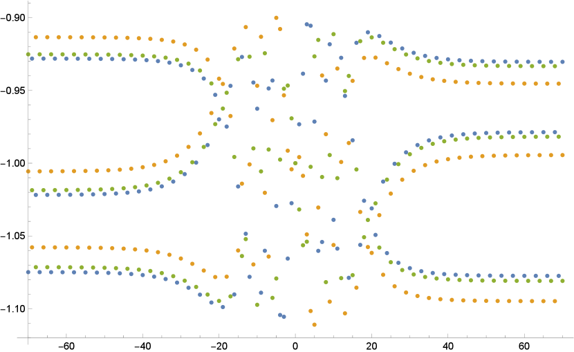
$q\textrm{P}_{\textrm{IV}}(a)|_{t_{0}=i}$ has precisely four symmetric solutions, which are all regular at $t=i$ , each specified by its initial values at $m=0$ , with the four possible initial conditions given by

(f_{0}(i),f_{1}(i),f_{2}(i))=\begin{cases}(-1,1,1),\\ (1,-1,1),\\ (1,1,-1),\\ (-1,-1,-1).\end{cases}

See Figure 1 for a plot of one the symmetric solutions.

Refer to caption — Figure 1. Numerical display of the symmetric solution in Lemma 2.2 with initial conditions $(f_{0}(i),f_{1}(i),f_{2}(i))=(-1,-1,-1)$ . The values of $q^{-\frac{2}{3}m}f_{k}(q^{m}i)$ , $k=0,1,2$ , are displayed in respectively blue, orange and green, with $m$ ranging from -70 to 70 on the horizontal axis. The values of the parameters are $a_{0}=q^{\frac{9}{23}}$ , $a_{1}=q^{\frac{8}{23}}$ and $a_{2}=q^{\frac{6}{23}}$ , with $q=0.802$ .

Remark 2.3.

It is instructive to compare this with the symmetric solutions of $S\textrm{P}_{\textrm{IV}}(\alpha)$ . In accordance with the definition of symmetric solutions of $\textrm{P}_{\textrm{IV}}$ , see Kaneko [kaneko2005], these are solutions $g$ of $S\textrm{P}_{\textrm{IV}}(\alpha)$ that satisfy

g_{k}(s)=-g_{k}(-s)\quad(k=0,1,2).

$S\textrm{P}_{\textrm{IV}}(\alpha)$ has precisely four symmetric solutions. Three non-analytic at $s=0$ , with Laurent series in a domain around $s=0$ given by

{\rm Case\ I:}\quad\begin{cases}g_{0}(s)&=-\alpha_{0}s+\mathcal{O}\left(s^{3}\right),\\ g_{1}(s)&=+s^{-1}+\mathcal{O}\left(s\right),\\ g_{2}(s)&=-s^{-1}+\mathcal{O}\left(s\right),\end{cases}

{\rm Case\ II:}\quad\begin{cases}g_{0}(s)&=-s^{-1}+\mathcal{O}\left(s\right),\\ g_{1}(s)&=-\alpha_{1}s+\mathcal{O}\left(s^{3}\right),\\ g_{2}(s)&=+s^{-1}+\mathcal{O}\left(s\right),\end{cases}

{\rm Case\ III:}\quad\begin{cases}g_{0}(s)&=+s^{-1}+\mathcal{O}\left(s\right),\\ g_{1}(s)&=-s^{-1}+\mathcal{O}\left(s\right),\\ g_{2}(s)&=-\alpha_{2}s+\mathcal{O}\left(s^{3}\right),\end{cases}

and one analytic at $s=0$ , specified by

{\rm Case\ IV:}\quad g_{k}(s)=\alpha_{k}s+\mathcal{O}\left(s^{3}\right)\quad(s\rightarrow 0),

for $k=0,1,2$ .

3. Symmetries and the linear problem

In this section, we recall some essential aspects of the linear problem associated with $q\textrm{P}_{\textrm{IV}}$ and study their interplay with the symmetries $\mathcal{T}_{\pm}$ .

In Section 3.1 we recall the Lax pair associated with $q\textrm{P}_{\textrm{IV}}$ and lift the action of $\mathcal{T}_{\pm}$ to it. Then, in Section 3.15, we introduce the connection matrix associated with the linear problem and derive how the symmetries act on it. Finally, in Section 3.3, we compute how $\mathcal{T}_{\pm}$ transform certain monodromy coordinates and provide an alternative way to classify symmetric solutions.

3.1. The Lax pair

We recall the following Lax pair of $q\textrm{P}_{\textrm{IV}}$ , derived in [joshinobu2016],


$\displaystyle Y(qz,t)$	$\displaystyle=A(z,t)Y(z,t),$	(3.1a)
$\displaystyle Y(z,qt)$	$\displaystyle=B(z,t)Y(z,t),$	(3.1b)

where


$\displaystyle A:=$	$\displaystyle\begin{pmatrix}u&0\\ 0&1\end{pmatrix}\begin{pmatrix}-i\,q\frac{t}{f_{2}}z&1\\ -1&-\,i\,q\frac{f_{2}}{t}z\end{pmatrix}\begin{pmatrix}-\,i\,a_{0}a_{2}\frac{t}{f_{0}}z&1\\ -1&-\,i\,a_{0}a_{2}\frac{f_{0}}{t}z\end{pmatrix}\times$
	$\displaystyle\ \times\,\begin{pmatrix}-\,i\,a_{0}\frac{t}{f_{1}}z&1\\ -1&-\,i\,a_{0}\frac{f_{1}}{t}z\end{pmatrix}\begin{pmatrix}u^{-1}&0\\ 0&1\end{pmatrix},$	(3.2a)
$\displaystyle B:=$	$\displaystyle\begin{pmatrix}0&-bu\\ b^{-1}u^{-1}&0\end{pmatrix}+\begin{pmatrix}z&0\\ 0&0\end{pmatrix}\,,$	(3.2b)

with

b=\frac{t(1+a_{1}f_{1}(1+a_{2}f_{2}))}{i\,(qt^{2}-1)f_{2}}.

(3.3)

We refer to the first equation of the Lax pair, equation (3.1a), as the spectral equation.

Compatibility of the Lax pair,

A(z,qt)B(z,t)=B(qz,t)A(z,t),

(3.4)

is equivalent to $(f_{0},f_{1},f_{2})$ satisfying $q\textrm{P}_{\textrm{IV}}(a)$ and $u$ satisfying the auxiliary equation

\frac{\overline{u}}{u}=b^{2}.

(3.5)

We proceed to lift the symmetries $\mathcal{T}_{\pm}$ to this Lax pair. To this end, the following notation will be helpful. For any $2\times 2$ matrix $U$ , we let $U^{\diamond}$ denotes the co-factor matrix, or adjugate transpose, of $U$ . In other words,

\begin{pmatrix}a&b\\ c&d\end{pmatrix}^{\diamond}=\begin{pmatrix}d&-c\\ -b&a\end{pmatrix}.

We further remind the reader that some of the notation used in this paper, is outlined in Appendix A.

Lemma 3.1.

The symmetry $\mathcal{T}_{+}$ extends to the following symmetry of the Lax pair,

	$\displaystyle Y(z,t)$	$\displaystyle\mapsto\widetilde{Y}(z,t)=Y^{\diamond}(z,1/t),$
	$\displaystyle A(z,t)$	$\displaystyle\mapsto\widetilde{A}(z,t)=A^{\diamond}(z,1/t),$
	$\displaystyle B(z,t)$	$\displaystyle\mapsto\widetilde{B}(z,t)=B^{T}(z,1/(qt)),$

and, consequently,

u(t)\mapsto\widetilde{u}(t)=\frac{1}{u(1/t)},\quad b(t)\mapsto\widetilde{b}(t)=-b(1/(qt)).

Similarly, the symmetry $\mathcal{T}_{-}$ extends to the following symmetry of the Lax pair,

	$\displaystyle Y(z,t)$	$\displaystyle\mapsto\widetilde{Y}(z,t)=r(z)\sigma_{3}Y^{\diamond}(z,-1/t),$
	$\displaystyle A(z,t)$	$\displaystyle\mapsto\widetilde{A}(z,t)=-\sigma_{3}A^{\diamond}(z,-1/t)\sigma_{3},$
	$\displaystyle B(z,t)$	$\displaystyle\mapsto\widetilde{B}(z,t)=\sigma_{3}B^{T}(z,-1/(qt))\sigma_{3},$

where $r(z)$ any function that satisfies $r(qz)=-r(z)$ , and, consequently,

u\mapsto\widetilde{u}(t)=\frac{1}{u(-1/t)},\quad b(t)\mapsto\widetilde{b}(t)=b(-1/(qt)).

Proof.

We only prove the extension of the first symmetry. The other one follows analogously.

Let us denote $A(z,t)=\mathcal{A}(z,t,f_{0},f_{1},f_{2},u)$ and $B(z,t)=\mathcal{B}(z,t,b,u)$ and consider the transformation

\mathcal{T}:Y(z,t)\mapsto\widetilde{Y}(z,t)=Y^{\diamond}(z,1/t).

This transformation induces the following action on the Lax matrices,

	$\displaystyle A(z,t)$	$\displaystyle\mapsto\widetilde{A}(z,t)=A^{\diamond}(z,1/t),$
	$\displaystyle B(z,t)$	$\displaystyle\mapsto\widetilde{B}(z,t)=B^{T}(z,1/(qt)).$

As $(UV)^{\diamond}=U^{\diamond}V^{\diamond}$ , it follows that

	$\displaystyle A^{\diamond}(z,1/t)$	$\displaystyle=\mathcal{A}^{\diamond}(z,1/t,f_{0}(1/t),f_{1}(1/t),f_{2}(1/t),u(1/t))$
		$\displaystyle=\mathcal{A}(z,t,F_{0}(t),F_{1}(t),F_{2}(t),\widetilde{u}(t)),$

with

\widetilde{u}(t)=\frac{1}{u(1/t)},\quad F_{k}(t)=\frac{1}{f_{k}(1/t)}\quad(k=0,1,2).

Note that this is consistent with the symmetry $\mathcal{T}_{+}$ , so that $\mathcal{T}$ indeed defines an extension of $\mathcal{T}_{+}$ .

It remains to be checked that the action of $\mathcal{T}$ of $B(z,t)$ is consistent with its action on $A(z,t)$ . That is, we need to ensure that

\mathcal{B}^{T}(z,1/(qt),b(1/(qt)),u(1/(qt)))=\mathcal{B}(z,t,\widetilde{b}(t),\widetilde{u}(t)),

(3.6)

where, in acccordance with equation (3.3),

\widetilde{b}(t)=\frac{t(1+a_{1}F_{1}(t)(1+a_{2}F_{2}(t))}{i\,(qt^{2}-1)F_{2}(t)}.

Now, equation (3.6) holds if and only if

\widetilde{b}(t)\widetilde{u}(t)=-\frac{1}{b(1/(qt)),u(1/(qt))}.

By substituting the expression for $\widetilde{u}(t)$ , it follows that this is equivalent to

\widetilde{b}(t)=-\frac{u(1/t)}{b(1/(qt)),u(1/(qt))}.

By the auxiliary equation (3.5), we have $b^{2}=\overline{u}/u$ , which simplifies the right-hand side, so that the identify to prove simply reads

\widetilde{b}(t)=-b(1/(qt)).

The last equality follows by direct computation, using the $q\textrm{P}_{\textrm{IV}}$ time-evolution equations.

Finally, we note that the transformation $\mathcal{T}$ preserves the compatibility condition of the Lax pair (3.4), which reaffirms the fact that $(F_{0},F_{1},F_{2})$ is another solution of $q\textrm{P}_{\textrm{IV}}$ , and further shows that $\widetilde{u}$ solves the corresponding auxiliary equation. ∎

Now, consider any symmetric solution of $q\textrm{P}_{\textrm{IV}}$ with respect to $\mathcal{T}_{-}$ , then we can choose a corresponding solution $u$ of the auxiliary equation such that the Lax matrices have the symmetries

	$\displaystyle A(z,t)$	$\displaystyle=-\sigma_{3}A^{\diamond}(z,-1/t)\sigma_{3},$
	$\displaystyle B(z,t)$	$\displaystyle=\sigma_{3}B^{T}(z,-1/(qt))\sigma_{3}.$

By specialising the first equation to $t=i$ , we then find

A(z,i)=-\sigma_{3}A^{\diamond}(z,i)\sigma_{3}.

(3.7)

This provides another way to classify the symmetric solutions of $q\textrm{P}_{\textrm{IV}}(a)|_{t_{0}=i}$ , by computing all the coefficient matrices $A(z,i)$ that possess the symmetry (3.7).

3.2. The connection matrix

In this section, we introduce the connection matrix associated with the Lax pair and deduce how the symmetries $\mathcal{T}_{\pm}$ act on it.

Firstly, we introduce a canonical solution at $z=\infty$ in the following lemma.

Lemma 3.2.

[Lemma 3.3 in [joshiroffelsenrhp]] For any fixed $t$ , there exists a unique $2\times 2$ matrix $\Phi_{\infty}(z,t)$ , meromorphic in $z$ on $\mathbb{C}^{*}$ , such that

	$\displaystyle\Phi_{\infty}(qz,t)$	$\displaystyle=\frac{1}{qa_{0}^{2}a_{2}i}z^{-3}A(z,t)\Phi_{\infty}(z,t)\begin{pmatrix}t^{-1}&0\\ 0&t\end{pmatrix},$		(3.8)
	$\displaystyle\Phi_{\infty}(z,t)$	$\displaystyle=I+\mathcal{O}\left(z^{-1}\right)\quad(z\rightarrow\infty).$		(3.9)

In particular,

Y_{\infty}(z,t)=\Phi_{\infty}(z,t)\begin{pmatrix}r_{+}(z,t)&0\\ 0&r_{-}(z,t)\end{pmatrix}

defines a solution of the spectral equation (3.1a), for any choice of functions $r_{\pm}(z,t)$ satisfying

\frac{r_{\pm}(qz,t)}{r_{\pm}(z,t)}=qa_{0}^{2}a_{2}iz^{-3}t^{\pm 1}.

Lemma 3.3.

[Lemma 3.2 in [joshiroffelsenrhp]] For any fixed $t$ and $d\in\mathbb{C}^{*}$ , we have

A(0)=M_{0}\begin{pmatrix}i&0\\ 0&-i\end{pmatrix}M_{0}^{-1},\textrm{ where }M_{0}:=d\begin{pmatrix}u&0\\ 0&1\end{pmatrix}\cdot\begin{pmatrix}i&-i\\ 1&1\end{pmatrix},

(3.10)

and, there exists a unique $2\times 2$ matrix $\Phi_{0}(z,t)$ , meromorphic in $z$ on $\mathbb{C}^{*}$ , such that

	$\displaystyle\Phi_{0}(qz,t)$	$\displaystyle=A(z,t)\Phi_{0}(z,t)\begin{pmatrix}-i&0\\ 0&i\end{pmatrix},$		(3.11)
	$\displaystyle\Phi_{0}(z,t)$	$\displaystyle=M_{0}+\mathcal{O}\left(z\right),\ {\rm as}\ z\rightarrow 0.$

In particular, it follows that

Y_{0}(z,t)=\Phi_{0}(z,t)r_{0}(z)^{\sigma_{3}},

defines a solution of the spectral equation (3.1a), for any choice of meromorphic function $r_{0}(z)$ satisfying $r_{0}(qz)=i\,r_{0}(z)$ .

We define the corresponding connection matrix by

C(z,t)=\Phi_{0}(z,t)^{-1}\Phi_{\infty}(z,t),

(3.12)

which satisfies, see [joshiroffelsenrhp], for fixed $t$ ,

(c.1)

$C(z,t)$ is analytic in $z$ on $\mathbb{C}^{*}$ ;
(c.2)

$C(qz,t)=\frac{1}{qa_{0}^{2}a_{2}}z^{-3}\sigma_{3}C(z,t)t^{-\sigma_{3}}$ ;
(c.3)

$|C(z,t)|=c\,\theta_{q}(a_{0}z,-a_{0}z,a_{0}a_{2}z,-a_{0}a_{2}z,qz,-qz)$ , for some $c\neq 0$ ;
(c.4)

$C(-z,t)=-\sigma_{1}C(z,t)\sigma_{3}$ .

It follows from the compatibility condition (3.4), see [joshiroffelsenrhp] for more details, that

	$\displaystyle\Phi_{\infty}(z,qt)$	$\displaystyle=B(z,t)\Phi_{\infty}(z,t)z^{-\sigma_{3}},$
	$\displaystyle\Phi_{0}(z,qt)$	$\displaystyle=B(z,t)\Phi_{0}(z,t)\sigma_{3},$

which yields the almost trivial time-evolution of the connection matrix,

C(z,qt)=\sigma_{3}C(z,t)z^{-\sigma_{3}},

(3.13)

as well as the time-evolution of $d$ in Lemma 3.3,

\frac{\overline{d}}{d}=\frac{i}{b}.

(3.14)

The connection matrix encompasses the monodromy of the Lax pair. In particular, one can in principle uniquely reconstruct the linear system (3.1a) from the connection matrix by solving an associated Riemann-Hilbert problem.

We will now extend the action of the symmetries to the connection matrix.

Lemma 3.4.

The transformation $\mathcal{T}_{+}$ extends to the following symmetry of the canonical solutions and connection matrix,

	$\displaystyle\Phi_{\infty}(z,t)$	$\displaystyle\mapsto\widetilde{\Phi}_{\infty}(z,t)=\Phi_{\infty}^{\diamond}(z,1/t),$
	$\displaystyle\Phi_{0}(z,t)$	$\displaystyle\mapsto\widetilde{\Phi}_{0}(z,t)=-i\,\Phi_{0}^{\diamond}(z,1/t)\sigma_{1},$
	$\displaystyle C(z,t)$	$\displaystyle\mapsto\widetilde{C}(z,t)=i\,\sigma_{1}C^{\diamond}(z,1/t).$

The transformation $\mathcal{T}_{-}$ extends to the following symmetry of the canonical solutions and connection matrix,

	$\displaystyle\Phi_{\infty}(z,t)$	$\displaystyle\mapsto\widetilde{\Phi}_{\infty}(z,t)=\sigma_{3}\Phi_{\infty}^{\diamond}(z,-1/t)\sigma_{3},$
	$\displaystyle\Phi_{0}(z,t)$	$\displaystyle\mapsto\widetilde{\Phi}_{0}(z,t)=i\,\sigma_{3}\Phi_{0}^{\diamond}(z,-1/t),$
	$\displaystyle C(z,t)$	$\displaystyle\mapsto\widetilde{C}(z,t)=-i\,C^{\diamond}(z,1/t)\sigma_{3}.$

Furthermore, $\mathcal{T}_{\pm}$ act on $d$ , defined in Lemma 3.3, by

d(t)\mapsto\widetilde{d}(t)=d(\pm 1/t)u(\pm 1/t).

Proof.

We only prove the extension for $\mathcal{T}_{-}$ . The extension of $\mathcal{T}_{+}$ is proven analogously.

We first consider the canonical solution at $z=\infty$ . In fact, by Lemma 3.2, the matrix function $\Phi_{\infty}(z,t)$ is defined uniquely as the solution to (3.8) and (3.9). This means that the action of $\mathcal{T}_{-}$ on $\Phi_{\infty}(z,t)$ is already fixed by its action on the Lax matrix $A(z,t)$ .

To determine it explicitly, we first apply $t\mapsto-1/t$ to equation (3.8), which yields

\Phi_{\infty}(qz,-1/t)=-\frac{1}{qa_{0}^{2}a_{2}i}z^{-3}A(z,-1/t)\Phi_{\infty}(z,-1/t)\begin{pmatrix}t&0\\ 0&t^{-1}\end{pmatrix}.

Next, applying $U\mapsto U^{\diamond}$ to both sides, we obtain

\Phi_{\infty}^{\diamond}(qz,-1/t)=-\frac{1}{qa_{0}^{2}a_{2}i}z^{-3}A^{\diamond}(z,-1/t)\Phi_{\infty}^{\diamond}(z,t)\begin{pmatrix}t^{-1}&0\\ 0&t\end{pmatrix}.

Finally, multiplying both sides from the left and right by $\sigma_{3}$ , we obtain

\widetilde{\Phi}_{\infty}(qz,t)=\frac{1}{qa_{0}^{2}a_{2}i}z^{-3}\widetilde{A}(z,t)\widetilde{\Phi}_{\infty}(z,t)\begin{pmatrix}t^{-1}&0\\ 0&t\end{pmatrix},

with

\widetilde{A}(z,t)=-\sigma_{3}A^{\diamond}(z,-1/t)\sigma_{3},\qquad\widetilde{\Phi}_{\infty}(z,t)=\sigma_{3}\Phi_{\infty}^{\diamond}(z,-1/t)\sigma_{3}.

Note that, furthermore, the normalisation at $z=\infty$ is correct, namely $\widetilde{\Phi}_{\infty}(z,t)=I+\mathcal{O}(z^{-1})$ as $z\rightarrow\infty$ . We conclude, from Lemma 3.2, that $\mathcal{T}_{-}$ indeed sends $\Phi_{\infty}(z,t)$ to $\widetilde{\Phi}_{\infty}(z,t)$ .

We next consider the canonical solution at $z=0$ . The matrix function $\Phi_{0}(z)$ , see Lemma 3.3, is only rigidly defined up to the choice of a scalar $d=d(t)$ which satisfies $\overline{d}/d=i/b$ , see equation (3.14). So, in order to fix the action of the symmetry $\mathcal{T}_{-}$ on $\Phi_{0}(z)$ , we first need to fix its action on $d$ in such a way that $\overline{d}/d=i/b$ remains to hold true. Namely, it is required that, if we let $d\mapsto\widetilde{d}$ under $\mathcal{T}_{-}$ , then

\frac{\widetilde{d}(qt)}{\widetilde{d}(t)}=\frac{i}{\widetilde{b}(t)}=-\frac{i}{b(-1/(qt))}.

We therefore set $\widetilde{d}(t)=d(-1/t)u(-1/t)$ , so that indeed

\frac{\widetilde{d}(qt)}{\widetilde{d}(t)}=\frac{d(-1/(qt))}{d(-1/t)}\frac{u(-1/(qt))}{u(-1/t)}=\frac{b(-1/(qt))}{i}\frac{1}{b(-1/(qt))^{2}}=-\frac{i}{b(-1/(qt))}.

By essentially repeating the computation for $\Phi_{\infty}(z)$ above, for $\Phi_{0}(z)$ , one finds that

\widetilde{\Phi}_{0}(z,t)=i\,\sigma_{3}\Phi_{0}^{\diamond}(z,-1/t),

defines a solution to, see equation (3.11),

\widetilde{\Phi}_{0}(qz,t)=\widetilde{A}(z,t)\widetilde{\Phi}_{0}(z,t)\begin{pmatrix}-i&0\\ 0&i\end{pmatrix}.

Furthermore, direct evaluation of $\widetilde{\Phi}_{0}(z,t)$ at $z=0$ gives

	$\displaystyle\widetilde{\Phi}_{0}(0,t)$	$\displaystyle=i\,\sigma_{3}\Phi_{0}^{\diamond}(0,-1/t),$
		$\displaystyle=i\,d(-1/t)\sigma_{3}\begin{pmatrix}1&0\\ 0&u(-1/t)\end{pmatrix}\cdot\begin{pmatrix}1&-1\\ i&i\end{pmatrix},$
		$\displaystyle=d(-1/t)\begin{pmatrix}1&0\\ 0&u(-1/t)\end{pmatrix}\cdot\begin{pmatrix}i&-i\\ 1&1\end{pmatrix}$
		$\displaystyle=\widetilde{d}(t)\begin{pmatrix}\widetilde{u}(t)&0\\ 0&1\end{pmatrix}\cdot\begin{pmatrix}i&-i\\ 1&1\end{pmatrix}.$

It follows that $\mathcal{T}_{-}$ sends $\Phi_{0}(z,t)$ to $\widetilde{\Phi}_{0}(z,t)$ .

Finally, we compute the action of $\mathcal{T}_{-}$ on the connection matrix. Since $U\mapsto U^{\diamond}$ commutes with inversion, $U\mapsto U^{-1}$ , we have

	$\displaystyle\widetilde{C}(z,t)$	$\displaystyle=\widetilde{\Phi}_{0}(z,t)^{-1}\widetilde{\Phi}_{\infty}(z,t)$
		$\displaystyle=\left[i\,\sigma_{3}\Phi_{0}^{\diamond}(z,-1/t)\right]^{-1}\sigma_{3}\Phi_{\infty}^{\diamond}(z,-1/t)\sigma_{3}$
		$\displaystyle=-i\left[\Phi_{0}^{\diamond}(z,-1/t)\right]^{-1}\Phi_{\infty}^{\diamond}(z,-1/t)\sigma_{3}$
		$\displaystyle=-i\,C^{\diamond}(z,-1/t)\sigma_{3}.$

This finishes the proof of the lemma. ∎

Now, let us take any symmetric solution of $q\textrm{P}_{\textrm{IV}}$ with respect to $\mathcal{T}_{-}$ , then we can choose a corresponding solution $u$ of the auxiliary equation, as well as $d$ satisfying (3.14), such that the connection matrix has the symmetry

C(z,t)=-i\,C^{\diamond}(z,-1/t)\sigma_{3}.

By specialising this equation to $t=i$ , we then find

C(z,i)=-i\,C^{\diamond}(z,i)\sigma_{3}.

(3.15)

This provides yet a third way to classify symmetric solutions of $q\textrm{P}_{\textrm{IV}}(a)|_{t_{0}=i}$ , by classifying all connection matrices $C(z,i)$ with the symmetry (3.15).

3.3. Monodromy coordinates

In [joshiroffelsenrhp], we introduced a set of coordinates on the connection matrix, which are invariant under right-multiplication of the connection matrix by diagonal matrices. They are given by

\rho_{k}(t)=\pi(C(x_{k},t)),\quad(1\leq k\leq 3),\quad(x_{1},x_{2},x_{3})=(a_{0}^{-1},a_{1}/q,q^{-1}),

where, for any rank one $2\times 2$ matrix $R$ , letting $r_{1}$ and $r_{2}$ be respectively its first and second row, $\pi(R)\in\mathbb{CP}^{1}$ is defined by

r_{1}=\pi(R)r_{2}.

This yields three coordinates, $\rho=(\rho_{1},\rho_{2},\rho_{3})\in(\mathbb{CP}^{1})^{3}$ , which satisfy the cubic equation,

$\displaystyle 0=$	$\displaystyle+\beta_{0}\left[\theta_{q}(t)\rho_{1}\rho_{2}\rho_{3}-\theta_{q}(-t)\right]$	(3.16)
	$\displaystyle-\beta_{1}\left[\theta_{q}(t)\rho_{1}-\theta_{q}(-t)\rho_{2}\rho_{3}\right]$
	$\displaystyle+\beta_{2}\left[\theta_{q}(t)\rho_{2}-\theta_{q}(-t)\rho_{1}\rho_{3}\right]$
	$\displaystyle-\beta_{3}\left[\theta_{q}(t)\rho_{3}-\theta_{q}(-t)\rho_{1}\rho_{2}\right].$

with coefficients given by

	$\displaystyle\beta_{0}$	$\displaystyle=\theta_{q}(+a_{0},+a_{1},+a_{2}),$
	$\displaystyle\beta_{1}$	$\displaystyle=\theta_{q}(-a_{0},+a_{1},-a_{2}),$
	$\displaystyle\beta_{2}$	$\displaystyle=\theta_{q}(+a_{0},-a_{1},-a_{2}),$
	$\displaystyle\beta_{3}$	$\displaystyle=\theta_{q}(-a_{0},-a_{1},+a_{2}).$

When considering solutions defined on a discrete $q$ -spiral, i.e. $t\in q^{\mathbb{Z}}t_{0}$ , the value of $p:=\rho(t_{0})$ uniquely determines the corresponding solution $(f_{0},f_{1},f_{2})$ of $q\textrm{P}_{\textrm{IV}}(a)$ [joshiroffelsenrhp].

In the following proposition, the action of the symmetries on the monodromy coordinates is determined.

Proposition 3.5.

The symmetry $\mathcal{T}_{+}$ acts on the monodromy coordinates by

\rho_{k}(t)\mapsto\widetilde{\rho}_{k}(t)=-\rho_{k}(1/t)\quad(k=1,2,3).

The symmetry $\mathcal{T}_{-}$ acts on the monodromy coordinates by

\rho_{k}(t)\mapsto\widetilde{\rho}_{k}(t)=-\frac{1}{\rho_{k}(-1/t)}\quad(k=1,2,3).

Proof.

To compute the action of the symmetries on the monodromy coordinates, we need some basic facts about the operator $\pi(\cdot)$ . Firstly, given any rank one $2\times 2$ matrix $R$ , and invertible $2\times 2$ matrix $N=(n_{ij})$ , we have

\pi(RN)=\pi(R),\quad\pi(NR)=\chi_{N}(\pi(R)),

(3.17)

where $\chi_{N}$ denotes the möbius transformation

\chi_{N}(z)=\frac{n_{11}z+n_{12}}{n_{21}z+n_{22}}.

In particular,

\pi(\sigma_{1}R)=\chi_{\sigma_{1}}(\pi(R))=1/\pi(R).

Secondly, it is elementary to check that

\pi(R^{\diamond})=-1/\pi(R).

We now compute, for transformation $\mathcal{T}_{+}$ ,

	$\displaystyle\widetilde{\rho}_{k}(t)$	$\displaystyle=\pi[\widetilde{C}(x_{k},t)]=\pi[i\,\sigma_{1}C^{\diamond}(x_{k},1/t)]=\pi[\sigma_{1}C^{\diamond}(x_{k},1/t)]$
		$\displaystyle=1/\pi[C^{\diamond}(x_{k},1/t)]=-\pi[C(x_{k},1/t)]=-\rho_{k}(1/t).$

Similarly, for transformation $\mathcal{T}_{-}$ , we have

	$\displaystyle\widetilde{\rho}_{k}(t)$	$\displaystyle=\pi[\widetilde{C}(x_{k},t)]=\pi[-i\,C^{\diamond}(x_{k},-1/t)\sigma_{3}]=\pi[C^{\diamond}(x_{k},-1/t)]$
		$\displaystyle=-\frac{1}{\pi[C(x_{k},-1/t)]}=-\frac{1}{\rho_{k}(-1/t)},$

and the proposition follows. ∎

In the sequel, the following technical lemma will be of importance. Its proof is given in Appendix B.

Lemma 3.6.

Let $t_{0}$ , with $t_{0}^{2}\notin q^{\mathbb{Z}}$ , be inside the domain of a solution $f=(f_{0},f_{1},f_{2})$ of $q\textrm{P}_{\textrm{IV}}$ . If $f(t)$ takes at least one non-singular value, i.e. a value in $(\mathbb{C}^{*})^{3}$ , at a point $t\in q^{\mathbb{Z}}t_{0}$ , then the coordinates $p=\rho(t_{0})$ cannot lie on the curve defined by the intersection of the following equations in $(\mathbb{CP}^{1})^{3}$ ,

	$\displaystyle 0=$	$\displaystyle+\beta_{0}p_{1}p_{2}p_{3}-\beta_{1}p_{1}+\beta_{2}p_{2}-\beta_{3}p_{3},$		(3.18)
	$\displaystyle 0=$	$\displaystyle+\beta_{0}-\beta_{1}p_{2}p_{3}+\beta_{2}p_{1}p_{3}-\beta_{3}p_{1}p_{2},$

with the same coefficients as the cubic (3.16). We note that points on this curve solve the cubic equation (3.16) irrespective of the value of $t$ .

Let us now take any solution $f$ of $q\textrm{P}_{\textrm{IV}}(a)|_{t_{0}=i}$ on the $q$ -spiral $q^{\mathbb{Z}}i$ . To it, corresponds a unique triplet $p=(p_{1},p_{2},p_{3})$ , defined by $p_{k}:=\rho_{k}(i)$ , $k=1,2,3$ , which satisfies the cubic equation

	$\displaystyle 0=$	$\displaystyle+\theta_{q}(+a_{0},+a_{1},+a_{2})\left(p_{1}p_{2}p_{3}-i\right)$
		$\displaystyle-\theta_{q}(-a_{0},+a_{1},-a_{2})\left(p_{1}-i\,p_{2}p_{3}\right)$
		$\displaystyle+\theta_{q}(+a_{0},-a_{1},-a_{2})\left(p_{2}-i\,p_{1}p_{3}\right)$
		$\displaystyle-\theta_{q}(-a_{0},-a_{1},+a_{2})\left(p_{3}-i\,p_{1}p_{2}\right),$

as follows from the identity $\theta_{q}(-i)=i\,\theta_{q}(i)$ , and does not lie on the curve defined by by equations (3.18).

Note that $\widetilde{f}=\mathcal{T}_{-}(f)$ defines another solution on the same domain $q^{\mathbb{Z}}i$ , and its monodromy coordinates, $\widetilde{p}_{k}:=\widetilde{\rho}_{k}(i)$ , $k=1,2,3$ , are related to those of $f$ by

\widetilde{p}_{k}=-1/p_{k}\quad(k=1,2,3).

In particular, $f$ is a symmetric solution if and only if $\widetilde{f}=f$ , which in turn is equivalent to

p_{k}=-1/p_{k}\quad(k=1,2,3).

(3.19)

In other words, symmetric solutions of $q\textrm{P}_{\textrm{IV}}(a)|_{t_{0}=i}$ correspond to monodromy coordinates $p$ which satisfy the cubic equation above as well as (3.19).

We proceed to compute four triples $p$ that satisfy these conditions. Firstly, equation (3.19) has only two solutions in $\mathbb{CP}^{1}$ , given by $\pm i$ , and we may thus set $p_{k}=\epsilon_{k}i$ , $\epsilon_{k}=\pm 1$ , $k=1,2,3$ . Substitution of these into the cubic shows that the latter is identically zero if the epsilons satisfy

\epsilon_{1}\epsilon_{2}\epsilon_{3}=-1,

as in such a case

p_{1}p_{2}p_{3}-i=p_{j}-i\,p_{k}p_{l}=0\qquad(\{j,k,l\}=\{1,2,3\}).

In particular, this gives us four solutions,

(p_{1},p_{2},p_{3})\in\{(-i,-i,-i),(-i,i,i),(i,-i,i),(i,i,-i)\},

(3.20)

corresponding to the four symmetric solutions in Lemma 2.2.

Whilst for generic values of the parameters, these are the only solutions to the cubic, it may so happen for special values of the parameters, that there is a choice of epsilons, with

\epsilon_{1}\epsilon_{2}\epsilon_{3}=+1,

that also solves the cubic. But in such a case, a direct computation yields

-\beta_{0}-\beta_{1}\epsilon_{1}+\beta_{2}\epsilon_{2}-\beta_{3}\epsilon_{3}=0,

and thus the point $(p_{1},p_{2},p_{3})$ lies on the curve (3.18) and hence does not correspond to a solution of $q\textrm{P}_{\textrm{IV}}$ .

In the next section, Section 4, we derive which values of the coordinates in equation (3.20) correspond to which initial conditions

(f_{0}(i),f_{1}(i),f_{2}(i))\in\{(-1,-1,-1),(-1,1,1),(1,-1,1),(1,1,-1)\}.

We answer this question by explicitly solving the linear problem at the reflection point $t=i$ for each case; see Theorem 4.1.

4. Explicit solvability of the linear problem at a reflection point

In this section we show that the linear problem is explicitly solvable at the reflection point $t_{0}=i$ , for symmetric solutions. In particular, we will prove the following theorem in the end of Section 4.2.

Theorem 4.1.

Let $(f_{0},f_{1},f_{2})$ be a symmetric solution of $q\textrm{P}_{\textrm{IV}}(a)|_{t_{0}=i}$ , invariant under $\mathcal{T}_{-}$ , satisfying initial conditions

(f_{0}(i),f_{1}(i),f_{2}(i))=(v_{0},v_{1},v_{2}),

so that (by Lemma 2.2),

(v_{0},v_{1},v_{2})\in\{(-1,-1,-1),(-1,1,1),(1,-1,1),(1,1,-1)\}.

Fix the auxiliary functions $u$ and $d$ by the initial conditions $u(i)=1$ and $d(i)=i$ . Then, the connection matrix at $t=i$ is explicitly given by

C(z,i)=2c_{0}^{3}\begin{pmatrix}h(i\,z)&i\,h(-i\,z)\\ -h(-i\,z)&i\,h(i\,z)\end{pmatrix},

(4.1)

where the scalar $c_{0}$ equals

c_{0}=\frac{\sqrt{i}\,\theta_{q}(i)}{\sqrt{2}\,\theta_{q}(-1)}=\frac{1}{2}\prod_{k=1}^{\infty}{\frac{(1+q^{k}i)(1-q^{k}i)}{(1+q^{k})^{2}}},

and the function $h(z)$ is defined by

	$\displaystyle h(z)=$	$\displaystyle+\theta_{q}\bigg{(}+\frac{v_{1}}{x_{1}}z,-\frac{v_{0}}{x_{2}}z,+\frac{v_{2}}{x_{3}}z\bigg{)}-\theta_{q}\bigg{(}+\frac{v_{1}}{x_{1}}z,+\frac{v_{0}}{x_{2}}z,-\frac{v_{2}}{x_{3}}z\bigg{)}$
		$\displaystyle-\theta_{q}\bigg{(}-\frac{v_{1}}{x_{1}}z,-\frac{v_{0}}{x_{2}}z,-\frac{v_{2}}{x_{3}}z\bigg{)}-\theta_{q}\bigg{(}-\frac{v_{1}}{x_{1}}z,+\frac{v_{0}}{x_{2}}z,+\frac{v_{2}}{x_{3}}z\bigg{)},$

with

(x_{1},x_{2},x_{3})=(a_{0}^{-1},a_{1}/q,q^{-1}).

In particular, the corresponding values of the monodromy coordinates, $p_{k}=\rho_{k}(i)$ , $k=1,2,3$ , are given by

(p_{1},p_{2},p_{3})=(-v_{1}i,v_{0}i,-v_{2}i).

(4.2)

Remark 4.2.

In the proof of Theorem 4.1, we also obtain the following alternative expression for the connection matrix,

C(z)=\sigma_{1}C_{0}\left(\frac{v_{1}}{x_{1}}z\right)MC_{0}\left(-\frac{v_{0}}{x_{2}}z\right)MC_{0}\left(\frac{v_{2}}{x_{3}}z\right),

where $C_{0}(z)$ , given in Proposition 4.5, is the connection matrix of a degree one Fuchsian system and the matrix $M$ is defined in equation (4.6).

The spectral equation of the Lax pair (1.3) naturally comes in a factorised form. The fundamental reason that allows us to solve the linear problem at the reflection point $t=i$ , for a symmetric solution as in Theorem 4.1, is that the factors in this form ‘almost’ commute. Namely, by fixing $u(i)=1$ , we have

A(z,i)=A_{0}\left(\frac{v_{2}z}{x_{3}}\right)A_{0}\left(\frac{v_{0}z}{x_{2}}\right)A_{0}\left(\frac{v_{1}z}{x_{1}}\right),

where

A_{0}(z)=i\,\sigma_{2}+z\,\sigma_{3},

and these factors satisfy the commutation relation,

A_{0}(x)A_{0}(y)=A_{0}(-y)A_{0}(-x).

(4.3)

This observation allows us to construct global solutions of the linear system

Y(qz)=A(z,i)Y(z),

from solutions of the simpler system

U(qz)=A_{0}(z)U(z),

which we will refer to as the model problem.

In Section 4.1, we solve this model problem, and in Section 4.2 we use this to construct global solutions of the spectral equation at $t=i$ and prove Theorem 4.1. The model problem is solved in terms of basic hypergeometric functions, denoted for given parameter $a$ , $0<p<1$ and $z\in\mathbb{C}$ by

{}_{0}\phi_{1}\left[\begin{matrix}\text{-}\\ a\end{matrix};p,z\right],

whose mathematical properties can be found in [gasper].

4.1. The model problem

In this section, we study the model problem,

U(qz)=A_{0}(z)U(z),\quad A_{0}(z)=i\,\sigma_{2}+z\sigma_{3}.

Firstly, we find an explicit expression for the canonical solution at $z=\infty$ .

Lemma 4.3.

There exists a unique matrix function $U_{\infty}(z)$ , analytic on $\mathbb{C}^{*}$ , which solves

U_{\infty}(qz)=z^{-1}A_{0}(z)U_{\infty}(z)\sigma_{3},\qquad U_{\infty}(z)=I+\mathcal{O}(z^{-1})\quad(z\rightarrow\infty),

(4.4)

explicitly given by

U_{\infty}(z)=g_{\infty}(z)I+h_{\infty}(z)\sigma_{1},

where $g_{\infty}(z)$ and $h_{\infty}(z)$ are the basic hypergeometric functions,

	$\displaystyle g_{\infty}(z)$	$\displaystyle=\;_{0}\phi_{1}\left[\begin{matrix}\text{-}\\ -q\end{matrix};q^{2},-\frac{q^{3}}{z^{2}}\right],$
	$\displaystyle h_{\infty}(z)$	$\displaystyle=-\frac{q}{(q+1)z}\;_{0}\phi_{1}\left[\begin{matrix}\text{-}\\ -q^{3}\end{matrix};q^{2},-\frac{q^{5}}{z^{2}}\right].$

Proof.

It is an elementary computation to show that (4.4) has a unique formal power series solution around $z=\infty$ . Furthermore, by using the defining formula,

\;_{0}\phi_{1}\left[\begin{matrix}\text{-}\\ b\end{matrix};p,x\right]=\sum_{n=0}^{\infty}\frac{p^{n(n-1)}}{(b;p)_{n}(p;p)_{n}}x^{n},

(4.5)

it is checked directly that this formal power series solution is indeed given by $U_{\infty}(z)$ . Since, furthermore, the series (4.5) has infinite radius of convergence, $U_{\infty}(z)$ is an analytic function on $\mathbb{CP}^{1}\setminus\{0\}$ , which thus uniquely solves equation (4.4), and the lemma follows. ∎

We have a similar result near $z=0$ .

Lemma 4.4.

Define

M=\begin{pmatrix}1&-1\\ i&i\end{pmatrix},

(4.6)

so that $M^{-1}(i\,\sigma_{2})M=i\,\sigma_{3}$ . Then, there exists a unique matrix function $U_{0}(z)$ , meromorphic on $\mathbb{C}$ , which satisfies

U_{0}(qz)=A_{0}(z)U_{0}(z)(i\,\sigma_{3})^{-1},\qquad U_{0}(z)=M+\mathcal{O}(z)\quad(z\rightarrow 0),

explicitly given by

U_{0}(z)=\frac{1}{(+z;q)_{\infty}(-z;q)_{\infty}}M\cdot(g_{0}(z)I+h_{0}(z)\sigma_{2}),

where

	$\displaystyle g_{0}(z)$	$\displaystyle=\;_{0}\phi_{1}\left[\begin{matrix}\text{-}\\ -q\end{matrix};q^{2},-qz^{2}\right],$
	$\displaystyle h_{0}(z)$	$\displaystyle=\frac{z}{q+1}\;_{0}\phi_{1}\left[\begin{matrix}\text{-}\\ -q^{3}\end{matrix};q^{2},-q^{3}z^{2}\right].$

Proof.

This is proven analogously to Lemma 4.3. ∎

In the following proposition, we explicitly determine the connection matrix of the model problem.

Proposition 4.5.

The connection matrix

C_{0}(z)=U_{0}(z)^{-1}U_{\infty}(z),

(4.7)

is given by

C_{0}(z)=c_{0}\left(\theta_{q}(+iz)\begin{pmatrix}1&0\\ 0&-i\end{pmatrix}+\theta_{q}(-iz)\begin{pmatrix}0&-i\\ -1&0\end{pmatrix}\right),

where the scalar $c_{0}$ is given by

c_{0}:=\frac{\sqrt{i}\,\theta_{q}(i)}{\sqrt{2}\,\theta_{q}(-1)}=\frac{1}{2}\prod_{k=1}^{\infty}{\frac{(1+q^{k}i)(1-q^{k}i)}{(1+q^{k})^{2}}}.

Proof.

From the defining properties of $U_{\infty}(z)$ and $U_{0}(z)$ , it follows that

|U_{\infty}(z)|=(+z,q)_{\infty}(-z,q)_{\infty},\quad|U_{0}(z)|=2i(+q/z,q)_{\infty}^{-1}(-q/z,q)_{\infty}^{-1}.

(4.8)

In particular, $C_{0}(z)$ is an analytic function on $\mathbb{C}^{*}$ . Furthermore, it satisfies

C_{0}(qz)=i\,z^{-1}\sigma_{3}C_{0}(z)\sigma_{3},

and its entries are thus degree one $q$ -theta functions, i.e.

C_{0}(z)=\theta_{q}(+iz)\begin{pmatrix}c_{11}&0\\ 0&c_{22}\end{pmatrix}+\theta_{q}(-iz)\begin{pmatrix}0&c_{12}\\ c_{21}&0\end{pmatrix},

for some $c_{ij}\in\mathbb{C},1\leq i,j\leq 2$ .

Now, observe that

U_{\infty}(z)^{\diamond}=\sigma_{3}U_{\infty}(z)\sigma_{3},\quad U_{0}(z)^{\diamond}=i\,\sigma_{3}U_{0}(z),

and therefore

C_{0}(z)^{\diamond}=-i\,C_{0}(z)\sigma_{3}.

We thus find the following conditions on the coefficients,

c_{11}=i\,c_{22},\quad c_{12}=i\,c_{21}.

Due to equations (4.8), we have

|C_{0}(z)|=\frac{1}{2i}\theta_{q}(+z)\theta_{q}(-z).

Evaluating this identity at $z=i$ , gives

-i\theta_{q}(-1)^{2}c_{11}^{2}=\frac{1}{2i}\theta_{q}(+i)\theta_{q}(-i)=\frac{1}{2}\theta_{q}(i)^{2},

and therefore $c_{11}^{2}=c_{0}^{2}$ . Similarly, we obtain $c_{21}^{2}=c_{0}^{2}$ , so that

c_{11}=\epsilon_{1}c_{0},\quad c_{21}=\epsilon_{2}c_{0},

for some $\epsilon_{1,2}\in\{\pm 1\}$ .

Note that $\epsilon_{1,2}$ must be continuous functions of $q$ in the punctured unit disc $\{0<|q|<1\}$ and they are thus global constants. We now choose $0<q<1$ , so that

\overline{U_{\infty}(\overline{z})}=U_{\infty}(z),\quad\overline{U_{0}(\overline{z})}=-U_{0}(z)\sigma_{1}.

In particular, this means that

\overline{C_{0}(\overline{z})}=-\sigma_{1}C_{0}(z),

and, by noting that $\overline{c_{0}}=c_{0}$ , we thus obtain $\epsilon_{1}=\epsilon_{2}$ .

It only remains to be checked that $\epsilon_{1}=1$ . To this end, note that equation (4.7) implies the following connection result,

g_{\infty}(z)=\frac{\epsilon_{1}c_{0}}{(z^{2},q^{2})_{\infty}}\left[(\theta_{q}(i\,z)+\theta_{q}(-i\,z))g_{0}(z)-i(\theta_{q}(i\,z)-\theta_{q}(-i\,z))h_{0}(z)\right].

Setting $z=i\,x$ , with $0<x<\infty$ , we thus have

g_{\infty}(i\,x)=\frac{\epsilon_{1}c_{0}}{(-x^{2},q^{2})_{\infty}}\left[(\theta_{q}(-x)+\theta_{q}(x))g_{0}(z)+(\theta_{q}(-x)-\theta_{q}(x))(-i\,h_{0}(i\,x))\right].

(4.9)

We claim that each of the terms

g_{\infty}(i\,x),\quad g_{0}(i\,x),\quad-i\,h_{0}(i\,x),\quad(-x^{2},q)_{\infty},\quad\theta_{q}(-x)\pm\theta_{q}(x),

is a real and positive function of $x$ on $(0,+\infty)$ . For example, the inequality $(-x;q)_{\infty}>(+x;q)_{\infty}$ , on the positive real line, follows almost directly from the definition of the $q$ -Pochammer symbol, and thus

b(x):=\theta_{q}(-x)-\theta_{q}(+x)>0,

on the positive real line. Therefore, also

\theta_{q}(-x)+\theta_{q}(+x)=x\,b(q\,x)>0,

on the positive real line. Each of the hypergeometric series, $g_{\infty}(i\,x),g_{0}(i\,x),-i\,h_{0}(i\,x)>0$ , on the positive real line, since all the coefficients in the different series are positive.

Since $c_{0}>0$ , equation (4.9) can thus only hold if $\epsilon_{1}=+1$ , and the proposition follows. ∎

Corollary 4.6.

The explicit expression for the connection matrix in Proposition 4.5, yields the following connection formulas,

	$\;{}_{0}\phi_{1}\left[\begin{matrix}\text{-}\\ -q\end{matrix};q^{2},-\frac{q^{3}}{z^{2}}\right]=$	$\displaystyle+\frac{c_{0}(\theta_{q}(-i\,z)+\theta_{q}(i\,z))}{(z^{2};q^{2})_{\infty}}\;_{0}\phi_{1}\left[\begin{matrix}\text{-}\\ -q\end{matrix};q^{2},-qz^{2}\right]$
		$\displaystyle+\frac{c_{0}\,i\,z(\theta_{q}(-i\,z)-\theta_{q}(i\,z))}{(1+q)(z^{2};q^{2})_{\infty}}\;_{0}\phi_{1}\left[\begin{matrix}\text{-}\\ -q^{3}\end{matrix};q^{2},-q^{3}z^{2}\right],$
	$\;{}_{0}\phi_{1}\left[\begin{matrix}\text{-}\\ -q^{3}\end{matrix};q^{2},-\frac{q^{5}}{z^{2}}\right]=$	$\displaystyle+\frac{(1+q)c_{0}\,i\,z(\theta_{q}(-i\,z)-\theta_{q}(i\,z))}{q(z^{2};q^{2})_{\infty}}\;_{0}\phi_{1}\left[\begin{matrix}\text{-}\\ -q\end{matrix};q^{2},-qz^{2}\right]$
		$\displaystyle+\frac{c_{0}\,z^{2}(\theta_{q}(-i\,z)+\theta_{q}(i\,z))}{q(z^{2};q^{2})_{\infty}}\;_{0}\phi_{1}\left[\begin{matrix}\text{-}\\ -q^{3}\end{matrix};q^{2},-q^{3}z^{2}\right],$

where the value of $c_{0}$ is given in Proposition 4.5.

Remark 4.7.

Note that the solutions to the model problem are essentially built out of Jackson’s $q$ -Bessel functions of the second kind,

J_{\nu}^{(2)}(x;p)=\frac{(p^{\nu+1};p)_{\infty}}{(p;p)_{\infty}}\left(\frac{x}{2}\right)^{\nu}\;_{0}\phi_{1}\left[\begin{matrix}\text{-}\\ p^{\nu+1}\end{matrix};p,-\frac{x^{2}p^{\nu+1}}{4}\right],

with $p=q^{2}$ and $\nu=\pm\tfrac{1}{2}$ . In particular, we could have alternatively used the known connection results for these functions [zhangbessel, moritabessel], in conjunction with transformation formulas for $\;{}_{0}\phi_{1}$ hypergeometric functions [gasper], to obtain the connection formulas in Corollary 4.6 and, consequently, Proposition 4.5.

4.2. Constructing global solutions

In this section, we construct solutions of the spectral equation at $t=i$ given by

Y(qz)=A(z,i)Y(z),\quad A(z,i)=A_{0}\left(\frac{v_{2}z}{x_{3}}\right)A_{0}\left(\frac{v_{0}z}{x_{2}}\right)A_{0}\left(\frac{v_{1}z}{x_{1}}\right).

Motivated by the commutation relation (4.3), we consider the ansatz

\Phi_{\infty}(z)=U_{\infty}(r_{1}z)U_{\infty}(r_{2}z)U_{\infty}(r_{3}z),

(4.10)

for the matrix function $\Phi_{\infty}(z)$ defined in Lemma 3.2, for some $r_{1},r_{2},r_{3}$ to be determined. Using the commutation relation

U_{\infty}(xz)\sigma_{3}A_{0}(yz)=\sigma_{3}A_{0}(yz)U_{\infty}(xz),

we find

	$\displaystyle\Phi_{\infty}(qz)$	$\displaystyle=U_{\infty}(qr_{1}z)U_{\infty}(qr_{2}z)U_{\infty}(qr_{3}z),$
		$\displaystyle=\frac{1}{r_{1}r_{2}r_{3}z^{3}}A_{0}(r_{1}z)U_{\infty}(r_{1}z)\sigma_{3}A_{0}(r_{2}z)U_{\infty}(r_{2}z)\sigma_{3}A_{0}(r_{3}z)U_{\infty}(r_{3}z)\sigma_{3}$
		$\displaystyle=\frac{1}{r_{1}r_{2}r_{3}z^{3}}A_{0}(r_{1}z)\sigma_{3}A_{0}(r_{2}z)U_{\infty}(r_{1}z)\sigma_{3}A_{0}(r_{3}z)U_{\infty}(r_{2}z)U_{\infty}(r_{3}z)\sigma_{3}$
		$\displaystyle=\frac{1}{r_{1}r_{2}r_{3}z^{3}}A_{0}(r_{1}z)\sigma_{3}A_{0}(r_{2}z)\sigma_{3}A_{0}(r_{3}z)U_{\infty}(r_{1}z)U_{\infty}(r_{2}z)U_{\infty}(r_{3}z)\sigma_{3}$
		$\displaystyle=\frac{1}{r_{1}r_{2}r_{3}iz^{3}}A_{0}(r_{1}z)A_{0}(-r_{2}z)A_{0}(r_{3}z)U_{\infty}(r_{1}z)U_{\infty}(r_{2}z)U_{\infty}(r_{3}z)(i\sigma_{3})^{-1}.$

Therefore, if we set

(r_{1},r_{2},r_{3})=\left(\frac{v_{2}}{x_{3}},-\frac{v_{0}}{x_{2}},\frac{v_{1}}{x_{1}}\right),

(4.11)

then $\Phi_{\infty}(z)$ solves

\Phi_{\infty}(qz)=\frac{1}{qa_{0}^{2}a_{2}i}z^{-3}A(z,i)\Phi_{\infty}(z)(i\sigma_{3})^{-1}.

Furthermore, note that $\Phi_{\infty}(z)=I+\mathcal{O}(z^{-1})$ as $z\rightarrow\infty$ , so that our ansatz is indeed correct for the choice of $(r_{1},r_{2},r_{3})$ above.

Similarly, using the commutation relation

U_{0}(xz)M^{-1}(i\,\sigma_{2})A_{0}(yz)=(i\,\sigma_{2})A_{0}(yz)U_{0}(xz)M^{-1},

it follows that

\Phi_{0}(z)=U_{0}(r_{1}z)M^{-1}U_{0}(r_{2}z)M^{-1}U_{0}(r_{3}z)\sigma_{1},

(4.12)

satisfies

	$\displaystyle\Phi_{0}(qz)$	$\displaystyle=A(z,i)\Phi_{0}(z)(i\sigma_{3})^{-1},$
	$\displaystyle\Phi_{0}(z)$	$\displaystyle=M\sigma_{1}+\mathcal{O}(z)\quad(z\rightarrow 0),$

for the same choice of $(r_{1},r_{2},r_{3})$ . Furthermore, note that

M\sigma_{1}=M_{0},

if we choose $d(i)=i$ in equation (3.10). Therefore, the formula for $\Phi_{0}(z)$ above is an explicit expression for the canonical matrix function at $z=0$ defined in Lemma 3.3.

We are now in a position to prove Theorem 4.1.

Proof of Theorem 4.1.

By definition, the connection matrix at $t=i$ is given by

C(z,i)=\Phi_{0}(z)^{-1}\Phi_{\infty}(z),

where $\Phi_{\infty}(z)$ and $\Phi_{0}(z)$ are given by the explicit formulas (4.10) and (4.12). This yields,

C(z)=\sigma_{1}C_{0}(r_{3}z)U_{\infty}(r_{3}z)^{-1}MC_{0}(r_{2}z)U_{\infty}(r_{2}z)^{-1}MC_{0}(r_{1}z)U_{\infty}(r_{2}z)U_{\infty}(r_{3}z),

where the constants $(r_{1},r_{2},r_{3})$ are defined in equation (4.11) and $M$ is defined in equation (4.6).

In order to simplify this expression, we use the following commutation relations,

M\sigma_{2}=-\sigma_{1}M,\quad C_{0}(z)\sigma_{1}=-\sigma_{2}C_{0}(z),

so that,

	$\displaystyle MC_{0}(r_{1}z)U_{\infty}(r_{2}z)$	$\displaystyle=MC_{0}(r_{1}z)(g(r_{2}z)I+h(r_{2}z)\sigma_{1})$
		$\displaystyle=M(g(r_{2}z)I-h(r_{2}z)\sigma_{2})C_{0}(r_{1}z)$
		$\displaystyle=(g(r_{2}z)I+h(r_{2}z)\sigma_{1})MC_{0}(r_{1}z)$
		$\displaystyle=U_{\infty}(r_{2}z)MC_{0}(r_{1}z).$

In other words, $MC_{0}(r_{1}z)$ and $U_{\infty}(r_{2}z)$ commute and we thus obtain the following simpler expression for $C(z)$ ,

C(z)=\sigma_{1}C_{0}(r_{3}z)U_{\infty}(r_{3}z)^{-1}MC_{0}(r_{2}z)MC_{0}(r_{1}z)U_{\infty}(r_{3}z).

It follows from the computation before, that $MC_{0}(r_{1,2}z)$ also commutes with $U_{\infty}(r_{3}z)$ , and we thus obtain

C(z)=\sigma_{1}C_{0}(r_{3}z)MC_{0}(r_{2}z)MC_{0}(r_{1}z).

(4.13)

It is now a direct computation that yields the explicit expression (4.1) for $C(z)$ .

The same holds true for the expressions for the monodromy coordinates (4.2), using equation (4.1). Rather than going through these computations, we finish the proof of the theorem with an alternative method to compute e.g. $p_{1}$ . Using the factorisation (4.13), we find

	$\displaystyle p_{1}$	$\displaystyle=\pi\left[C(x_{1})\right]$
		$\displaystyle=\pi\left[\sigma_{1}C_{0}(r_{3}x_{1})MC_{0}(r_{2}x_{1})MC_{0}(r_{1}x_{1})\right]$
		$\displaystyle=\pi\left[\sigma_{1}C_{0}(v_{1})MC_{0}(-v_{0}x_{1}/x_{2})MC_{0}(v_{2}x_{1}/x_{3})\right].$

Due to the non-resonance conditions (2.2), neither $|C_{0}(-v_{0}x_{1}/x_{2})|$ nor $|C_{0}(v_{2}x_{1}/x_{3})|$ vanishes, so by identities (3.17) for the $\pi(\cdot)$ operator, we obtain

\displaystyle p_{1}

\displaystyle=\pi\left[\sigma_{1}C_{0}(v_{1})\right]=1/\pi\left[C_{0}(v_{1})\right]=-\frac{\theta_{q}(-i\,v_{1})}{\theta_{q}(+i\,v_{1})}=-\frac{\theta_{q}(q\,i\,v_{1})}{\theta_{q}(+i\,v_{1})}=-i\,v_{1}.

Similar computations can be carried out of $p_{2,3}$ and the theorem follows. ∎

5. The monodromy problem of the $q$ -Okamoto rational solutions

In this section we consider symmetric solutions of $q\textrm{P}_{\textrm{IV}}$ defined on (connected) open subsets of the complex plane. A particular class of such solutions is given by the $q$ -Okamoto rational solutions. We study them in detail and show that their monodromy problems are solvable for all values of the independent variable.

Let $T$ be a non-empty, open and connected subset of the universal covering of $\mathbb{C}^{*}$ , with $qT=T$ . We call a triplet $f=(f_{0},f_{1},f_{2})$ of meromorphic functions on $T$ that satisfies $q\textrm{P}_{\textrm{IV}}$ identically, a meromorphic solution of $q\textrm{P}_{\textrm{IV}}$ . We call it symmetric, when the solution (and its domain) are invariant under $\mathcal{T}_{+}$ or $\mathcal{T}_{-}$ .

Each meromorphic solution corresponds to a unique triplet $\rho=(\rho_{1},\rho_{2},\rho_{3})$ of complex functions on $T$ that solve the cubic equation (3.16) identically in $t$ and the $q$ -difference equations

\rho_{k}(qt)=-\rho_{k}(t),\quad(k=1,2,3),

(5.1)

which follow from the time-evolution of the connection matrix $C(z,t)$ (see equation (3.13)).

Now, it might happen that, for special values of $t_{0}\in T$ , the value of $f(t)$ does not lie in $(\mathbb{C}^{*})^{3}$ , for every $t\in q^{\mathbb{Z}}t_{0}$ . At such times $t=t_{0}$ , the monodromy coordinates $\rho(t)$ either have an essential singularity, or they lie on the curve defined by equations (3.18). On the other hand, if $f(t)$ is regular for at least one value of $t\in q^{\mathbb{Z}}t_{0}$ , then the value of the monodromy coordinates $\rho(t)$ at $t=t_{0}$ is well-defined and does not lie on the curve given by equations (3.18).

In the following, we restrict our discussion to considering meromorphic solutions which do not have $q$ -spirals of poles. If such a solution is symmetric with respect to $\mathcal{T}_{-}$ , that is,

f_{k}(t)=1/f_{k}(-1/t)\quad(k=0,1,2),

then, by Proposition 3.5, the $\rho$ -coordinates have the same symmetry,

\rho_{k}(t)=-\frac{1}{\rho_{k}(-1/t)}\quad(k=1,2,3).

(5.2)

This means that we can classify symmetric meromorphic solutions, in terms of meromorphic triplets $\rho=\rho(t)$ which solve the cubic (3.16), as well as equations (5.1) and (5.2), and do not hit the curve defined by equations (3.18). Similar statements follow for solutions symmetric with respect to $\mathcal{T}_{+}$ , in which case we have

\rho_{k}(t)=-\rho_{k}(-1/t)\quad(k=1,2,3).

(5.3)

In the remainder of this section, we focus on a particular collection of symmetric meromorphic solutions for which we compute the monodromy. These solutions are the $q$ -Okamoto rational solutions, which are rational in $t^{\frac{1}{3}}$ , derived by Kajiwara et al. [kajiwaranoumiyamada2001].

Theorem 5.1 (Kajiwara et al. [kajiwaranoumiyamada2001]).

For $m,n\in\mathbb{Z}$ , the formulas

	$\displaystyle f_{0}$	$\displaystyle=x^{2}r^{2n-m}\frac{Q_{m+1,n}(r^{+1}x^{2})Q_{m+1,n+1}(r^{-1}x^{2})}{Q_{m+1,n}(r^{-1}x^{2})Q_{m+1,n+1}(r^{+1}x^{2})},$
	$\displaystyle f_{1}$	$\displaystyle=x^{2}r^{-m-n}\frac{Q_{m+1,n+1}(r^{+1}x^{2})Q_{m,n}(r^{-1}x^{2})}{Q_{m+1,n+1}(r^{-1}x^{2})Q_{m,n}(r^{+1}x^{2})},$
	$\displaystyle f_{2}$	$\displaystyle=x^{2}r^{2m-n}\frac{Q_{m,n}(r^{+1}x^{2})Q_{m+1,n}(r^{-1}x^{2})}{Q_{m,n}(r^{-1}x^{2})Q_{m+1,n}(r^{+1}x^{2})},$

give a solution of $q\textrm{P}_{\textrm{IV}}$ rational in $x=t^{\frac{1}{3}}$ , with parameters

a_{0}=rq^{m},\quad a_{1}=rq^{n-m},\quad a_{2}=rq^{-n},\quad r:=q^{\frac{1}{3}},

in terms of the $q$ -Okamoto polynomials $Q_{m,n}(x)$ defined through the recurrence relations

$\displaystyle Q_{m-1,n}(x/r)Q_{m+1,n+1}(r\,x)=$	$\displaystyle Q_{m,n}(x/r)Q_{m,n+1}(r\,x)+$
	$\displaystyle x\,Q_{m,n+1}(x/r)Q_{m,n}(r\,x)r^{2m+2n-1},$
$\displaystyle Q_{m+1,n}(x/r)Q_{m,n+1}(r\,x)=$	$\displaystyle Q_{m+1,n+1}(x/r)Q_{m,n}(r\,x)+$	(5.4)
	$\displaystyle x\,Q_{m,n}(x/r)Q_{m+1,n+1}(r\,x)r^{2n-4m+1},$
$\displaystyle Q_{m+1,n+1}(x/r)Q_{m,n-1}(r\,x)=$	$\displaystyle Q_{m,n}(x/r)Q_{m+1,n}(r\,x)+$
	$\displaystyle x\,Q_{m+1,n}(x/r)Q_{m,n}(r\,x)r^{2m-4n+1},$

with $Q_{0,0}(x)=Q_{1,0}(x)=Q_{1,1}(x)=1$ .

From the recurrence relations for the $q$ -Okamoto polynomials, it follows that $Q_{m,n}(x)$ is a monic polynomial of degree $d_{m,n}:=m^{2}+n^{2}-m(n+1)$ . Furthermore, it can be shown by induction that the polynomials are palindromic, i.e.

x^{d_{m,n}}Q_{m,n}(1/x)=Q_{m,n}(x),

(5.5)

for $m,n\in\mathbb{Z}$ . It follows that, upon writing $f_{k}=f_{k}(x)$ , the corresponding rational solutions defined in Theorem 5.1, satisfy

f_{k}(x)=1/f_{k}(\pm 1/x),

for $0\leq k\leq 2$ and any choice of sign. In other words, they are invariant under both $\mathcal{T}_{+}$ and $\mathcal{T}_{-}$ .

Now consider the branch of $x=x(t)$ which evaluates to $x=-i$ at $t=i$ . There, the $q$ -Okamoto rationals specialise to the symmetric solutions on discrete time domains classified in Lemma 2.2. To see this, it is helpful to note that equation (5.5) implies

(-r)^{d_{m,n}}Q_{m,n}(-1/r)=Q_{m,n}(-r).

Thus, at $x=-i$ , so that $t=i$ ,

	$\displaystyle f_{0}(i)$	$\displaystyle=-r^{2n-m}\frac{Q_{m+1,n}(-r^{+1})Q_{m+1,n+1}(-r^{-1})}{Q_{m+1,n}(-r^{-1})Q_{m+1,n+1}(-r^{+1})},$
		$\displaystyle=-r^{2n-m}(-r)^{d_{m+1,n}-d_{m+1,n+1}},$
		$\displaystyle=(-1)^{1+m}.$

By similar computations for $f_{1}(i)$ and $f_{2}(i)$ , we obtain

f_{0}(i)=(-1)^{1+m},\quad f_{1}(i)=(-1)^{1+m+n},\quad f_{2}(i)=(-1)^{1+n}.

(5.6)

So depend on the values of $m,n\in\mathbb{Z}$ , the $q$ -Okamoto rational solutions specialise to the different symmetric solutions in Lemma 2.2, on the $q$ -spiral $q^{\mathbb{Z}}i$ .

5.1. Solvable monodromy for the seed solution

In this section, we consider the simplest member of the family of rational solutions defined in Theorem 5.1, corresponding to $m=n=0$ . The parameters of $q\textrm{P}_{\textrm{IV}}$ then read

a_{0}=a_{1}=a_{2}=r,

and

f_{0}=f_{1}=f_{2}=x^{2}.

We call this solution the seed solution. The corresponding value of $b$ in (3.3) is given by

b=\frac{i\,x}{1-rx^{2}},

and explicit solutions to the auxiliary equations (3.5) and (3.14) are given by

u(x)=\frac{(r\,x^{2};r^{2})_{\infty}^{2}}{\theta_{r}(x)^{2}},\quad d(x)=\frac{\theta_{r}(-x)}{(r\,x^{2};r^{2})_{\infty}}.

In this special case, the matrix polynomial in the spectral equation (1.3a) factorises as

A(z,x)=\begin{pmatrix}u&0\\ 0&1\end{pmatrix}A_{1}(r^{2}z,x)A_{1}(r\,z,x)A_{1}(z,x)\begin{pmatrix}u^{-1}&0\\ 0&1\end{pmatrix},

with

A_{1}(z,x)=\begin{pmatrix}-i\,r\,x\,z&1\\ -1&-i\,r/x\,z\end{pmatrix}.

This means that any solution of

Y(rz)=\begin{pmatrix}u&0\\ 0&1\end{pmatrix}A_{1}(z,x)\begin{pmatrix}u^{-1}&0\\ 0&1\end{pmatrix}Y(z),

(5.7)

also defines a solution of the spectral equation. A classical result [lecaine] shows that equation (5.7) can be solved in terms of Heine’s $q$ -hypergeometric functions. We can thus leverage the connection results by Watson [watson], see also [gasper, Section 4.3], to compute the connection matrix of the spectral equation.

We find that the matrix function $\Phi_{\infty}$ , defined in Lemma 3.2, is given explicitly by

	$\displaystyle\Phi_{\infty}(z,t)$	$\displaystyle=(z^{-1};r)_{\infty}\begin{pmatrix}u&0\\ 0&1\end{pmatrix}\widehat{\Phi}_{\infty}(z,x)\begin{pmatrix}u^{-1}&0\\ 0&1\end{pmatrix},$
	$\displaystyle\widehat{\Phi}_{\infty}(z,x)$	$\displaystyle=\begin{pmatrix}\hskip 31.29802pt\;{}_{2}\phi_{1}\left[\begin{matrix}1/x,-1/x\\ 1/x^{2}\end{matrix};r,\frac{1}{z}\right]&\frac{i\,x}{(1-rx^{2})z}\;_{2}\phi_{1}\left[\begin{matrix}r\,x,-r\,x\\ r^{2}x^{2}\end{matrix};r,\frac{1}{z}\right]\vspace{1mm}\\ \frac{i\,x}{(r-x^{2})z}\;_{2}\phi_{1}\left[\begin{matrix}r/x,-r/x\\ r^{2}/x^{2}\end{matrix};r,\frac{1}{z}\right]&\hskip 22.76219pt\;{}_{2}\phi_{1}\left[\begin{matrix}x,-x\\ x^{2}\end{matrix};r,\frac{1}{z}\right]\\ \end{pmatrix}.$

The matrix function $\Phi_{0}$ , defined in Lemma 3.3, is given by

	$\displaystyle\Phi_{0}(z,t)$	$\displaystyle=\frac{d}{(rz;r)_{\infty}}\begin{pmatrix}u&0\\ 0&1\end{pmatrix}\widehat{\Phi}_{0}(z,x),$
	$\displaystyle\widehat{\Phi}_{0}(z,x)$	$\displaystyle=\begin{pmatrix}\hskip 3.1298pti\;_{2}\phi_{1}\left[\begin{matrix}-1/x,-r\,x\\ -r\end{matrix};r,-r\,z\right]&-i\;_{2}\phi_{1}\left[\begin{matrix}1/x,r\,x\\ -r\end{matrix};r,-r\,z\right]\vspace{1mm}\\ \;{}_{2}\phi_{1}\left[\begin{matrix}-x,-r/x\\ -r\end{matrix};r,-r\,z\right]&\hskip 12.23468pt\;{}_{2}\phi_{1}\left[\begin{matrix}x,-r/x\\ -r\end{matrix};r,-r\,z\right]\\ \end{pmatrix}.$

The corresponding connection matrix is then

	$\displaystyle C(z,t)$	$\displaystyle=\widetilde{C}(z,x)\begin{pmatrix}d^{-1}u^{-1}&0\\ 0&d^{-1}\end{pmatrix},$
	$\displaystyle\widetilde{C}(z,x)$	$\displaystyle=\begin{pmatrix}-i\,\theta_{r}(-r\,x\,z)&\theta_{r}(-r/x\,z)\\ +i\,\theta_{r}(+r\,x\,z)&\theta_{r}(+r/x\,z)\\ \end{pmatrix}\begin{pmatrix}\frac{(1/x,-1/x:r)_{\infty}}{(-1,1/x^{2};r)_{\infty}}&0\\ 0&\frac{(x,-x:r)_{\infty}}{(-1,x^{2};r)_{\infty}}\end{pmatrix}.$

The monodromy coordinates can now by computed directly. To this end, we note that $(x_{1},x_{2},x_{3})=(r^{-1},r^{-2},r^{-3})$ , so that

\rho_{k}=\rho_{k}(x)=\pi\left[C(r^{-k},t)\right]=(-1)^{k}\frac{\theta_{r}(-x)}{\theta_{r}(+x)},\qquad x=t^{\frac{1}{3}},

for $k=0,1,2$ . In particular, we have

\rho_{k}(r\,x)=-\rho_{k}(x)=\rho_{k}(1/x),\quad\rho_{k}(-1/x)=-1/\rho_{k}(x),

which confirms that the coordinates satisfy the $q$ -difference equation (5.1) as well as symmetries (5.2) and (5.3). Furthermore, we note that the monodromy coordinates have three branches in the complex $t$ -plane, each corresponding to a particular branch of the solution $f$ .

Remark 5.2.

Note that in light of Lemma 3.6, the only values of $x$ for which the coordinates lie on the curve (3.18), are given by

x=(-\tfrac{1}{2}\pm\tfrac{1}{2}\sqrt{3})r^{n}\qquad(n\in\mathbb{Z}),

which correspond to values of $t$ lying in $q^{\mathbb{Z}}$ and thus violate the non-resonance conditions (2.2).

5.2. Solvable monodromy of the $q$ -Okamoto rational solutions

In this section, we consider how to generate the monodromy coordinates of the whole family of rational solutions in Theorem 5.1. We do so by applying translation elements $T_{1,2,3}$ in the affine Weyl symmetry group $(A_{2}+A_{1})^{(1)}$ , see [kajiwaranoumiyamada2001], which act on the parameters as

	$\displaystyle T_{1}:$	$\displaystyle\quad(a_{0},a_{1},a_{2})\mapsto(q\,a_{0},a_{1}/q,a_{2}),$
	$\displaystyle T_{2}:$	$\displaystyle\quad(a_{0},a_{1},a_{2})\mapsto(a_{0},q\,a_{1},a_{2}/q),$
	$\displaystyle T_{3}:$	$\displaystyle\quad(a_{0},a_{1},a_{2})\mapsto(a_{0}/q,a_{1},q\,a_{2}).$

It was shown in [joshinobu2016] that these translations act as Schlesinger transformations on the spectral equation (1.3a).

By methods similar to the derivation of equation (5.1), it can be shown that these translations act on the monodromy coordinates as follows

	$\displaystyle T_{1}:$	$\displaystyle\quad(\rho_{1},\rho_{2},\rho_{3})\mapsto(-\rho_{1},-\rho_{2},+\rho_{3}),$
	$\displaystyle T_{2}:$	$\displaystyle\quad(\rho_{1},\rho_{2},\rho_{3})\mapsto(-\rho_{1},+\rho_{2},-\rho_{3}),$
	$\displaystyle T_{3}:$	$\displaystyle\quad(\rho_{1},\rho_{2},\rho_{3})\mapsto(+\rho_{1},-\rho_{2},-\rho_{3}).$

The family of rational solutions in Theorem 5.1 are indexed by $(m,n)\in\mathbb{Z}^{2}$ . The translations act on the family of rational solutions through the following shifts of indices,

T_{1}:(m,n)\mapsto(m+1,n),\quad T_{2}:(m,n)\mapsto(m,n+1),\quad T_{3}:(m,n)\mapsto(m-1,n-1).

It follows that, for general $m,n\in\mathbb{Z}$ , the monodromy coordinates corresponding to the rational solution in Theorem 5.1, with indices $(m,n)$ , are given by

	$\displaystyle\rho_{1}(x)=(-1)^{1+m+n}s(x),$
	$\displaystyle\rho_{2}(x)=(-1)^{m}s(x),\qquad\hskip 28.45274pts(x):=\frac{\theta_{r}(-x)}{\theta_{r}(+x)}.$		(5.8)
	$\displaystyle\rho_{3}(x)=(-1)^{1+n}s(x).$

We proceed to check that these formulas are consistent with equation (4.2) in Theorem 4.1. Recalling equations (5.6), which provide the rational solutions at $x=-i$ , we find the initial conditions at $t=i$ :

(v_{0},v_{1},v_{2})=(f_{0}(i),f_{1}(i),f_{2}(i))=((-1)^{1+m},(-1)^{1+m+n},(-1)^{1+n}).

Similarly, evaluating the expressions for the $\rho$ -coordinates in equations (5.8) at $x=-i$ , leads to

(\rho_{1}(-i),\rho_{2}(-i),\rho_{3}(-i))=((-1)^{m+n}i,(-1)^{m+1}i,(-1)^{n}i).

These two expressions are consistent with equation (4.2).

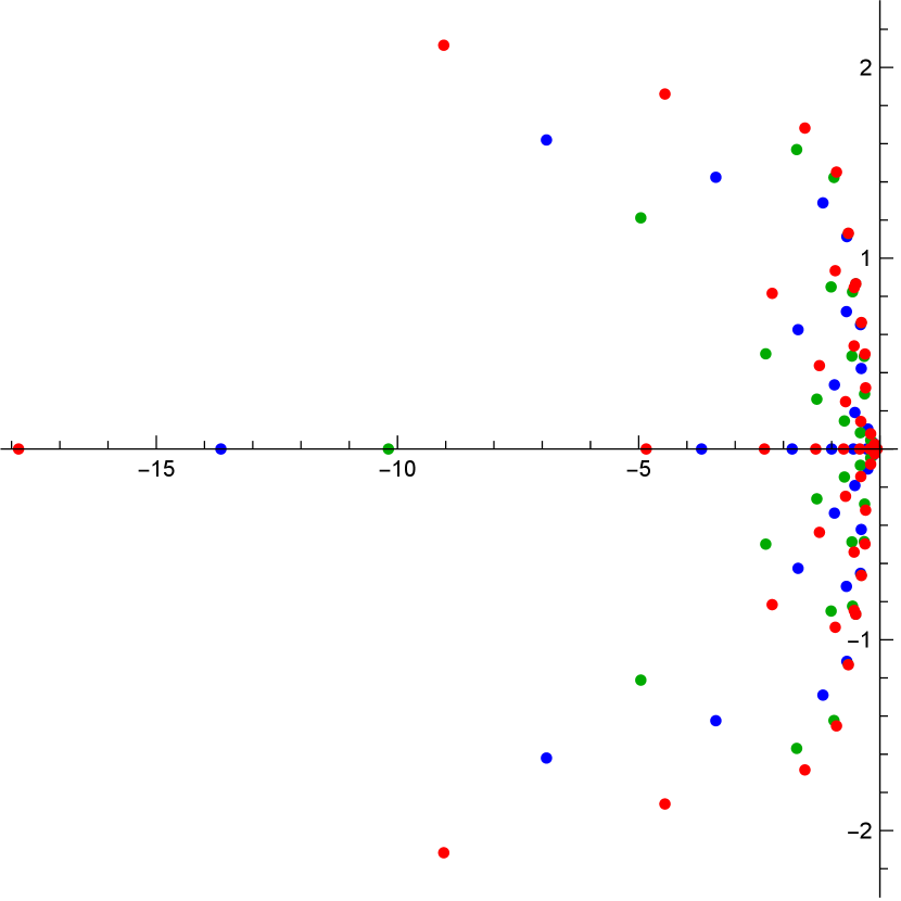
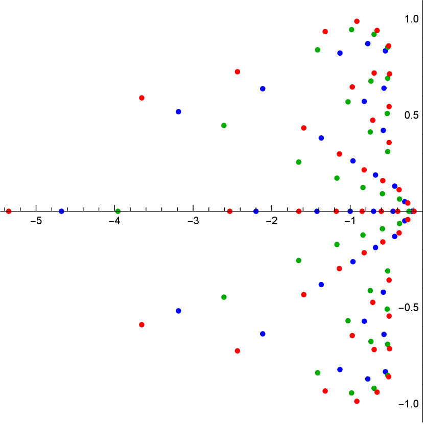
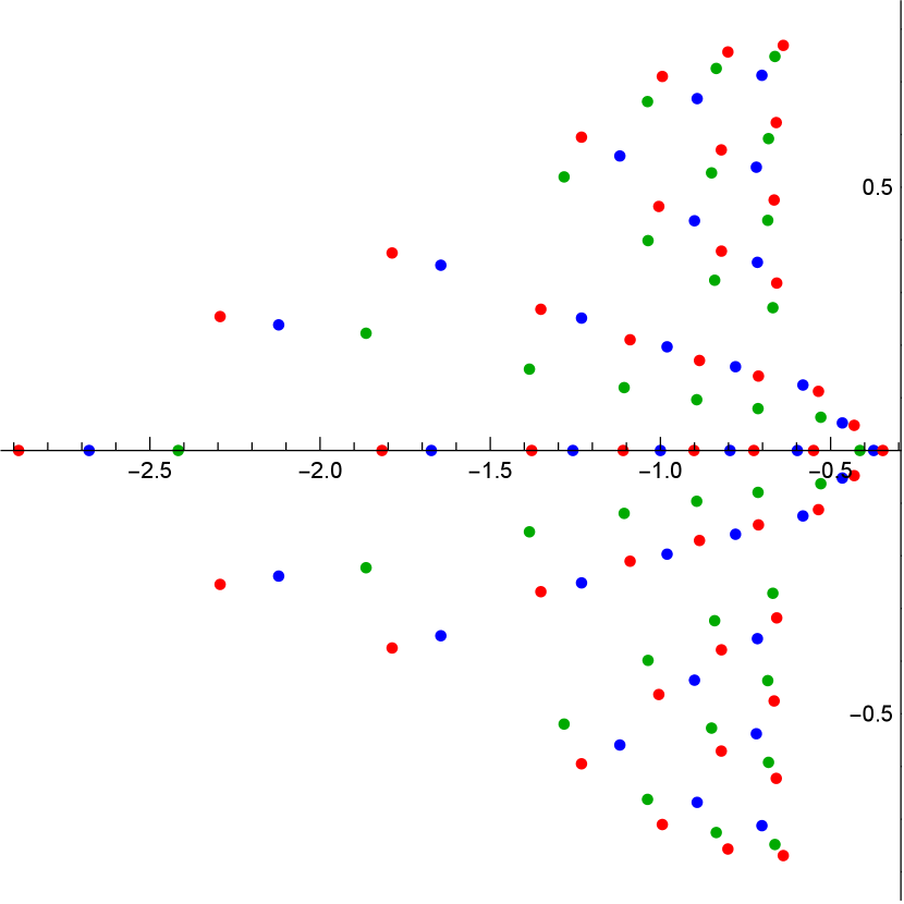
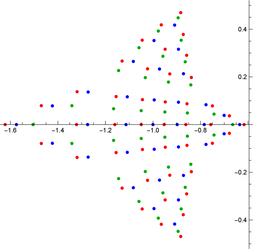
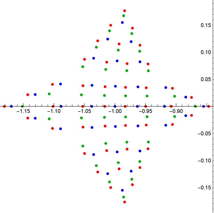
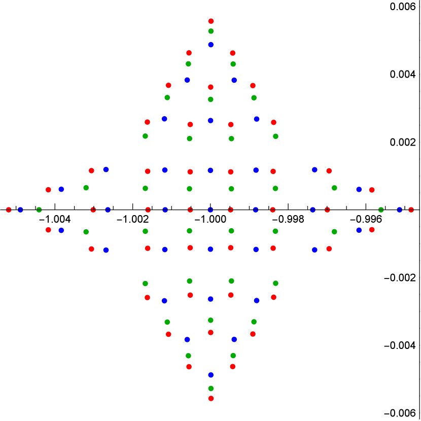
We conclude the section with some graphical representations of the pole distributions of a $q$ -Okamoto rational solution in Figure 2.

6. Conclusion

We have shown that two symmetries $\mathcal{T}_{\pm}$ of $q\textrm{P}_{\textrm{IV}}$ can be lifted to the corresponding Lax pair and monodromy manifold. We have derived four symmetric solutions of $q\textrm{P}_{\textrm{IV}}$ on the discrete time domain $q^{\mathbb{Z}}i$ , which are invariant under $\mathcal{T}_{-}$ . We have further shown that they lead to solvable monodromy problems at the reflection point $t=i$ , which provided an explicit correspondence between the four symmetric solutions and the four points on the monodromy manifold invariant under $\mathcal{T}_{-}$ in Theorem 4.1.

We also studied the family of $q$ -Okamoto rational solutions and showed that they are invariant under both $\mathcal{T}_{+}$ and $\mathcal{T}_{-}$ . We further showed that their simplest member leads to an explicitly solvable monodromy problem in its entire $t$ -domain. We used this to determine the values of the monodromy coordinates on the monodromy manifold for all the $q$ -Okamoto rational solutions. The computation of the monodromy for the $q$ -Okamoto rational solutions in Section 5 could serve as a starting point for deducing similar results for other $q$ -equations.

The pole distributions of the classical Okamoto rational solutions to $\textrm{P}_{\textrm{IV}}$ have been analysed via Riemann-Hilbert methods [buckmiller] and the Nevanlinna theory of branched coverings of the Riemann sphere [masoeroroffelsen]. The extension of such studies to the $q$ -difference Painlevé equations is an open problem.

The results of this paper yield Riemann-Hilbert representations for both the symmetric solutions on discrete time domains and the $q$ -Okamoto rational solutions, through the theory set up in our previous paper [joshiroffelsenrhp]. These can in turn form the basis of the rigorous asymptotic analysis of these solutions, as $t$ grows small or large or some of the parameters tend to infinity.

Appendix A Notation

Define the Pauli matrices

\sigma_{1}=\begin{pmatrix}0&1\\ 1&0\end{pmatrix},\quad\sigma_{2}=\begin{pmatrix}0&-i\\ i&0\end{pmatrix},\quad\sigma_{3}=\begin{pmatrix}1&0\\ 0&-1\end{pmatrix}.

We define the $\mathit{q}$ -Pochhammer symbol by means of the infinite product

(z;q)_{\infty}=\prod_{k=0}^{\infty}{(1-q^{k}z)}\qquad(z\in\mathbb{C}),

which converges locally uniformly in $z$ on $\mathbb{C}$ . In particular $(z;q)_{\infty}$ is an entire function, satisfying

(qz;q)_{\infty}=\frac{1}{1-z}(z;q)_{\infty},

with $(0;q)_{\infty}=1$ and simple zeros on the semi $q$ -spiral $q^{-\mathbb{N}}$ . The $\mathit{q}$ -theta function is defined as

\theta_{q}(z)=(z;q)_{\infty}(q/z;q)_{\infty}\qquad(z\in\mathbb{C}^{*}),

(A.1)

which is analytic on $\mathbb{C}^{*}$ , with essential singularities at $z=0$ and $z=\infty$ and simple zeros on the $q$ -spiral $q^{\mathbb{Z}}$ . It satisfies

\theta_{q}(qz)=-\frac{1}{z}\theta_{q}(z)=\theta_{q}(1/z).

For $n\in\mathbb{N}^{*}$ we denote

	$\displaystyle\theta_{q}(z_{1},\ldots,z_{n})$	$\displaystyle=\theta_{q}(z_{1})\cdot\ldots\cdot\theta_{q}(z_{n}),$
	$\displaystyle(z_{1},\ldots,z_{n};q)_{\infty}$	$\displaystyle=(z_{1};q)_{\infty}\cdot\ldots\cdot(z_{n};q)_{\infty}.$

For conciseness, we will use bars to denote iteration in $t$ . That is, for $f=f(t)$ , we denote $f(q\,t)=\overline{f}$ , and $f(t/q)=\underline{f}$ .

Appendix B Proof of a technical lemma

Proof of Lemma 3.6.

Let $C(z,t)$ be the connection matrix corresponding to the solution $f$ . Let $t_{*}\in q^{\mathbb{Z}}t_{0}$ be such that $f(t_{*})$ is regular. Then the Lax matrix $A(z,t_{*})$ is well-defined at this point and consequently, we have a corresponding connection matrix $C(z,t_{*})$ defined via equation (3.12). Furthermore, using the time-evolution of the connection matrix in equation (3.13), we can thus infer that $C(z,t_{0})$ is also well-defined.

Now suppose, on the contrary, that the corresponding monodromy coordinates,

p_{k}=\pi(C(x_{k},t_{0})),

lie on the curve defined by the cubic equations (3.18). We are going to obtain a contradiction by showing that $C(z,t_{0})$ does not satisfy property c.3. To this end, we will first obtain a general parametrisation of this curve.

Consider the following matrix function,

\mathcal{C}(z)=\begin{pmatrix}C_{1}(z)&C_{2}(z)\\ -C_{1}(-z)&C_{2}(-z)\end{pmatrix},

(B.1)

where

	$\displaystyle C_{1}(z)$	$\displaystyle=\theta_{q}(+z/u,-z/u,z/w),$	$\displaystyle u^{2}w=$	$\displaystyle\frac{1}{qa_{0}^{2}a_{2}}t^{-1},$
	$\displaystyle C_{2}(z)$	$\displaystyle=z\theta_{q}(+z/v,-z/v,z/w),$	$\displaystyle qv^{2}w=$	$\displaystyle\frac{1}{qa_{0}^{2}a_{2}}t^{+1},$

for any choice of $t,w\in\mathbb{C}^{*}$ . This matrix satisfies properties c.1, c.2, c.4, as well as a degenerate version of c.3, namely

|\mathcal{C}(z)|\equiv 0.

The monodromy coordinates, $P_{k}=\pi(\mathcal{C}(x_{k}))$ , $k=1,2,3$ , of this pseudo-connection matrix, read

(P_{1},P_{2},P_{3})=\bigg{(}-\frac{\theta_{q}(+x_{1}/w)}{\theta_{q}(-x_{1}/w)},-\frac{\theta_{q}(+x_{2}/w)}{\theta_{q}(-x_{2}/w)},-\frac{\theta_{q}(+x_{3}/w)}{\theta_{q}(-x_{3}/w)}\bigg{)}.

(B.2)

These monodromy coordinates solve the cubic (3.16) and their expressions are completely independent of $t$ . In other words, they lie on the intersection of cubics (3.16), as $t$ varies in $\mathbb{C}^{*}$ . In particular, these monodromy coordinates must lie on the curve defined by (3.18).

We will show that (B.2) completely parametrises the curve defined by (3.18), as $w$ varies in $\mathbb{C}^{*}$ . Since we have not assumed anything on $(p_{1},p_{2},p_{3})$ , this is equivalent to proving that there exists a $w$ such that

(P_{1},P_{2},P_{3})=(p_{1},p_{2},p_{3}).

(B.3)

Now, the equation

p_{1}=-\frac{\theta_{q}(+x_{1}/w)}{\theta_{q}(-x_{1}/w)},

has two, counting multiplicity, solutions $w_{1,2}$ , on the elliptic curve $\mathbb{C}^{*}/q^{2}$ , related by $w_{2}\equiv qx_{1}^{2}/w_{1}$ modulo multiplication by $q^{2}$ .

For either choice, $w=w_{1}$ or $w=w_{2}$ , we have $p_{1}=P_{1}$ and the pairs $(P_{2},P_{3})$ and $(p_{2},p_{3})$ satisfy the same two equations (3.18), which are quadratic in the remaining variables. In fact, upon fixing the value of $p_{1}$ , (3.18) has two solutions (counting multiplicity), and these two solutions coincide if and only if $w_{1}$ and $w_{2}$ coincide on the elliptic curve $\mathbb{C}^{*}/q^{2}$ . It follows that (B.3) holds for $w=w_{1}$ or $w=w_{2}$ .

We now fix $w$ such that (B.3) holds, set $t=t_{0}$ in (B.1), and consider the quotient

D(z)=C(z,t_{0})^{-1}\mathcal{C}(z).

Since $C(z,t_{0})$ and $\mathcal{C}(z)$ have the same monodromy-coordinate values, $D(z)$ is analytic at $z=\pm x_{k}$ , $k=1,2,3$ and thus forms an analytic matrix function on $\mathbb{C}^{*}$ . Then, by property c.2,

D(qz)=t_{0}^{\sigma_{3}}D(z)t_{0}^{-\sigma_{3}}.

Since $t_{0}^{2}\notin q^{\mathbb{Z}}$ , the only analytic matrix functions satisfying this $q$ -difference equation are constant diagonal matrices, and therefore $D$ is simply a constant diagonal matrix. But then

C(z,t_{0})D=\mathcal{C}(z),

and neither diagonal entry of $D$ can equal zero, as this contradicts equation (B.1), so $|D|\neq 0$ . Hence

|C(z,t_{0})|=|\mathcal{C}(z)|/|D|\equiv 0,

which contradicts property c.3. The lemma follows. ∎

References

q

(A_{2}+A_{1})^{(1)}

q

title=On symmetrical solutions for the first and second Painlevé equations, author=Kitaev, A.V., journal=Zapiski Nauchnykh Seminarov POMI, volume=187, pages=129–138, year=1991, publisher=St. Petersburg Department of Steklov Institute of Mathematics, Russia
author = Joshi, N, author = Kitaev, A.V., journal = Stud. Appl. Math., number = 3, pages = 253–291, publisher = Wiley Online Library, title = On Boutroux’s tritronquée solutions of the first Painlevé equation, volume = 107, year = 2001

q

q

author = Umemura, H., journal = Sugaku Expositions, number = 1, pages = 77–100, publisher = Providence, RI, USA: The Society, c1988-, title = Painlevé equations and classical functions, volume = 11, year = 1998
author = Watson, G.N., title = The continuation of functions defined by generalized hypergeometric series, journal = Trans. Cambridge Phil. Soc., number = 21, pages = 281–299, year = 1910

q

On symmetric solutions of the fourth qq-Painlevé equation

Abstract.

1. Introduction

Definition 1.1.

1.1. Outline

2. Symmetric Solutions

2.1. 𝒯±\mathcal{T}_{\pm} and the continuum limit

2.2. Symmetric Solutions

Definition 2.1.

Lemma 2.2.

Remark 2.3.

3. Symmetries and the linear problem

3.1. The Lax pair

Lemma 3.1.

Proof.

3.2. The connection matrix

Lemma 3.2.

Lemma 3.3.

Lemma 3.4.

Proof.

3.3. Monodromy coordinates

Proposition 3.5.

Proof.

Lemma 3.6.

4. Explicit solvability of the linear problem at a reflection point

Theorem 4.1.

Remark 4.2.

4.1. The model problem

Lemma 4.3.

Proof.

Lemma 4.4.

Proof.

Proposition 4.5.

Proof.

Corollary 4.6.

Remark 4.7.

4.2. Constructing global solutions

Proof of Theorem 4.1.

5. The monodromy problem of the qq-Okamoto rational solutions

Theorem 5.1 (Kajiwara et al. [kajiwaranoumiyamada2001]).

5.1. Solvable monodromy for the seed solution

Remark 5.2.

5.2. Solvable monodromy of the qq-Okamoto rational solutions

6. Conclusion

Appendix A Notation

Appendix B Proof of a technical lemma

Proof of Lemma 3.6.

References

On symmetric solutions of the fourth $q$ -Painlevé equation

2.1. $\mathcal{T}_{\pm}$ and the continuum limit

5. The monodromy problem of the $q$ -Okamoto rational solutions

5.2. Solvable monodromy of the $q$ -Okamoto rational solutions

References

BuckinghamR.J.MillerP.D.Large-Degree Asymptotics of Rational Painlevé-IV Solutions by the Isomonodromy MethodConstr. Approx.562022233–443@article{buckmiller, author = {Buckingham, R.J.}, author = {Miller, P.D.}, title = {{Large-Degree Asymptotics of Rational Painlevé-IV Solutions by the Isomonodromy Method}}, journal = {Constr. Approx.}, volume = {56}, date = {2022}, pages = {233–443}} GasperG.RahmanM.Basic hypergeometric seriesCambridge University Press, Cambridge1990@book{gasper, author = {Gasper, G.}, author = {Rahman, M.}, title = {Basic hypergeometric series}, publisher = {Cambridge University Press, Cambridge}, date = {1990}} JoshiN.RoffelsenP.On the riemann-hilbert problem for a qq-difference painlevé equationComm. Math. Phys.38420211549–585@article{joshiroffelsenrhp, author = {Joshi, N.}, author = {Roffelsen, P.}, title = {On the Riemann-Hilbert problem for a $q$-difference Painlev\'{e} equation}, journal = {Comm. Math. Phys.}, volume = {384}, date = {2021}, number = {1}, pages = {549–585}} JoshiN.NakazonoN.Lax pairs of discrete Painlevé equations: (A2+A1)(1)(A_{2}+A_{1})^{(1)} caseProc. Roy Soc. A.472201606962016@article{joshinobu2016, author = {Joshi, N.}, author = {Nakazono, N.}, title = {Lax pairs of discrete {P}ainlev\'e equations: {$(A_2+A_1)^{(1)}$} case}, journal = {Proc. Roy Soc. A.}, volume = {472}, pages = {20160696}, year = {2016}} JoshiN.NakazonoN.ShiY.Reflection groups and discrete integrable systemsJournal of Integrable Systems11–372016@article{joshinobushi2016, author = {Joshi, N.}, author = {Nakazono, N.}, author = {Shi, Y.}, title = {Reflection groups and discrete integrable systems}, journal = {Journal of Integrable Systems}, volume = {1}, pages = {1–37}, year = {2016}} KajiwaraK.NoumiM.YamadaY.A study on the fourth qq-Painlevé equationJ. Phys. A342001418563–8581@article{kajiwaranoumiyamada2001, author = {Kajiwara, K.}, author = { Noumi, M.}, author = {Yamada, Y.}, title = {A study on the fourth {$q$}-{P}ainlev\'{e} equation}, journal = {J. Phys. A}, volume = {34}, year = {2001}, number = {41}, pages = {8563–8581}} KanekoK.A new solution of the fourth painlevé equation with a solvable monodromyProc. Japan Acad., Ser. A81575–792005The Japan Academy@article{kaneko2005, author = {Kaneko, K.}, title = {A new solution of the fourth Painlev{\'e} equation with a solvable monodromy}, journal = {Proc. Japan Acad., Ser. A}, volume = {81}, number = {5}, pages = {75–79}, year = {2005}, publisher = {The Japan Academy}} KanekoK.OkumuraS.Special solutions of the sixth painleve equation with solvable monodromy2006arXiv:math/0610673@article{pvisymmetric, author = {Kaneko, K.}, author = {Okumura, S.}, title = {Special Solutions of the Sixth Painleve Equation with Solvable Monodromy}, year = {2006}, journal = {arXiv:math/0610673}} @article{kitaev1991symmetrical}