On rising magnetic flux tube and formation of sunspots in a deep domain
Abstract
We investigate the rising flux tube and the formation of sunspots in an unprecedentedly deep computational domain that covers the whole convection zone with a radiative magnetohydrodynamics simulation. Previous calculations had shallow computational boxes ( Mm) and convection zones at a depth of 200 Mm. By using our new numerical code R2D2, we succeed in covering the whole convection zone and reproduce the formation of the sunspot from a simple horizontal flux tube because of the turbulent thermal convection. The main findings are (1) The rising speed of the flux tube is larger than the upward convection velocity because of the low density caused by the magnetic pressure and the suppression of the mixing. (2) The rising speed of the flux tube exceeds 250 m/s at a depth of 18 Mm, while we do not see any clear evidence of the divergent flow 3 hr before the emergence at the solar surface. (3) Initially, the root of the flux tube is filled with the downflows and then the upflow fills the center of the flux tube during the formation of the sunspot. (4) The essential mechanisms for the formation of the sunspot are the coherent inflow and the turbulent transport. (5) The low-temperature region is extended to a depth of at least 40 Mm in the matured sunspot, with the high-temperature region in the center of the flux tube. Some of the findings indicate the importance of the deep computational domain for the flux emergence simulations.
keywords:
Sun: interior – Sun: photosphere – Sun: sunspots1 Introduction
Sunspots are one of the most prominent phenomena at the solar surface. Sunspots have a strong magnetic field ( G), which causes suppression of the convective heat transport and resultant darkening (see review by Borrero & Ichimoto, 2011). The origin of sunspots is thought to be deep in the convection zone (Parker, 1955). The magnetic flux tube generated by the dynamo action is thought to rise to the surface and form sunspots at the solar surface (Zwaan, 1985).
To understand the rising of the flux tube and the formation of sunspots using numerical simulations, realistic physics processes such as radiation, ionization, and thermal convection need to be considered. All of these are fundamentally important, and several numerical simulations of the formation of sunspots have been carried out using these processes. The first numerical simulation for sunspot formation including all these process was performed by Cheung et al. (2010) using a 7.5-Mm deep computational box. The magnetic flux torus is inserted from the bottom boundary kinematically with a certain velocity. They find that the primary mechanism of the formation of sunspots is the turbulent correlation against the mean diverging motion in the central region.
Rempel & Cheung (2014) performed simulations of emerging magnetic flux with a 15-Mm deep calculation domain. They find that the continuous upflow at the bottom boundary prevents the formation of sunspots at the photosphere; thus, they needed to change the boundary condition from the forced upflow to free open during the formation process. Later, Birch et al. (2016) compare their helioseismic observations of the surface divergent flow with Rempel & Cheung (2014)’s calculations with different inserted velocities. Their observations do not find any clear evidence of the divergent flow at 3 hr before the emergence time. In the simulations, the divergence flow 3 hr before the emergence time is seen when the inserted velocity is large at the bottom boundary at a depth of 18 Mm. They conclude that the rising velocity should not be larger than 150 at the bottom boundary not to have clear evidence of the divergent flow against the fluctuation caused by supergranulation.
Stein & Nordlund (2012) performed a sunspot simulation with a 20-Mm box in the vertical direction. The initial magnetic condition is the homogeneous flux sheet, and the turbulent convection spontaneously generates the flux rope and a resulting sunspot pair at the solar surface.
In these simulations, they need to assume the initial condition of the magnetic flux tube or sheet. To exclude this voluntariness, Chen et al. (2017) adopt the bottom boundary condition referred from dynamo calculation (Fan & Fang, 2014). There have been a number of dynamo calculations in which the large-scale magnetic field and cycle are reproduced (Ghizaru et al., 2010; Käpylä et al., 2012; Nelson et al., 2013; Hotta et al., 2016). None of these studies include the photosphere, and the typical top boundary is 30 Mm below the photosphere. Fan & Fang (2014) find spontaneous flux rising in their simulation, but the rising scale is about 800 Mm, which is much larger than what is expected from the photospheric observation. Thus, Chen et al. (2017) rescale the results from the dynamo calculation by a factor of 4–8 in space to fit their photospheric calculation. The time scale and rising speed are also changed from the original dynamo calculation. In addition, the boundary condition is not influenced by what is occurring in the photospheric calculation. They find deep-seated downflow at the bottom boundary with the monolithic structure of the generated sunspot. They find that the converging flow accompanying the downflow collects the magnetic flux.
While the understanding of the formation of sunspots has been significantly improved in the last decade because of the realistic simulations presented, the computational domains of these studies are relatively shallow (<30 Mm) compared with the depth of the convection zone (200 Mm). We would expect some boundary effects on the resulting evolution of the flux tube and sunspots. To minimize the boundary influence to the evolution of the flux tube and a generated sunspot, we need to extend the calculation box. Recently, our new numerical code R2D2 ( Radition and RSST for deep dynamics, where RSST is the reduced speed of sound technique ) succeeds in covering the whole convection zone in a calculation (Hotta et al., 2019). In this study, we carry out a calculation of the rising flux tube with an unprecedentedly deep calculation box that covers the whole convection zone. Recently, Toriumi & Hotta (2019) perform a flux emergence simulation with a 140-Mm deep calculation box using the R2D2 code. In that study, we find spontaneous formation of the delta-type sunspot, which tends to have solar flares. In this study, we investigate the detailed mechanism of the rising of the flux tube and the formation of the sunspot in a deep domain in which the influence of the bottom boundary is expected to be small.
The rest of the paper is structured as follows. Section 2 describes the scheme and the setting of the numerical simulation. Section 3 shows the calculation results of the rising flux tube, formation process, and structure of the matured sunspot. In Section 4, we summarize our results and discuss the differences from previous studies. Future perspectives of flux emergence simulations are also discussed.
2 Model
2.1 Equations
We solve the three-dimensional magnetohydrodynamic (MHD) equations in the Cartesian geometry with the radiation transfer, where the -direction is vertical and the and directions are horizontal. In this study, is the solar surface, which is from the center of the sun. The equations are solved with the R2D2 code. The magnetohydrodynamic equations are expressed as:
| (1) | |||||
| (2) | |||||
| (3) | |||||
| (4) | |||||
| (5) |
where , , , , , , , and are the density, fluid velocity, magnetic field, gas pressure, temperature, entropy, gravitational acceleration, and radiative heating, respectively. The subscript 1 indicates the perturbation from the stationary 1D stratification indicated with subscript 0. Thus, the thermodynamic variables are expressed as:
| (6) | |||||
| (7) | |||||
| (8) |
In this study, we do not assume that the perturbation is smaller than the stationary background stratification, i.e., is not assumed. The background stratification is calculated with the hydrostatic equation with the help of the Model S (Christensen-Dalsgaard et al., 1996). See Appendix A for the details of the calculation procedure.
The equations are solved with the fourth-order spatial derivative (see Appendix B for details) and the four-step Runge–Kutta method for the time integration (Vögler et al., 2005). To maintain the stability of the calculation, we adopt the slope-limited diffusion suggested by Rempel (2014).
We use the equation of state considering the partial ionization effect with the OPAL repository (Rogers et al., 1996). We switch the linear and table equations of state to address the significant change of the perturbation through the convection zone. We evaluate value
| (9) |
If exceeds , we use the table equation of state ; otherwise, the linear equation of state,
| (10) |
is used. and are prepared with the background stratification and only depend on the height (). Regarding the table equation of state, we prepare grid on the density and entropy.
We adopt the RSST (Hotta et al., 2012; Hotta et al., 2015; Iijima et al., 2019) for the equation of continuity to deal with the low Mach number flow in the deep convection zone. By using the RSST, we try to keep the Mach number throughout the convection zone. To this end, we set the RSST factor,
| (11) |
Here, we adopt . and are the density and the speed of sound around the base of the convection zone, respectively. is the local adiabatic speed of sound. When the energy flux is fixed, the convection velocity scales with in the mixing length theory. This setting approximately maintains the Mach number. Fig. 1 shows the RSST factor (panel a) and the reduced speed of sound (panel b). Hotta et al. (2012) show that if the Mach number estimated with the reduced speed of sound is smaller than 0.7, the RSST cause no side effect on the result.

We limit the Alfven velocity to 40 to deal with low- region above the photosphere Rempel et al. (2009b). This does not affect what is occurring at the photosphere.
The radiative heating is calculated with the radiative transfer equation; the details are shown in Appendix C.
We calculate the thermal convection with the top boundary at for 90 days. The thermal convection around the photosphere is very fast, and we exclude this layer for accelerating the calculation. Then, we include the photosphere with the top boundary at 700 km above the photosphere and continue the calculation for 5 days. This procedure is justified because the existence of the photosphere does not change the deep structure (Hotta et al., 2019).
The calculation domain extends 98.304 Mm horizontally for and directions. The vertical calculation extent is from the base of the convection zone and to . The number of grid points in each horizontal direction is 1024, and the grid spacing is 96 km, and this is acceptable to resolve the photosphere. In the vertical direction, we use 512 grid points and nonuniform grid spacing, and this is 48 km around the photosphere and 900 km around the base of the convection zone.
2.2 Initial condition
We adopt the Lundquist solution (Lundquist, 1950) for the linear force-free flux tube as follows:
| (12) | |||||
| (13) | |||||
| (14) | |||||
| (15) | |||||
| (16) | |||||
| (17) |
where is the first root of , and is the radius of the flux tube. and are the Bessel functions. Here, we adopt , i.e., the initial magnetic flux tube is located about 35 Mm below the photosphere and for the magnetic field strength at the center of the flux tube. This leads to a total flux of . is an arbitrary parameter with which the horizontal location of the flux tube is determined. With our choice, the initial flux tube is located in the center of the computational domain. Fig. 2 shows the initial flux tube condition at . The initial flux tube is caught by the two coherent downflows. Note that the left downflow is larger and more coherent. Because the initial magnetic flux tube is force-free, we do not change any thermodynamic variable, i.e., the density, pressure, or entropy from the prepared hydrodynamic calculation. Thus, the magnetic flux initially does not have any buoyancy by the magnetic field, but the inertia of the convective flow can distort the magnetic flux tube.

3 Results
3.1 Magnetic flux and area
Fig. 3 shows the temporal evolution of unsigned magnetic flux on surface (panel a) and the area of the sunspot (panel b). In Fig. 3a, the black line shows the unsigned magnetic flux integrated over all horizontal domains. The red and blue lines show the unsigned magnetic flux with the emergent intensity less than 80% and 50% of the averaged quiet sun intensity , respectively. Fig. 3b shows the area with the emergent intensity less than (red) and (blue). For making Fig. 3b, we use the Gaussian filter with a width of 1 Mm. The unsigned magnetic flux reaches its maximum of at hr. We follow the definition of the emergence time suggested by Leka et al. (2013), in which the unsigned magnetic flux reaches 10% of the maximum magnetic flux. The emergence time in this calculation is hr. After the magnetic flux reaches its maximum, the magnetic flux begins to decrease. Around , almost all the magnetic flux in the sunspot disappears, leading to approximate emergence and decay rates () of and , respectively. These values are similar to those in Rempel & Cheung (2014). We note that they determine the rising speed of the flux tube at the bottom boundary, while the combination of the convection and the magnetic field determines the rising property in this calculation.
Compared with the observations, Otsuji et al. (2011) and Norton et al. (2017) show the relation of the maximum sunspot flux and the emergence rate as and , where both are in the unit of . The maximum flux of the current simulation leads to and with using Otsuji et al. (2011) and Norton et al. (2017) relations, respectively. In addition, Namekata et al. (2019) show that the 95% confidence interval of the emergence rate reaches with . Compared with these observational results, this numerical simulation shows a slightly larger emergence rate.
Regarding the decay rate of the sunspot, Hathaway & Choudhary (2008) show the observational relation between the sunspot area and the dissipation rate as . We assume that the mean magnetic field strength is 2000 G, which is used in Namekata et al. (2019). This relation leads to , which is consistent with the simulation in this study. Fig. 3b shows that the area of the sunspot reaches its maximum at hr and that the area decreases to zero at hr. This leads to the decay rate of . The Hathaway & Choudhary (2008) relation leads to for our case. Also, in terms of area, the calculation result is consistent with the observation.
3.2 Overall evolution
Figs. 4 and 5 show the emergent intensity and line-of-sight magnetic field at surface, respectively. Around the emergence time hr, we begin to see small pores in the intensity map (Fig. 4b) and a diffused pattern in the magnetic field map (Fig. 5b). As time progresses, the small pores merge and construct the large-scale structure. At , we observe elongated granules between the positive and negative spots (Fig. 4c and 5c). When the photospheric magnetic flux reaches its maximum, a coherent sunspot appears (Fig. 4d and 5d). While we see some evidence of the penumbra around the sunspot, the reproduced penumbra is much less prominent than the observation. Rempel (2012) shows that the existence of the penumbra is significantly affected by the top boundary condition. Here, we use the potential magnetic field condition, while Rempel (2012) argues that the horizontally inclined magnetic field at the top boundary is required for a prominent penumbra. We also note that Rempel et al. (2009a) show that the penumbra can be observed between two sunspots because the horizontal magnetic field is expected between them. In this study, the matured sunspots are far apart from each other, and even the penumbra between the sunspot pair cannot be observed.
After the magnetic flux reaches its maximum, the sunspots begin to lose their magnetic flux. At , the right sunspot loses significant flux, while the left sunspot keeps a coherent shape with some bright features in the umbra (Fig. 5e). At hr, almost all the magnetic flux disappears from the umbra (Fig. 4f and 5f).
Fig. 6 shows the three-dimensional structure of the magnetic field deep in the convection zone. At , the magnetic field shows an -shape structure with two anchoring downflows and a broad upflow in the center region (Fig. 6b). At (Fig. 6c), which is around the emergence time, a significant fraction of the magnetic flux reaches the near-surface layer (). At (Fig. 6d), which is around the time of the maximum photospheric magnetic flux, the root of the left sunspot reaches a depth of around 80 Mm, while the root of the right sunspot remains at a depth of around 30 Mm. Below the photosphere, the magnetic field of the sunspot is mostly vertical. At hr (Fig.6e), the sunspots begin to decay; at the same time, the subsurface structure is destroyed. At hr (Fig. 6f), when the sunspot disappears almost completely, most of the flux is transported downward, and coherent features can still be seen in the deep region below a depth of 60 Mm.
The Coriolis force is an important factor for the tilt angle (Wang & Sheeley, 1991) and the asymmetry of the sunspot pair (D’Silva & Choudhuri, 1993). Cheung et al. (2010) show an almost symmetric sunspot pair because of their almost symmetric initial condition and setting. Rempel & Cheung (2014) show an asymmetric sunspot pair resulting from the horizontal flow mimicking the Coriolis force-induced flow. Chen et al. (2017) also show asymmetry resulting from the boundary condition motivated by the dynamo calculation influenced by the Coriolis force. While the Coriolis force must be importanat to generate a statistical trend of the sunspot pair feature (Weber et al., 2011), our calculation without the Coriolis force can also cause some asymmetry in the sunspot pair. The asymmetry in this study reflects the convection flow structure in the deep convection zone. The initial condition (Fig. 2) shows that the left downflow has a more circular shape than does the right downflow, which shows an elongated feature. Interestingly, the emerging sunspot follows this morphology. Fig. 7 shows the flow and magnetic structure in deep layers at hr. Color and line contours show the vertical velocity () and magnetic field (), respectively. At a depth of at least 30 Mm (Fig. 7b), we can still observe the asymmetry of the magnetic feature, i.e., the positive magnetic feature (solid line) shows the circular shape, while the negative feature (dashed line) is elongated. In the deeper layer, the positive feature maintains a circular shape. The negative feature crosses the boundary and reaches the other side indicated with a black arrow in Fig. 7c because of the periodic boundary condition. At a depth of 50 Mm, the negative feature has a circular shape (black arrow in Fig. 7d). We note that the time scale of the convection at 50 Mm depth is about 5 days, and the structure of the magnetic flux tube has not been distorted well at this depth. This result indicates that the shape of the sunspot is influenced by the deep convection structure at least 30 Mm below the photosphere.


3.3 Rising mechanism of flux tube
In this section, we investigate the rising process of the flux tube mainly around the center region ( Mm). Fig. 8 shows the temporal evolution of the rising flux tube. The left and right panels show the vertical velocity and Alfven velocity of the axial field , respectively. To investigate the motion of the flux tube, we adopt the following definition of the center of the flux tube. Basically, we use a clumping method. We detect clumps of the region having an Alfven velocity beyond a given threshold. With iteration, we survey the threshold with which the largest clump has a magnetic flux of , where the magnetic flux is estimated with . The largest clump () in each time step is defined as the rising flux tube. The center of the flux tube is defined as follows:
| (18) | |||||
| (19) |
The boundary and center of the flux tube are shown with black lines and black crosses in Fig. 8, respectively. The time evolution of the center of the flux tube is shown in Fig. 9. Fig. 9a shows the vertical position of the center of flux tube . In the beginning, the rising speed increases with time, when the flux tube reaches the solar surface, the speed is reduced. The time profile of the vertical position is not smooth because of sudden merging and splitting. To evaluate the rising speed, we use a Savitzky–Golay filter for the vertical position, which is shown as the red line in Fig. 9a. By using the filtered profile of the vertical position, we estimate the rising speed of the center of the flux tube. The black line in Fig. 9b shows the rising speed of the flux tube. The red line shows the root-mean-square (RMS) upflow convection velocity in a hydrodynamic run, i.e., without the magnetic field. We note that the downflow convection velocity is typically larger than the upflow velocity. The blue line shows the mean Alfven velocity in the flux tube. In the beginning, the rising speed is almost the same as the upward convection velocity. This is natural because the initial flux tube is force-free and the flux tube needs to obey the convective flow. As time progresses, the rising speed exceeds the convection velocity, indicating some contribution of the magnetic field to the rising process. Even at the end of the rising process, the rising speed does not reach the local Alfven velocity. This result indicates that the rising process is neither a pure magnetic nor a pure convective process.
To understand the rising mechanism, we investigate the vertical equation of motion. Fig. 10a shows the vertical forces averaged in the flux tube. Before evaluating the equation of motion, we filtered out the sound waves in the phase space (Georgobiani et al., 2007). The equation of motion in the vertical direction is the following:
| (20) |
The red and blue lines in Fig. 10a show the buoyancy () and Lorentz force (), respectively. The moving flux tube can be roughly regarded as a Lagrangean parcel in the plane. Only the contribution from the inertia term () to the motion of the rising flux tube is (). The black line is the sum of these terms. The buoyancy and total force direct upward during the rising process, while the Lorentz force directs downward. The main contribution of the Lorentz force is magnetic tension. The roots of the magnetic flux are anchored in the deep layer; thus, the magnetic tension in the rising part directs downward. Fig. 10b shows the mean normalized density, pressure, and entropy in the flux tube. The normalization procedure, i.e., the tilde, for quantities are defined as follows:
| (21) | |||||
| (22) | |||||
| (23) |
where and are the horizontal average and RMS value of a quantity in the calculation without the magnetic field, respectively. After normalization, the density, pressure, and entropy are related as . We also note that because is negative, the negative value of corresponds to a positive perturbation of the entropy and vice versa. The result shows that the mean normalized density in the flux tube is significantly low (the perturbation is 1.7 times larger than the RMS value); this is the primary driver of the rising flux tube. There are two contributions to the low density in the flux tube. The first is the low pressure caused by the magnetic pressure. After the rising starts, the twist becomes relaxed and the force-free balance is destroyed. Then, the gas pressure gradient force plays a role in maintaining the flux tube and decreasing the gas pressure in the flux tube. Because the initial flux tube is force-free, the magnetic tension plays a role in balancing the magnetic pressure, even during the rising process; thus, the gas pressure is not significantly low in this case. The other contribution to the low density is the high entropy maintained by the suppression of the mixing. The initial magnetic flux tube is located in the upflow region and has higher entropy than does the surrounding plasma. As seen in Fig. 8c and d, the magnetic field suppresses the mixing between upflows and downflows. In an ordinary medium in the convection zone, the upflow warm medium is mixed in a mixing length and loses its high entropy, but this magnetic flux tube can avoid this process and maintain high entropy, leading to continuously low density in the flux tube and further acceleration. Fig. 10b shows that the high entropy is the main contribution to the low density in the flux tube.


3.4 Surface flow prior to emergence time
In this section, we investigate the divergent flow prior to emergence time to compare the results with Birch et al. (2016), in which clear divergent flow is not seen at 3 hr before the flux emergence.
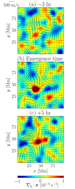
To this end, we follow a similar procedure to that of Birch et al. (2016). We take the divergence of the horizontal flow at surface and the Gaussian filter with a 6-Mm window. Fig. 11 shows the horizontal divergence at surface at and 37, and 42 hr. The standard error of the distribution is , and the black line in Fig. 11 shows the 3 value. We again note that hr is the emergence time. Panels a and c are 5 hr after and 3 hr before the emergence time. While we see a clear divergent flow at and after the emergence time (panels b and c), we do not see it 3 hr before the emergence time (panel a). This result is consistent with the observation of Birch et al. (2016). By contrast, the rising speed of the flux tube exceeds at a depth of 18 Mm, while Birch et al. (2016) suggest that the rising speed is no larger than to avoid divergent flow prior to the emergence time.
Fig. 12 shows the temporal evolution of the horizontal divergence at surface. The black and red lines show the maximum and top 1% value of the divergent flow, respectively. This also indicates that the clear evidence of the divergent flow is seen at only 1 hr before the emergence time.

3.5 Flow in flux tube
In this section, we investigate the flow in the flux tube during the flux emergence process. First, we discuss the vertical flow at Mm in detail. Then, we discuss the flow at different heights. Fig. 13 shows the temporal evolution of the vertical flow and the density in the flux tube. From this section, we focus on the left coherent positive sunspot. Because the root of the sunspot is created with the downflow from the horizontal magnetic flux tube, the root is initially filled with the downflow (Fig. 13a: hr). This is somewhat consistent with Chen et al. (2017), in which the strong magnetic concentration occurs at a coherent downflow in the deep layer. A difference is seen in the following evolution. The flow in the flux tube changes signs around hr in Fig. 13c. After the sunspot is formed (Fig. 13e: hr), the flux tube is filled with the upflow. During this process, the flux tube is filled with the low-density medium (Figs. 13b, d, and f).
Here, we define the flux tube as the largest clump in which the vertical magnetic field exceeds the threshold value of 7000 G. Fig. 14a shows the temporal evolution of the mean vertical flow in the flux tube. In the beginning, the flux tube is filled with the downflow. Around hr, the downflow stops increasing in amplitude. Around hr, the vertical flow changes signs. Afterward, the amplitude of the upflow increases continuously. Fig. 14b shows the force balance in the flux tube. The red and blue lines show the buoyancy and the Lorentz force, respectively. The flux tube roughly acts as the Lagrangean parcel in the plane. Thus, for the total dynamics, the contribution from the inertia term is the vertical inertia term . The black line in Fig. 14b shows the sum of the buoyancy, Lorentz force, and vertical inertia terms. The total force is consistent with the temporal evolution of the vertical velocity in the flux tube. Around hr, the total force changes its sign and keeps the positive value after that. The main driver of the upflow in the flux tube is the buoyancy. Fig. 14c shows the normalized density, pressure, and entropy averaged in the flux tube (see eqs. (21)–(23)). In this case, the main contribution of the low density is the low gas pressure caused by the adiabatic expansion from the Lorentz force.
Fig. 15 shows the azimuthally averaged values in the polar coordinate. Because the generated sunspot and its flux tube are tangling along the vertical direction, different heights cannot share the same origin as the polar coordinate. Thus, we define the origin of the polar coordinate at every depth separately. We adopt the following procedure.
-
1.
We estimate the magnetic flux of the positive vertical magnetic field in the left half of the computational domain ().
-
2.
The threshold value of the magnetic flux () is of .
-
3.
We search the critical value for the vertical magnetic field with which the largest clump has a vertical magnetic flux of , where the definition of the clump is the continuous region in which the vertical magnetic field exceeds the critical value. The flux tube is identified with .
-
4.
The origin of the polar coordinate at depth is defined with the following:
(24) (25) -
5.
If is smaller than , we use the origin of the polar coordinate defined at a place one grid below.
-
6.
The vertical profile of the origin of the polar coordinate is not smooth. We obtain the smooth profile of the origin of the polar coordinate with the Savitzky– Golay filter. The filtered profile is used for the origin of the polar coordinate in the following analyses.
Fig. 15 shows the azimuthally averaged profile of the vertical velocity (Fig. 15a) and the normalized density (Fig. 15b) at hr, where the parenthesis shows the azimuthal average at constant radius . The finding at a depth of 30 Mm is applicable to different depths. Except for the near-surface layer ( Mm), the center of the flux tube is filled with the upflow, surrounded by the coherent downflow in the outer side of the flux tube. The coherent upflow corresponds to low density (Fig. 15b), indicating that the driving mechanism of the upflow is the buoyancy.


3.6 Formation mechanism of sunspot
In this section, we discuss the formation mechanism of sunspots. The most important process for the formation of sunspots is the collection of the magnetic flux toward the center region. As discussed in Cheung et al. (2010), the temporal evolution of the magnetic flux is expressed as follows:
| (26) | |||||
where area is a circular area with fixed radius at height , and shows the azimuthal average. Cheung et al. (2010) suggests that the essential term for collecting the magnetic flux at the photosphere is . This is caused by the mass loss at the highly inclined field (see Fig. 8 in Cheung et al. (2010)).
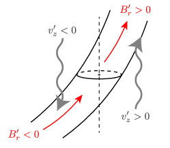
Fig. 16 shows the azimuthally averaged radial velocity (: panel a) and one of the turbulent induction terms (: panel b). The definition of the origin of the polar coordinate is the same as that in Section 3.5. The values are averaged between and 37 hr, and this range is around the emergence time, which is before the formation of the sunspot. At this time, the sunspot location in the near-surface is filled with the outflow from the center to the outside, which is the negative effect for the generation of the sunspot. Among the induction terms, the most important contribution is from . In Fig. 16b, this term is positive in the magnetic flux. This can be explained with Fig. 17. The horizontal magnetic field with positive can be regarded as a negative radial magnetic field () in the downflow side (). In the upflow region (), the radial magnetic field is positive (). Both cause a positive correlation, meaning that before the formation of the sunspot, the shear of the downflow and the upflow are the most important mechanisms for the generation of the vertical magnetic flux.
Fig. 18 shows the azimuthally averaged flows and induction terms averaged between and 53 hr, i.e., during the formation of sunspots. We find a strong coherent downflow and inflow at the near-surface layer ( Mm) in the center (Figs. 18a and b, indicated with a dash-dot line). This makes an important contribution to the collection of the vertical magnetic flux (Fig. 18c). This flow is transient and continues less than 10 hr. While the existence of this downflow and inflow is not reported in Cheung et al. (2010), Rempel & Cheung (2014) show its importance (see their Fig. 11). The treatment of the bottom boundary would be important for the flow for calculations without the deep layer.
In the outer side of the sunspot, we see the Evershed-like outflow in the near-surface layer ( Mm, indicated with a dashed line in Fig. 18b), which does not contribute to the loss of the vertical magnetic flux in this phase, because the Evershed flow and the magnetic field line are roughly aligned (Fig. 18c). In the deeper layer, the sunspot core is filled with weak outflow, reducing the vertical magnetic flux in this phase (indicated with a doted line in Fig. 18b). In the outer area, we also see weak inflow that does not play any role in the collection of the vertical flux (indicated with a dash-dot-dot line in Fig. 18b).
The most important contribution of the formation of the sunspot in the outer region is a turbulent induction term (), which is consistent with Cheung et al. (2010) and Rempel & Cheung (2014). The turbulent induction term () has a negative value in the deeper layer ( Mm). Even the sum of all the induction terms has a negative value in the deep layer during the formation of the sunspot at the solar surface. Consequently, the decay of the sunspot starts during its formation.


3.7 Sunspot structure
In this section, we report the overall flow structure of the matured sunspot in comparison with the sunspot during formation.
Fig. 19 shows the azimuthally averaged flows and induction terms in the same manner as Fig. 18, but the values are averaged between to 69 hr, in which the unsigned magnetic flux has its maximum value. Compared with the sunspot during formation, the strong coherent downflow and inflow in the near-surface layer disappear (Figs. 19a and b), whereas, weak downflow and inflow are seen in the near-surface layer (). Nonetheless, the weak inflow still contribute to collecting the vertical magnetic flux in the near-surface layer (Fig. 19c) . In the deep layer ( to Mm), the root of the sunspot is filled with the outflow, which is connected to the Evershed-like flow in the outer area in the near-surface. This outflow in the middle layer makes an important contribution to the decay of the sunspot. In the deeper layer ( Mm), the center of the flux tube is filled with the upflow, as discussed in Section 3.5. This upflow is also connected to the outflow in the middle layer and the Evershed-like flow in the near-surface. We see coherent inflow in the outside the flux tube (Fig. 19b), which is connected to the downflow in the outer layer of the flux tube in the deeper layer. This coherent inflow makes a significant contribution to the collection of the magnetic flux, i.e., the maintenance of the sunspot. The turbulent induction term still makes a significant contribution to the maintenance of the sunspot in the near-surface layer, even if the sunspot is matured.
Fig. 20 shows the azimuthally averaged normalized temperature averaged between and 53 hr (panel a, during the formation) and and 69 hr (panel b, matured sunspot), where . As the formation process of the sunspot proceeds, the low-temperature region expands because of the suppression of the convective energy transport and the radiative cooling at the photosphere. In both cases, we see a high-temperature region in the center of the flux tube below a depth of Mm. While the phase of the sunspot formation is different in panels a and b, the depth where the temperature changes from high to low does not change. In the matured sunspot, the coherent low-temperature region continues to a depth of 40 Mm.


4 Summary and Discussion
In this study, we perform a numerical experiment of the flux emergence in an unprecedentedly deep domain that covers the whole convection zone from the base to the surface. The main purpose of this setting is to minimize the influence of the bottom boundary condition on the rising of the flux tube, formation of the sunspot, and internal structure of the generated sunspot.
The main findings of this study are summarized as follows:
-
•
The rising speed of the flux tube tends to be larger than the typical upward convection velocity because of the low density caused by the magnetic pressure and suppression of mixing.
-
•
The rising speed of the flux tube exceeds at a depth of 18 Mm, while no clear evidence of the divergent flow 3 hr before the emergence at the solar surface is seen.
-
•
Initially, the root of the flux tube is filled with the downflows, and then the upflow fills the center of the flux tube during the formation of the sunspot because of the low density.
-
•
The essential mechanisms for the formation of the sunspot are the coherent inflow in the central region and the turbulent correlation in the outer region.
-
•
The low-temperature region is extended to a depth of at least of 40 Mm in the matured sunspot, with the high-temperature region in the center of the flux tube.
Fig. 21 summarizes the flow and temperature structure of the sunspot during the formation (panel a) and matured phase (panel b). A large difference in the sunspot structure between the two phases is the strong coherent downflow/inflow to the center of the sunspot down to a depth of 15 Mm during its formation. This downflow is significantly weakened in the matured sunspot and extends only 5 Mm further. The other difference between the two phases is the temperature structure. During the formation, the low-temperature region is mainly seen up to a depth of 10 Mm (some cooling is still seen at a depth of Mm); a coherent low-temperature region is seen down to a depth of 40 Mm surrounding the high-temperature region in the center of the flux tube.

4.1 Reduced Speed of Sound Technique
As discussed in Hotta et al. (2012), we need to keep the Mach number smaller than 0.7 in order to avoid the influence of the RSST. In this study, we keep the Mach number smaller than 0.1 when the RSST is used. Fig. 22 shows the RMS velocity in the hydrodynamic calculation without the magnetic field (panel a) and the Mach number estimated with the reduced speed of sound (panel b). The Mach number is always smaller than 0.1 at locations where the RSST is used (indicated with the dashed line in Fig 22b). Phenomena related with the magnetic field, i.e., the flux emergence and sunspot formation, occurs in a similar time scale as the thermal convection. For example, Fig. 13 shows that the up- and downflow are typically 200–300 , where the reduced speed of sound at z=-30 Mm is about 4 . Thus the Mach number is smaller than 0.1 and we do not expect any significant influence of the RSST on the result shown in this paper.

4.2 Computational domain
In this study, we prepare an unprecedentedly deep computational domain to minimize the bottom boundary influence. This also has a possible drawback on the convection structure. It is known that numerical simulations tend to overestimate the large-scale (> 30 Mm) convection energy in the deep convection zone (Hanasoge et al., 2012; Lord et al., 2014). To reduce the power on a larger scale than the supergranulation, we intentionally prepare the small box in the horizontal direction of 100 Mm (see also Toriumi & Hotta, 2019). This setting causes another side effect. Because of the insufficient horizontal box size and the periodic boundary condition, a generated sunspot is close to the sunspot on the other side. We expect that the calculation results in this study are not an evolution of the single isolated sunspot pair, but rather, the sequence of the sunspot pairs. This fact mainly influences the decay of the sunspot, and we do not discuss this effect in detail in this study.
4.3 Emergence rate
In this study, the emergence rate of the magnetic flux is , which is slightly larger than the 95% confidence interval (, see Section 3.2) suggested by Namekata et al. (2019). There are several possible reasons for this discrepancy. The emergence rate would be determined by the rising speed and the structure of the magnetic flux tube. A fast-rising and intense structure of the flux tube tends to cause a high emergence rate. In this study, we find that the rising speed of the flux tube is not purely determined by the thermal convection; the magnetic effect is also important. Thus, there would be an appropriate initial setting of the magnetic flux tube for reproducing the emergence rate consistent with the observation. Parameter surveys for the initial setting of the flux tube should therefore be carried out in a future study.
By contrast, the number of observations is insufficient to conclude that our emergence rate is larger than reality. There are only several estimations of the emergence rate for the magnetic flux larger than (Toriumi et al., 2014). For example, Sun & Norton (2017) show for an instantaneous emergence rate. More observations are needed to identify the most probable flux tube structure in the deep convection zone.
4.4 Comparison with previous studies
4.4.1 Divergent flow prior to flux emergence
In this study, we find that the rising speed of the flux tube exceeds at a depth of 18 Mm, while we do not see any clear evidence of the divergent flow 3 hr before the emergence time. This is inconsistent with Birch et al. (2016), who argue that the rising speed should not be larger than to have divergent flow at that time. This discrepancy can be caused by the settings in previous studies (Cheung et al., 2010; Rempel & Cheung, 2014). In those studies, a magnetic flux tube has to be inserted kinematically from the bottom boundary because of the shallow calculation box. The speed of the rising flux tube is determined at the bottom boundary, and most of the flux tube has upward velocity. In this study, the flow structure of the flux tube is physically determined. The rising part of the flux tube has upflow, and its root initially has downflow. This natural determination of the rising speed would reduce the influence on the photosphere, i.e., the divergent flow. The constraints on the rising flux tube should be investigated in a deeper computational box, where the interaction of the convection and the magnetic field automatically determines the dynamics of the flux tube.
4.4.2 Upflow in flux tube
The other difference from previous studies is the upflow in the central region of the flux tube. Chen et al. (2017) found that the flux tube of the sunspot is filled with coherent downflow (see Fig. 11 in their work). In their study, they use the data from the dynamo calculation (Fan & Fang, 2014). They also find that the downflow region is the place for the sunspot because the converging flow to the downflow collects the magnetic flux. The flow structure does not change even after the sunspot is formed because the boundary condition is provided. In our study, we do not expect any boundary influence on the evolution of the flow in the flux tube, and the upflow in the central region with low density is a natural consequence of the magnetohydrodynamic process.
Zhao & Kosovichev (2003) show the internal flow structure beneath the sunspot using the local helioseismology. They find converging motion with the downflow in the near-surface layer (depths of Mm) and diverging motion with the upflow in the deeper layer (depths of Mm). Our result for matured sunspots has a consistent flow structure (see Fig. 19). In addition, Fig. 4 of Zhao & Kosovichev (2003) shows that the downflow and upflow are surrounded by the upflow and downflow, respectively, but this information is not explicitly mentioned in the paper. This feature is also consistent with our calculation.
4.5 Future perspective
Previously, flux emergence simulations in the deep convection zone with a thin-flux tube (D’Silva & Choudhuri, 1993; Moreno-Insertis et al., 1995), anelastic approximation (Fan, 2008; Weber et al., 2011), RSST (Hotta & Yokoyama, 2012), and simulations around the solar surface (Cheung et al., 2010; Rempel & Cheung, 2014; Chen et al., 2017) were almost completely separated. Our approach using the R2D2 code sheds light on connecting these two regions. This is an integral part of both the solar dynamo and the formation of the sunspot. Even in the simulation in this study with the computational domain of the whole convection zone, we still assume the initial magnetic flux tube condition because we have a very low vertical resolution in the deep convection zone (). To maintain the magnetic flux of the magnetic flux tube during the rising process from the base of the convection zone to the surface, we need to prepare a high resolution even in the deep convection zone (Cheung et al., 2006). By using the current numerical resources, we are unable to achieve this purpose; however, we will soon be able to perform these types of calculations using next-generation supercomputers, such as Fugaku in Japan. In future studies, we plan to connect dynamo calculation and sunspot formation simulation in a calculation. This approach is expected to reveal the formation process of sunspots in a more self-consistent manner.
Acknowledgments
The authors would like to thank the anonymous referee for the great suggestions. The authors are grateful to Kousuke Namekata for providing the detailed relation of the sunspot flux and the emergence rate. The results were obtained using the K computer at the RIKEN Advanced Institute for Computational Science (proposal Nos. hp190070, hp190183, hp180042, and ra000008). This work was supported by MEXT/JSPS KAKENHI grant Nos. JP19K14756, JP18H04436, JP16K17655, and JP15H05816. This research was supported by MEXT as Exploratory Challenge on Post-K Computer (Elucidation of the Birth of Exoplanets [Second Earth] and the Environmental Variations of Planets in the Solar System) and the Project for Solar-Terrestrial Environment Prediction.
Appendix A Background stratification
For the background stratification of , , , and the other related variables, we use Model S (Christensen-Dalsgaard et al., 1996). Model S does not solve the entropy equation, and the entropy profile is not smooth. By contrast, in this study, the entropy equation is solved, and the tiny variation of the entropy is essential for the thermal convection property. To overcome this difficulty, we recalculate the hydrostatic equation with the help of the Model S. The hydrostatic equation is as follows:
| (27) |
We adopt the value of the gravitational acceleration from the Model S, and we need to specify the distribution of the temperature or the entropy to relate the pressure and the density . We divide the solar convection zone into two parts at . In the deep part, the entropy gradient is small, and we can regard it as adiabatic stratification. Thus, in this region, we adopt a constant value of the entropy at in Model S.
In the upper part of the convection zone (), the entropy gradient is significantly large. To obtain the smooth profile of the entropy gradient around the photosphere, we follow the following procedure:
-
1.
Calculate the entropy gradient using the entropy of the Model S.
-
2.
Use the Savitzky–Golay filter for the entropy gradient to obtain a smooth profile.
-
3.
Solve the hydrostatic equation using the filtered profile.

The black line in Fig. 23 shows the calculated entropy gradient in Model S. To reduce the jaggy feature in the entropy gradient, we use the Savitzky–Golay filter. The red line in Fig. 23 shows the filtered entropy gradient
In addition, the top boundary of the Model S is about 500 km above the photosphere. We extend the stratification with the gravitational acceleration and constant temperature, where we again note that corresponds to the surface of the sun.
Appendix B Fourth-order derivative for inhomogeneous grid
In this study, we adopt inhomogeneous grid spacing in the vertical direction . To maintain the accuracy of the spatial derivative of the quantities, we adopt a general fourth-order formulation for inhomogeneous grid spacing as follows:
| (28) | |||||
| (29) | |||||
| (30) | |||||
| (31) |
The first derivative of a quantity () can be expressed as follows:
Appendix C Radiation transfer
To evaluate the heat and the cooling of the radiation ( in Eq. (4)), we solve the radiation transfer equation.
| (33) |
where is the radiative intensity, is the source function, and is the Stefan–Bolzman constant. In this study, we use the Rosseland mean opacity for the gray radiation transfer. Every quantity in the MHD equations is defined in the cell center, and the value at the cell surface is needed for the radiation transfer. To this end, we adopt the linear interpolation for the logarithmic value, i.e.,
| (34) |
In this study, we treat only vertically upward and downward radiation energy transport. We solve rays inclined to the vertical axis (Fig. 24). The inclination is expressed as with . Then, the intensity is azimuthally averaged for evaluating the radiative heating ().

For example, we explain the upward radiation transfer from to , where . As a first step, we evaluate the optical depth between and along a ray, which is expressed as follows:
| (35) |
We assume that the logarithmic value of , where is the opacity, is a linear function in the space , i.e.,
| (36) |
Then, Eq. (35) can be integrated analytically, and the solution is
Eq. (C) includes a singularity at . To avoid the singularity, we use a different expression for using the Taylor expansion around as
When the upward radiation transfer is considered, the intensity at the cell surface () is determined by the intensity in the downstream cell surface () with the formal solution of the radiation transfer equation.
| (39) | |||||
To solve Eq. (39) analytically, we follow a similar procedure for the evaluation of the optical depth. While the linear function (Vögler et al., 2005) and the second-order Bézier curve (Auer, 2003) are used for the source function in previous studies, we adopt the linear function for the logarithmic values, i.e.,
| (40) |
Then, Eq. (39) is solved analytically as
| (41) |
The downward radiation can be calculated using the same method in the opposite direction.
When the upward and downward intensities on the cell surface (, and , respectively) are evaluated, the radiative heating is calculated in two ways depending on the optical depth. For the small optical depth , we use the expression
| (42) | |||||
For the large optical depth,
| (44) | |||||
| (45) |
We switch these expressions around , as follows:
| (46) |
where and the validation of this method is detailed in our previous publication (Hotta et al., 2019).
References
- Auer (2003) Auer L., 2003, in Hubeny I., Mihalas D., Werner K., eds, Astronomical Society of the Pacific Conference Series Vol. 288, Stellar Atmosphere Modeling. p. 3
- Birch et al. (2016) Birch A. C., Schunker H., Braun D. C., Cameron R., Gizon L., Lo ptien B., Rempel M., 2016, Science Advances, 2, e1600557
- Borrero & Ichimoto (2011) Borrero J. M., Ichimoto K., 2011, Living Reviews in Solar Physics, 8, 4
- Chen et al. (2017) Chen F., Rempel M., Fan Y., 2017, ApJ, 846, 149
- Cheung et al. (2006) Cheung M. C. M., Moreno-Insertis F., Schüssler M., 2006, A&A, 451, 303
- Cheung et al. (2010) Cheung M. C. M., Rempel M., Title A. M., Schüssler M., 2010, ApJ, 720, 233
- Christensen-Dalsgaard et al. (1996) Christensen-Dalsgaard J., et al., 1996, Science, 272, 1286
- D’Silva & Choudhuri (1993) D’Silva S., Choudhuri A. R., 1993, A&A, 272, 621
- Fan (2008) Fan Y., 2008, ApJ, 676, 680
- Fan & Fang (2014) Fan Y., Fang F., 2014, ApJ, 789, 35
- Georgobiani et al. (2007) Georgobiani D., Zhao J., Kosovichev A. G., Benson D., Stein R. F., Nordlund Å., 2007, ApJ, 657, 1157
- Ghizaru et al. (2010) Ghizaru M., Charbonneau P., Smolarkiewicz P. K., 2010, ApJ, 715, L133
- Hanasoge et al. (2012) Hanasoge S. M., Duvall T. L., Sreenivasan K. R., 2012, Proceedings of the National Academy of Science, 109, 11928
- Hathaway & Choudhary (2008) Hathaway D. H., Choudhary D. P., 2008, Sol. Phys., 250, 269
- Hotta & Yokoyama (2012) Hotta H., Yokoyama T., 2012, A&A, 548, A74
- Hotta et al. (2012) Hotta H., Rempel M., Yokoyama T., Iida Y., Fan Y., 2012, A&A, 539, A30
- Hotta et al. (2015) Hotta H., Rempel M., Yokoyama T., 2015, ApJ, 798, 51
- Hotta et al. (2016) Hotta H., Rempel M., Yokoyama T., 2016, Science, 351, 1427
- Hotta et al. (2019) Hotta H., Iijima H., Kusano K., 2019, Science Advances, 5, eaau2307
- Iijima et al. (2019) Iijima H., Hotta H., Imada S., 2019, A&A, 622, A157
- Käpylä et al. (2012) Käpylä P. J., Mantere M. J., Brand enburg A., 2012, ApJ, 755, L22
- Leka et al. (2013) Leka K. D., Barnes G., Birch A. C., Gonzalez-Hernand ez I., Dunn T., Javornik B., Braun D. C., 2013, ApJ, 762, 130
- Lord et al. (2014) Lord J. W., Cameron R. H., Rast M. P., Rempel M., Roudier T., 2014, ApJ, 793, 24
- Lundquist (1950) Lundquist S., 1950, Ark. Fys., 2, 361
- Moreno-Insertis et al. (1995) Moreno-Insertis F., Caligari P., Schuessler M., 1995, ApJ, 452, 894
- Namekata et al. (2019) Namekata K., et al., 2019, ApJ, 871, 187
- Nelson et al. (2013) Nelson N. J., Brown B. P., Brun A. S., Miesch M. S., Toomre J., 2013, ApJ, 762, 73
- Norton et al. (2017) Norton A. A., Jones E. H., Linton M. G., Leake J. E., 2017, ApJ, 842, 3
- Otsuji et al. (2011) Otsuji K., Kitai R., Ichimoto K., Shibata K., 2011, PASJ, 63, 1047
- Parker (1955) Parker E. N., 1955, ApJ, 121, 491
- Rempel (2012) Rempel M., 2012, ApJ, 750, 62
- Rempel (2014) Rempel M., 2014, ApJ, 789, 132
- Rempel & Cheung (2014) Rempel M., Cheung M. C. M., 2014, ApJ, 785, 90
- Rempel et al. (2009a) Rempel M., Schüssler M., Cameron R. H., Knölker M., 2009a, Science, 325, 171
- Rempel et al. (2009b) Rempel M., Schüssler M., Knölker M., 2009b, ApJ, 691, 640
- Rogers et al. (1996) Rogers F. J., Swenson F. J., Iglesias C. A., 1996, ApJ, 456, 902
- Stein & Nordlund (2012) Stein R. F., Nordlund Å., 2012, ApJ, 753, L13
- Sun & Norton (2017) Sun X., Norton A. A., 2017, Research Notes of the American Astronomical Society, 1, 24
- Toriumi & Hotta (2019) Toriumi S., Hotta H., 2019, ApJ, 886, L21
- Toriumi et al. (2014) Toriumi S., Hayashi K., Yokoyama T., 2014, ApJ, 794, 19
- Vögler et al. (2005) Vögler A., Shelyag S., Schüssler M., Cattaneo F., Emonet T., Linde T., 2005, A&A, 429, 335
- Wang & Sheeley (1991) Wang Y. M., Sheeley N. R. J., 1991, ApJ, 375, 761
- Weber et al. (2011) Weber M. A., Fan Y., Miesch M. S., 2011, ApJ, 741, 11
- Zhao & Kosovichev (2003) Zhao J., Kosovichev A. G., 2003, ApJ, 591, 446
- Zwaan (1985) Zwaan C., 1985, Sol. Phys., 100, 397