On locally concave functions on simplest non-convex domains ††thanks: Supported by the Russian Science Foundation grant 19-71-10023.
Abstract
We prove that certain Bellman functions of several variables are the minimal locally concave functions. This generalizes earlier results about Bellman functions of two variables.
1 Introduction
The aim of the present paper is to extend the theory of [21]. The main result of that article said that certain Bellman functions of two variables coincide with minimal locally concave functions in the case when their domain is a set theoretic difference of two unbounded convex sets, the smaller lying strictly inside the larger one. The proof relied upon a special class of -valued martingales and the notion of monotonic rearrangement. We improve these results in two directions: we allow our Bellman functions to depend on more than two variables and also work with the case when the domain is bounded (and therefore, not simply connected in dimension 2). While the special martingales work perfectly in this setting, the notion of monotonic rearrangement is, seemingly, not applicable. We substitute it with the notion of homogenization of a function from [20].
The work is technical: we mostly combine the ideas and methods of two cited papers. Our main results are Theorems 4.4 and 5.3. Sections 2, 3, 4, and 5 contain definitions, examples, descriptions of previous development of the theory, and statements of the results. Sections 6, 7, and 8 contain the proofs. We also place two auxiliary results in Section 9.
We wish to thank Vasily Vasyunin for his attention to our work.
2 Classes of functions
Let be a non-empty proper open convex subset of , here is a natural number. Usually . Let be another open convex set such that . It will be convenient to use the notation
| (2.1) |
We assume is non-empty for convenience (the case of empty may be considered by means of classical convex geometry). Let be an interval. Consider the class of valued summable functions defined by the domains and :
| (2.2) |
Here and in what follows we use the notation
| (2.3) |
for the average of a summable function over a measurable set whose Lebesgue measure satisfies the requirement . Sometimes we will call the points , being a subinterval of , the Bellman points of . Now we will show how several useful classes of functions may be described using particular choices of and .
Muckenhoupt classes.
Let and . We pick particular domains
| (2.4) | |||
See Fig. 1 for visualization. Consider the class generated by these domains and a function . Let be the first coordinate of , i. e., and is a scalar almost everywhere positive function. The condition in the definition (2.2) is rewritten in terms of as
| (2.5) |
By our definition, this condition is fulfilled for any interval by the requirement . Therefore, (see Chapter V in [18] for definition and basic properties of the Muckenhoupt classes ). More specifically, we have proved a simple lemma.
Lemma 2.1.
The condition is equivalent to , where the domains and are defined in (2.4) and .
One may prove a similar statement for classes when and for as well, provided the latter class is equipped with Hruschev’s norm. The only difference is that one should replace the expression in (2.4) with (and in the case , see [24] for details). See Section in [8] or Subsection in [21] for more information.


Spaces of vector-valued functions.
Let be an arbitrary natural number larger than one and let . The notation means the Euclidean norm of :
| (2.6) |
Consider the case
| (2.7) | ||||
Let be the vector in formed by the first coordinates of , where , i. e., . Then, condition (2.2) turns into
| (2.8) |
which may be rewritten as
| (2.9) |
Since the requirement means the above inequality holds true for any interval , we have
| (2.10) |
provided we define the norm of a vectorial function by the rule
| (2.11) |
where the supremum is taken over all subintervals of . We refer the reader to Chapter IV of [18] for the definition and basic properties of the space of scalar functions; the quantitative properties of vectorial functions are almost the same as that of scalar functions. With this definition at hand, we state yet another simple lemma.
Lemma 2.2.
The condition is equivalent to , where the domains are given in (2.7) and .
Note that we use the quadratic norm on in (2.11). Usually, the definition of is given with the more widespread -based norm and after that it is proved via the John–Nirenberg inequality that the two norms are equivalent. Since we will be working with sharp constants, the choice of the particular norm is crucial.
Functions of bounded mean oscillation with values in the unit sphere.
Let and let . Consider the case
| (2.12) | ||||
Here and in what follows we use the Euclidean norms in . We see that the functions attain values in the unit sphere . Computations similar to those we did in the case of functions lead to the following lemma.
Lemma 2.3.
Let be a summable function. The condition is equivalent to , where the domains are given in (2.12).
Following [3], we will call the class of spherically-valued functions whose norm does not exceed the -ball of the space and denote it by . Note that does not have linear structure.
Domain related to multiplicative inequalities.
Here we set . Pick some and . Consider the domains
| (2.13) | ||||
The notation designates the convex hull of a set. Note that these domains do not fulfill the requirement . They appeared naturally in the study of multiplicative inequalities involving the norm in [19] and [23]. In fact, the class corresponds to the -ball of the space. The additional third coordinate allows to keep track of the norm. This example will be mostly used to show the limitation of our current tools.


We need to make further assumptions about the domains and . The following two conditions appear naturally in the theory, in particular, the reader may find them in [21].
| (2.14) | |||
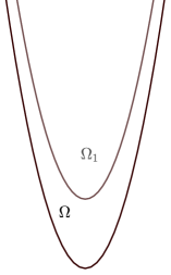
Recall that a convex set is strictly convex provided its boundary does not contain linear segments. Equivalently, a set is strictly convex if and only if any point of its boundary is an exposed point, i. e., it is the unique point of intersection of the boundary with a supporting hyperplane. The second assumption somehow says and behave in a similar way at infinity. It may be restated: and have congruent maximal inscribed cones; this assumption is meaningless if is bounded. The domains on Fig. 1 satisfy conditions (LABEL:StrictConvexity) and (2) because the corresponding domains defined in (2.1) do not contain infinite rays. The domain between two shifted hyperbolas (see Fig. 2),
| (2.15) |
contains infinite rays, e.g., the ones parallel to the coordinate axes. It still satisfies condition (2). The second domain on Fig. 2,
| (2.16) |
does not satisfy the cone condition.
The domains of this type (i. e., a set theoretic difference of two strictly convex sets, the smaller one lying strictly inside the larger one, and such that (2) holds true) will be informally called lenses. In the proof of the following lemma we will use the notation to denote the straight line segment that connects with .
Lemma 2.4.
Assume the domains and satisfy (LABEL:StrictConvexity). In the case we additionally assume (2). Then, for any there exists a segment passing through and whose endpoints lie on .

Proof.
Consider the case first. Let be the closest to point in , it is clear that . Let be a line passing through that is perpendicular to (if , we take to be a supporting line to at ). Note that does not intersect and separates from . By (LABEL:StrictConvexity), the intersection of any translate of with is bounded. Thus, by (2), the intersection of the translate of passing through with is a finite segment, let it be . It remains to note that .
Now let us turn to the case . We will argue by induction over dimension. In fact, it suffices to show that for any there exists an affine hyperplane passing through such that is bounded. If this assertion is proved, we may work inside the dimensional plane (condition (2) holds true for bounded domains). The desired hyperplane is also easy to find: pick any supporting hyperplane to and translate it to (the intersection of this translated supported hyperplane and is compact by (LABEL:StrictConvexity)). ∎
Remark 2.5.
In the assumptions of Lemma 2.4, if , then may be chosen in such a way that as well.
Corollary 2.6.
In the assumptions of Lemma 2.4, for any there exists such that .
Proof.
Construct a segment with the help of Lemma 2.4: there exist points and non-negative numbers and with sum one such that
| (2.17) |
Then, the desired function may be constructed as
| (2.18) |
here we set for convenience (all the considerations do not depend on the particular choice of ). By construction, for any , the point lies inside . Therefore, . ∎
3 Functionals
Let be a Borel measurable locally bounded function. We wish to find sharp estimates of the expression when . Note that a priori it is unclear whether the integral in question exists. The function
| (3.1) |
is well defined in the case where is bounded from below (though this function may attain the value ). The function
| (3.2) |
is a meaningful object for any locally bounded from below. Note that all the Bellman functions in the paper do not depend on the choice of , because the classes of functions (see (2.2)) and the Bellman functions themselves are defined in terms of averages. We will often omit the symbols and in the notation for our Bellman functions and simply write and . We also use the notation . Of course, we expect that the functions and coincide in reasonable situations. However, the proof of this assertion might be unexpectedly difficult.
Remark 3.1.
Now we pass to the examples and show how the Bellman functions above help to find sharp constants in various inequalities. We do not provide many details for the first two examples since they are discussed in the cited papers.
Muckenhoupt classes.
Scalar space.
Consider the domains (2.7) with . The choice leads to the sharp John–Nirenberg inequality in integral form, see [16]. The function was used to obtain sharp results on the constants in the inequalities that express the equivalence of different norms on , see [17]. For weak-type estimates, we may choose the function , see [22]. For quite general boundary values , the function (3.1) was computed in [10] (see a simpler version [9] and the short report [7]).
For larger similar Bellman functions will lead to sharp inequalities for vectorial functions.
Functions of bounded mean oscillation with values in the unit sphere.
A version of the John–Nirenberg inequality for functions between manifolds may be found in Appendix B of [3]. In that paper the inequality is stated in its integral form, here we prefer to work with the classical ’tail estimate’ form as in [11]. For that consider the class generated by the domains and given in (2.12). Pick some point and some . Consider the function
| (3.4) |
and the Bellman function (3.1) generated by this boundary value. The Bellman function delivers sharp estimate of the amount of points such that
| (3.5) |
provided belongs to the -ball of and . If we choose , we obtain the sharp estimate for the quantity
| (3.6) |
The John–Nirenberg inequality says this quantity decays exponentially as decreases down to zero. The Bellman function allows to find the sharp constants in the corresponding inequality, see the forthcoming paper [4].
Multiplicative inequalities.
Consider the domains given by (2.13) and the corresponding class . Let , where . The corresponding Bellman function delivers sharp upper estimates for the -norm of a function provided its average, -norm, and norms are fixed. This, in particular leads to computation of sharp constants in the multiplicative inequalities
| (3.7) |
4 Locally concave functions and martingales
Definition 4.1.
Let . We say that a function is locally concave provided its restriction to any segment is concave.
Here and in what follows we will be using the convention that concave functions may attain infinite values, see [14]. It is important that we do not allow the value (see a pathological example at the end of this section). Locally concave functions play important role in the Bellman function theory; see [5] for applications to geometry. In the definition below, is the set of all points such that there does not exist a segment with lying in the interior of ; the latter set is called the fixed boundary (because we fix the boundary values of locally concave functions on this set). The remaining part of the boundary is called the free boundary and is denoted by . In our usual examples of a lens , we have and . From now on we will be using this notation.
Definition 4.2.
Let , let be a function. By we denote the class of all locally concave on functions that satisfy the boundary inequality for any .
Remark 4.3.
By Theorem in [14], any function is continuous on the interior of as a mapping with values in .
We are ready to define the pointwise minimal locally concave function
| (4.1) |
(note that if this function does not attain the value ) and state our first main theorem. The notation means that locally coincides with a graph of a -smooth function. Recall .
Theorem 4.4.
Let the domains and satisfy the usual requirements , (LABEL:StrictConvexity), (2), and let also . Let the function be lower semi-continuous and bounded from below. Then,
| (4.2) |
This theorem generalizes, up to minor modifications, the main result of [21]; in that paper we had and unbounded (and, therefore, unbounded ). The methods of [21] relied upon the notion of monotonic (non-decreasing) rearrangement, which, seemingly, does not exist in the case where is not simply connected. A good replacement for monotonic rearrangements was found in [20]. The disadvantage of this new method is that it does not allow to work with . The main theorem in [21] states identity (4.2) for all . Seemingly, in the larger generality Theorem 4.4 is also true for , however, the methods from [20] do not allow to prove it (see Section 9 below for an explanation).
We need to survey the notions from [21] we will be using. We will be working with discrete time martingales adapted to a filtration . We refer the reader to [15] for the general martingale theory and present here the simplified definitions we will use.
By a filtration we mean a sequence of increasing set algebras (we consider finite algebras only), that is if , then as well. A sequence of random variables taking values in some linear space is called a martingale adapted to provided, first, each is -measurable, and second, for each we have . Note that since our algebras are simple, we may freely work in infinite dimensional spaces (in the case of general martingales, there are difficulties with the definition of conditional expectation, see Section in [6]). All martingales we will be working with have the limit value , a random variable that generates the martingale:
| (4.3) |
Here we should take care, should attain values in a finite dimensional space since we wish to omit the theory of integration of functions taking values in infinite-dimensional spaces.
The main property of may be restated: for any atom (by an atom of a set algebra we mean a set of positive measure that is minimal by inclusion), one may restore the value of on this atom by the formula
| (4.4) |
We cite an important definition from [21]. See Fig. 4 for an example.
Definition 4.5.
Let . An -valued martingale adapted to is called an -martingale, provided
-
1)
the algebra is trivial, i. e., consists of the whole probability space and the empty set;
-
2)
there exists a random variable with the values in such that in and almost everywhere (in particular, is summable itself);
-
3)
for any atom there exists a convex set such that lies in almost surely.
Sometimes, we will need to use a slightly modified notion of an -martingale introduced in [20].
Definition 4.6.
Let and let . An -martingale is called an -martingale, provided almost surely.
Remark 4.7.
We may also consider or -martingales for infinite-dimensional domains . However, in this case we require that attains values in the intersection of with a finite dimensional space. For example, this happens if attains finitely many values.


Consider two other Bellman functions on : the first one is defined for measurable and bounded from below,
| (4.5) |
and the second one is defined for arbitrary locally bounded from below measurable :
| (4.6) |
Recall that a martingale is called simple if there exists a natural number such that for all . We will use Theorem from [21]. It uses the notion of a strongly martingale connected domain. A set is called strongly martingale connected if for every there exists a simple -martingale that starts at , that is .
Lemma 4.8.
Assume (LABEL:StrictConvexity). The domains and are strongly martingale connected if either or (2) holds true.
Proof.
Consider the case of the domain first. Let , we wish to construct a simple -martingale starting at . If , then the desired martingale is constantly equal . So, we may assume . By Lemma 2.4, there exists a segment with the endpoints and lying on , passing through . In other words,
| (4.7) |
Let us construct the martingale by the formula,
| (4.8) |
In other words, is a martingale that starts at , splits into and , and stops there. Since , is the desired simple -martingale.
Theorem 4.9 (Theorem in [21]).
Let be a strongly martingale connected domain. Let be a bounded from below function such that is continuous at every point of the fixed boundary. Then, for all .
Remark of the same paper says that if is only locally bounded from below, is continuous at the points of the fixed boundary, then . We will need a slightly stronger statement. Let us introduce yet another Bellman function
| (4.9) |
Clearly, . We claim that this chain of inequalities often turns into a chain of equalities.
Lemma 4.10.
Let be a strongly martingale connected domain. Let be any measurable function. Then, for any .
Proof.
The proof is a simplification of the proof of Theorem in [21]; we provide a comment about simplifications. It suffices to prove the inequalities and for any .
To show the first inequality, it suffices to check the inclusion and use the definition of . It is clear that satisfies the boundary condition. By the requirement that is strongly martingale connected, does not attain the value . The local concavity may be verified similar to the proof of Lemma in [21].
To show the reverse inequality , it suffices to prove that for any simple -martingale with and any , the inequality
| (4.10) |
holds true. This inequality follows from Lemma in [21] that says that the quantity is non-increasing in this case; note that the assumption that is simple cancels the need for the limit argument (compare with the proof of Lemma 2.19 in [21]). ∎
A simple modification of the proof above allows to prove a version of Theorem 4.9.
Theorem 4.11.
Let be a strongly martingale connected domain. Let be a bounded from below function such that is lower semi-continuous at every point of the fixed boundary. Then, for all .
We will also need a technical statement in the spirit of Proposition in [21]. The proof is also very similar, so, we omit it.
Proposition 4.12.
Let , let . Suppose there exists a closed ball such that is a closed strictly convex set. Suppose nowhere equals . Then, is lower semi-continuous at the point provided is.
Surprisingly, the assertion of Lemma 4.10 becomes false without the assumption is strongly martingale connected. We use a little bit of complex variable notation to indicate points in the plane. Let be given by the rule
| (4.11) |

The main feature of the specific numbers in (4.11) is that the three small circles almost touch (see Fig. 5). By definition, . Let on the fixed boundary. In this case,
On the other hand, Lemma in [21] says (the domain is a cheese domain in the terminology of that paper). Therefore, and does not coincide with . The effect of similar nature arises when one defines rank-one or separate convex hulls, see [12].
5 Functions on the circle and the line
During the proof, we will need to work with functions defined on the circle of unit length (in other words, its radius equals ). Let us equip with the natural arc length measure. We will think of functions on as of periodic functions on the line, i. e., identify the function with its periodic version , here
| (5.1) |
Consider a version of the class (2.2) formed from summable -valued functions on :
| (5.2) |
Note that in this definition we require the ’boundedness of oscillation’ over arcs that may wind around the circle several times. The additional domain is mostly needed for technical purposes, it seems to be unavoidable in Lemma 6.1 below.
Remark 5.1.
Recall .
Lemma 5.2.
Assume the domains satisfy (LABEL:StrictConvexity). In the case we additionally assume (2). For any there exists such that .
Proof.
Consider the Bellman functions
| (5.3) |
and
| (5.4) |
Similar to (3.1) and (3.2), we define the function (5.3) for that is bounded from below, whereas the function is a meaningful object for any locally bounded from below. Since for any , we have
| (5.5) |
The theorem below is our second main result.
Theorem 5.3.
Let the domains and satisfy the usual requirements , (LABEL:StrictConvexity), and (2). Let the function be lower semi-continuous and bounded from below. Then,
| (5.6) |
Proposition 5.4.
Let the domains and satisfy the requirements and (LABEL:StrictConvexity). Let the function be locally bounded. Then,
| (5.7) |
Before we pass to the proofs, we need to survey the theory from [20].
Definition 5.5.
We say that two -valued random variables and are equidistributed provided they have the same distributions, which means
| (5.8) |
for any measurable set .
Note that if and are equidistributed, then for any function such that one of these mathematical expectations exists. If and is an interval, then by we denote the distribution of the random variable . In other words,
| (5.9) |
Note that is a probability measure on . Consider the set of all probability measures on with bounded first moment. The set is a convex subset of the space of all finite signed measures on with bounded first moment. Let be a subset of . We will always impose two conditions on this set:
| (5.10) | ||||
| is open in the topology of the latter space. |
Note that . We will be working with simple martingales that attain their values in the space ; these martingales are easy to define since a simple martingale attains values in a finite dimensional linear space. We denote by the distribution of the function itself, i. e., .
Theorem 5.6 (Theorem in [20] with slight modifications).
The theorem above will serve as a tool to construct functions with prescribed distributions. We must say about the difference between the formulations above and in [20]. We require weaker openness condition on here, in [20] the set was open in weak-* topology. One may go through the proof in [20] and realize that everything happens in the finite dimensional space spanned by the values of . We will apply the theorem to the sets
| (5.11) |
Note that the intersection of with any finite dimensional space spanned by delta measures is open. By definition, the condition is almost equivalent to the condition that for any subinterval (the word ‘almost’ corresponds to the presence of the set in (5.2)). We will later show that any simple -martingale generates a simple martingale with values in that satisfies the conditions of Theorem 5.6 with given in (5.11). This observation will allow us to construct a function that has the same distribution as (see Lemma 6.2 below).
6 Proof of Theorem 5.3
The proof will be based on two lemmas below.
Lemma 6.1 (Splitting lemma).
Assume satisfies (LABEL:StrictConvexity) and (2). Let and let be an open set such that , let . There exists an -martingale such that is equidistributed with .
We will call the domain as in lemma above an extension of .
Lemma 6.2 (Gluing lemma).
Assume satisfies (LABEL:StrictConvexity) and (2). Let be a simple -martingale. There exists a function that is equidistributed with .
Proof of Theorem 5.3..
It suffices to prove the inequalities
| (6.1) | |||
Without loss of generality assume that is finite. Let us first prove (LABEL:CircleThFirstIneq). Fix . By (5.3), for any there exists such that
| (6.2) |
Let be the set that corresponds to in (5.2). By Remark 5.1 we assume is strictly convex and satisfies (LABEL:StrictConvexity) and (2). Then, is an extension of . We apply Lemma 6.1 to the function with in the role of extension of and obtain an -martingale such that is equidistributed with . Then,
| (6.3) |
the last inequality follows from Theorem 4.11, Proposition 4.12, and Lemma 4.8. It remains to choose arbitrarily small .
The proof of Lemma 6.1 follows the lines of the proof of Theorem in [21]. We introduce the function :
| (6.6) |
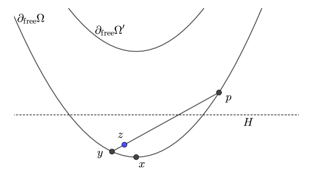
We will also often use the notion of a transversal segment. See Fig. 6 for visualization.

Definition 6.3.
Let , let be a segment with the endpoint . We say that is transversal provided the line containing it intersects .
Lemma 6.4.
Let and satisfy (LABEL:StrictConvexity). Let be such that . Then, the condition (2) is equivalent to the fact that for any choice of the function is uniformly bounded on any compact subset of .
Proof.
Let us first verify the necessity of (2). Assume it does not hold and there exists a ray such that it cannot be shifted inside . Without loss of generality, we may assume starts from and does not intersect . By (LABEL:StrictConvexity), we may also assume is a transversal segment. Let us choose in such a manner that it intersects the continuation of beyond , let belong to that intersection. Choosing as far as we wish on , we obtain that the ratio , and thus, the value , is unbounded.
Now we turn to the sufficiency of (2). Let be a compact set. First, we note that
| (6.7) |
Second, it suffices to prove that the quantity is uniformly bounded whenever , , and there exists such that . Assume the contrary. Let there exist sequences , , and such that
| (6.8) |
Without loss of generality, we may assume that and , where . By the closedness of , the ray lies inside entirely. By (LABEL:StrictConvexity), does not contain lines, so is uniformly bounded. We may assume . This means cannot be shifted to lie inside , which contradicts (2). ∎
Proof of Lemma 6.1..
Given a function , there exists a partition , with being disjoint (up to a common point) intervals such that
| (6.9) |
The proof of this statement is completely similar to the proof of Lemma in [21]. We apply it inductively to build a sequence of partitions of such that
-
1)
for each the partition is a subpartition of , moreover, for each and , , one has ;
-
2)
for each and , , the segment lies in ;
-
3)
for each and , , .
Let be generated by , let . The martingale is the desired -martingale (the proof of this assertion is identical to the proof of Theorem in [21]). ∎
Remark 6.5.
The assertion of Lemma 6.1 remains true if does not necessarily satisfy (2), however, . The proof should be modified as follows. We choose a compact convex set such that almost surely. We consider the function
| (6.10) |
This function is bounded since is separated away from zero and is bounded. Now we may repeat the proof of Lemma 6.1 with in the role of .
Proof of Lemma 6.2..
Let be a simple martingale. Note that we may choose the sets in Definition 4.5 to be closed simplices. Let be the union of such simplices over all atoms of all algebras . In fact, this is union of a finite number of simplices. Thus, is a compact subset of . Therefore, is separated from and does not intersect with the sets for sufficiently close to , here
| (6.11) |
we use the standard Minkowski addition. Fix some close to such that and set . Note that the corresponding lens satisfies (LABEL:StrictConvexity) and (2)111Alternatively, the set may be constructed with the help of Theorem 8.17 below.. What is more, . Thus, fits into formula (5.2) and is an -martingale. Consider the set
| (6.12) |
This set satisfies the two requirements on the set listed in (5.10). It is high time to make our choice for the martingale . Recall the martingale is simple. The desired martingale is defined by the formula
| (6.13) |
here denotes the distribution of the random variable ; we treat as a random variable on the probability space equipped with the measure . Let us prove that is an -martingale with given in (6.12). We will firstly show that is indeed a martingale. For that we choose an arbitrary and an atom . Let be the kids of . The martingale property of is
| (6.14) |
To prove this identity in measures, we may test it against a Borel set :
| (6.15) |
which is true. It remains to verify the third property in Definition 4.5. We need to check that any convex combination lies inside the set . This means
| (6.16) |
This reduces to the fact that is an -martingale since
| (6.17) |
We apply Theorem 5.6 to and and obtain a function with . It remains to notice that is the distribution of . ∎
7 Proof of Proposition 5.4
First, the inequality
| (7.1) |
follows from (4.1) since whenever , its restriction to belongs to . Second, to prove the reverse inequality to (7.1), it suffices to construct a function such that
| (7.2) |
The construction of the function is fairly straightforward, however, the verification of its local concavity will take some time. To construct , we will use special segments . For any let us choose some transversal (see Def. 6.3) segment with the endpoint . Define the function by the formula
| (7.3) |
where approaches along . Note that the limit in the formula always exists (though it might be equal to ) since is a concave function.
Lemma 7.1.
Let satisfy (LABEL:StrictConvexity), let . Let be a transversal segment with the endpoint . Let be another segment with the endpoint . Then, the convex hull of and also belongs to entirely.
Proof.
It suffices to prove that the said convex hull is disjoint with . Assume the contrary, let lie in the convex hull of and . Let be a point on the continuation of over the point that is sufficiently close to . Since is a transversal segment, . The segment then lies inside since is convex. On the other hand, , clearly, intersects , which contradicts . ∎
Remark 7.2.
In fact, the said convex hull lies inside except for the point itself.
Proof of Proposition 5.4.
As we have said, it suffices to show given in (7.3) is locally concave on (in particular, we need to verify that does not attain the value ). The verification of local concavity consists of checking the inequalities
| (7.4) |
We are interested in the cases where one of the points , or lies on . Let be distinct points.
Case .
Note that in this case and do not lie on by (LABEL:StrictConvexity). Thus, we may assume they are interior points of . Consider the segment , some point (let ), and the points , , and given by the rule
| (7.5) |
here stands either for , or for , or for . Note that by Lemma 7.1 (with Remark 7.2). Thus,
| (7.6) |
Note that as . Thus, (7.4) is proved in this case since is continuous at and .
The reasoning above also shows that . Indeed, we need to choose some points such that and use (7.4).
Case .
Consider the segment . Let . We consider the points , , and defined by the same formula (7.5). By Lemma 7.1 (Remark 7.2), these points lie inside together with the segment . Thus, (7.6) holds true and (7.4) follows by a limit argument. ∎
Remark 7.3.
One may prove that the definition of the function by (7.3) does not depend on the particular choice of transversal segments .
8 Proof of Theorem 4.4
Theorem 4.4 immediately follows from (5.5), Theorem 5.3, and Proposition 5.4 once we prove the ’extension’ theorem below.
Theorem 8.1.
Let be a lens that satisfies (LABEL:StrictConvexity) and (2). Assume is -smooth and is an arbitrary function. Then,
| (8.1) |
When proving Theorem 8.1, we may assume, without loss of generality, that is finite. Then, the identity (8.1) may be reformulated: for any and any there exists an extension such that
| (8.2) |
Note that may depend on and . In the case of smooth boundaries and sufficiently regular , we will prove a stronger statement, which is the main step toward the proof of Theorem 8.1.
Theorem 8.2.
Let be a lens that satisfies (LABEL:StrictConvexity) and (2). Assume the boundaries are -smooth and the function is -smooth as well. Then, for any there exists an extension such that
| (8.3) |
for any .
The proof of this theorem follows the proof of Theorem in [21] with some modifications. These modifications do not require new ideas, however, some re-phrasing is needed to work in with arbitrary instead of . The condition may be immediately replaced with being merely continuous by approximation in the uniform norm. Here we have used the obvious inequalities
provided .
Corollary 8.3.
The statement of Theorem 8.2 holds true if .
The method of [21] was to perturb the function a little bit to make it strongly concave and then to extend it through the free boundary. The reasoning naturally splits into two steps: first, we study the boundary behavior of minimal locally concave functions and, second, use this structure to construct the extension.
8.1 Boundary behavior of minimal locally concave functions
Definition 8.4.
Let . We say that two points see each other if . The set
| (8.4) |
is called the set of points visible from .
We will simply write instead of when the ambient set is clear from the context.
Proposition 8.5.
Let be a lens that satisfies (LABEL:StrictConvexity) and (2). The set is compact whenever . The diameter of is uniformly bounded when runs through a compact subset of .
Proof.
It is clear that the set is closed (since is closed). So we only need to prove the second assertion. Assume the contrary, let there exist a sequence with values in a compact subset of and a sequence such that and . Without loss of generality, and . Then, by the closedness of , the ray lies inside . By (2), there exists such that . This contradicts the strict convexity of since . ∎
Remark 8.6.
The set is not necessarily bounded if as the left picture on Figure 2 shows.
We will often use the following simple principle (compare with Fact in [21]).
Fact 8.7.
Let be a strictly convex subset of . Suppose that there are positive and and a point such that , . Then for and any one may find such that .
For the hint to the proof see Figure 7.

Definition 8.8.
Let and let . The set of linear functions such that holds for any is called the superdifferential of at . We will denote it by .
Fact 8.9.
Let and let . Assume for every the superdifferential of at is non-empty. Then, the function is locally concave on .
Every concave function has a non-empty superdifferetial at interior points of its domain (see, e. g., Section in [14]). One may ask whether the superdifferential is non-empty for every in provided is locally concave. The answer to this question is negative in general (consider the domain formed by three lines passing through the origin in ). However, for some good domains (lenses among them) and sufficiently good functions, the answer is positive.
Proposition 8.10.
Let be a lens that satisfies (LABEL:StrictConvexity) and (2). Assume that the boundaries of are -smooth. Let be a locally Lipschitz function such that is finite. For any there exists a linear function such that
| (8.5) |
for all . In other words, is non-empty.
Remark 8.11.
One may replace the minimal locally concave function with an arbitrary locally concave function provided is locally Lipschitz.
Proof.
Without loss of generality, we may assume and
| (8.6) |
The symbol denotes the tangent plane to at the point . We also assume on . By concavity of , there exists a linear function such that
| (8.7) |
for any satisfying . Let denote the orthogonal projection onto . Let
| (8.8) |
We claim that
| (8.11) |
Indeed, (8.11) clearly does not exceed (8.8). On the other hand, if
| (8.12) |
for all and some , then the same inequality holds true for all by minimality of . Indeed, if this is not the case, the function
| (8.13) |
lies in and is smaller than , which is a contradiction. Thus, the two supremums on the right hand sides of (8.8) and (8.11) coincide.
Now let us prove that the local Lipschitz property of implies is a finite quantity. Let be a sequence of points in that realizes the supremum in (8.11). Assume . If , then is finite.
Remark 8.12.
It follows from construction that the coefficients of the linear function are uniformly bounded when runs through a compact subset of .
Proposition 8.13.
Let be a lens that satisfies (LABEL:StrictConvexity) and (2). Assume that the boundaries of are -smooth. Let be a -smooth function such that is finite. Let be the linear functions constructed by formulas (8.11) and (8.16), here . Then, there exists a point such that
| (8.17) |
The constant in this inequality is uniform when runs through a compact set on .
Proof.
Let be a limit point of the sequence that realizes the supremum in (8.11). We will show that the choice with fulfills (8.17). Let us first prove . If , then this follows from the definition of . In the case , we have ; if this identity does not hold, the supremum equals , which is definitely false. Therefore, .
Let us consider the -smoth function
| (8.19) |
We have . If , then is non-positive in a neighborhood of . Therefore, is a local maximum of , and (8.17) follows.
If , then we know that for such that . From (8.11) we know that for any we have for sufficiently large . Let us consider the hyperplane that contains the intersection and is parallel to the -axis. Without loss of generality, we may assume this hyperplane is . Let be the projection of onto this plane defined near : if is the orthogonal projection, then
| (8.20) |
The function is -smooth in a neighborhood of , , and when . What is more, there is a sequence such that , , and
| (8.21) |
for any fixed provided is sufficiently large.
Let us prove that . The restriction of to the section attains its maximum at , therefore, we only need to check that
| (8.22) |
Note that the derivative on the left hand side cannot be negative since when . Let us prove it is non-positive. If this is not the case, then for some , and, by -continuity, it follows that in a neighborhood of . Then,
| (8.23) |
which contradicts (8.21). Therefore, . Then, for any sufficiently close to we have
| (8.24) |
which proves (8.17). ∎
Remark 8.14.
The condition is superfluous. One may replace it with as it can be seen from the proof.
Proposition 8.15.
Let be a lens that satisfies (LABEL:StrictConvexity) and (2). Assume that the boundaries of are -smooth. Let be a -smooth function such that is finite. Let be the linear functions constructed by formulas (8.11) and (8.16), here . Then,
| (8.25) |
The implicit constants hidden by the -notation are uniform when and run through a compact set on .
Proof.
By compactness argument, it suffices to consider the case where lies in a neighborhood of . Similar to the proof of Proposition 8.10, we assume ,
| (8.26) |
and on . Let be defined as the graph of the function , where is a neighborhood of the origin. Consider the cone
| (8.27) |
where is a point in a neighborhood of and is a sufficiently large constant. See Fig. 8 for visualization.


The cone does not intersect .
Let us prove this claim. Since the tangent plane to at the point is described by the equation , it suffices to prove the inequality
| (8.28) |
We estimate
| (8.29) |
The inequality for all in a compact set and all in a neighborhood of follows from the -smoothness assumption about . Thus, indeed does not intersect .
A similar reasoning shows that
| (8.30) |
In particular, in such a case cannot belong to .
Let be the point constructed in Proposition 8.13. We consider two cases: and .
Case .
In this case, and the segment intersects (since lies below the plane by (8.30)). Denote the point of intersection by . Then, the function defined by
| (8.31) |
is concave on this segment, attains the value at and is non-positive at . Thus, it is non-positive at as well, and we have proved , which is stronger than (8.25).
Consider the case .
There exists a point such that . For example, such a point can be found in the two-dimensional plane that passes through , , and is orthogonal to the plane (here we use Proposition 8.5; see also the second drawing on Fig. 8). The segment intersects the plane at the point . By (8.30),
| (8.32) |
Corollary 8.16.
Let be a lens that satisfies (LABEL:StrictConvexity) and (2). Assume that the boundaries of are -smooth. Let be a -smooth function such that is finite. For any there exists a function that is locally concave on and satisfies the inequalities
| (8.35) |
moreover, for any there exists a linear function such that for any compact set the inequality
| (8.36) |
holds true with the positive constants and depending on only. The coefficients of the linear functions are uniformly bounded when runs through a compact subset of .
Proof.
8.2 Construction of the extension
Before we pass to the details, we will survey our method for construction of extensions. Assume is a locally concave function on some set and assume its superdifferential is non-empty at each point . Let be a set such that . Then, we can extend to by the formula
| (8.39) |
The formula is not completely rigorous, because sometimes it is convenient to take all linear functions from the superdifferential of at , sometimes we may pick only one. There are two questions concerning formula (8.39): when do we obtain a finite function and when is it locally concave on ? We will give two simple sufficient conditions.
The function is finite when all are uniformly bounded when runs through a compact set and for any , the set is compact.
The function is locally concave provided for any there exists a neighborhood (in the relative topology of ) and a point such that for any and
| (8.40) |
Then and the local concavity follows from Fact 8.9.
We will also need two theorems about approximation. For more details and proofs, see [2] (based on earlier work in [1]).
Theorem 8.17.
Let be a non-empty strictly convex open proper subset of . Let be an open set that contains . There exists another open set such that , , and is a strictly convex set with real-analytic boundary.
Theorem 8.18.
Let be a non-empty strictly convex open proper subset of . Let be a closed set that lies inside . There exists another open set such that and is a strictly convex set with real-analytic boundary.
Proposition 8.19.
Let be a non-empty strictly convex open proper subset of . Let be a continuous function. There exists a strictly convex open set with real-analytic boundary such that and if see each other in then .
Proof.
Consider the set
| (8.41) |
This set is closed and lies inside . If two points see each other in , then . It remains to apply Theorem 8.18 to replace with a larger set . ∎
Corollary 8.20.
Let be a lens that satisfies (LABEL:StrictConvexity) and (2). Assume that the boundaries of are -smooth. Let be a -smooth function such that is finite. For any there exists an extension whose boundaries are -smooth and a function that is locally concave on and satisfies the inequalities
| (8.42) |
moreover, for any there exists a linear function such that for any compact set there exists such that (8.36) holds true whenever see each other in . The coefficients of the linear functions are uniformly bounded when runs through a compact subset of .
Now we are ready to define our extension by a formula similar to (8.39):
| (8.43) |
Lemma 8.21.
For any there exists a relatively open set that contains and such that for any the value is finite and the superdifferential of at is non-empty.
Proof.
Let be a hyperplane that separates from (say, is closer to than to the latter set). It suffices to prove that if is sufficiently close to , then the infimum in (8.43) is attained at that lies on the same side of as . See Fig. 9 for visualization. Then sees a neighborhood of and belongs to the superdifferential of at .
Let be a point that lies on the other side of than and that sees in . We wish to prove that there exists on the same side of as such that
| (8.44) |
provided is sufficiently close to . Let be the intersection of the line passing through and with lying on the same side of as . Let also be a compact set that contains with all the points it can see in and all the points the latter points can see. Let be the supremum of the Lipschitz constants of the functions when . Then,
| (8.47) |
We see that (8.44) indeed holds true provided is sufficiently close to , because in this case is also sufficiently close to while is bounded away from zero. ∎
Proof of Theorem 8.2..
8.3 Proof of Theorem 8.1
In order to prove Theorem 8.1, we will need to extend a locally convex function via formula (8.39) over the fixed boundary.
Lemma 8.22.
Let be a lens that satisfies the requirements (LABEL:StrictConvexity) and (2). Let be a set whose interior contains . Let be a locally Lipschitz function that is locally concave on and has non-empty superdifferential at each point. Assume is an open convex set that contains and such that each sees only a compact subset of in . Then, the function
| (8.49) |
is finite and locally concave on .
Proof.
By local concavity of , we may consider only when calculating the infimum in (8.49). Since the sets are compact and the function is locally Lipschitz on , does not attain the value . Thus, it remains to verify the local concavity of . For that, we will prove has a non-empty superdifferential at each point .
Let and assume , and . It suffices to prove when lies in a sufficiently small neighborhood of . This is true since sees in (now we are using the initial formula (8.49)). The reasoning in the case when the infimum that defines is attained at a sequence of does not differ. ∎
Fact 8.23.
Let be a strictly convex open set, let be a point of its boundary. There exists a neighborhood in such that any point can see only a compact subset of in .
Proof of Theorem 8.1.
Fix and .
First, we construct an open strictly convex set with real analytic boundary such that it contains the closure of and any point can see only a compact subset of in ; this is done by a combination of Theorem 8.17 and Fact 8.23.
Second, we construct a strictly convex set such that , , , and if and from see each other in , then ; this is done by application of Proposition 8.19 with , where is sufficiently small.
Note that any point can see only a compact subset of in . We also note that the restriction of the function to the set is locally Lipschitz and has a non-empty superdifferential at each point; the set is uniformly bounded for any compact set . Thus, we may construct the function by the formula
| (8.50) |
By Lemma 8.22, is a locally concave function. What is more, is continuous on . Therefore, the function
| (8.51) |
may be ’extended’ through the free boundary by Theorem 8.2. Let be the extension of , let be the ’extended’ function. Then,
| (8.52) |
∎
9 Limitations of current methods
The lemma below justifies the appearance of the auxiliary domain in (5.2). It also shows why we are not able to prove (4.2) for the points in Theorem 4.4. We recall the definition of a cheese domain from [21]. A set is called a cheese domain if it may be represented as
| (9.1) |
where the domains , are strictly convex, open, and bounded; the ‘holes’ , , are mutually separated and also lie inside the interior of .
Lemma 9.1.
Let be a cheese domain such that the domains in the representation (9.1) have -smooth boundaries. Let be such that for any arc the point lies in . If for some then attains two values.
Proof.
Without loss of generality, . Let be the tangent to at the point . We say that a point lies below if it is strictly separated by from and say that it lies above in the case the point and belong to the same open half-plane generated by .
We will first prove that does not attain values on the part of lying below . Assume the contrary. Let be a Lebesgue point of such that lies below . Consider the point
| (9.2) |
When is sufficiently close to , the point lies close to . Thus, the point (9.2) lies in a small neighborhood of and above . In particular, it does not belong to provided is sufficiently small. This is a contradiction.
Second, we will prove that does not attain values on the part of lying above . Consider an affine function that is equal to zero on and is negative below . Then, . On the other hand,
provided on a set of non-zero measure (since we have proved that is always non-negative). ∎
Finally we will show that the convexity of is necessary for (4.2) (note that the definition of the minimal locally concave function and the Bellman function do not require convexity of ).

We will shortly construct an example of and such that . Let be the unit circle. Consider three points
Define the function by the rule:
Fact 9.2.
The set of Bellman points of , i. e., the points , is
| (9.3) |
Now we construct the domain and the function . Define by the rule
We draw Figure 10 for reader’s convenience (the picture has slightly different numeric parameters, what is important is that the two ‘erased’ circles do not intersect the set (9.3), however, the average of lies above the lower common tangent to the circles).
Lemma 9.3.
Consider given by (9.4). Then, .
Proof.
It is clear that provided we extend the function to by the same formula (9.4). Consider the points and on the erased circles that have the smallest possible second coordinates. In other words, they are the points on the lower common tangent to these two circles. Similarly, let and be the points having the largest possible second coordinates.
Let be the linear function that coincides with on the segments and and let the part of lying between and be called the channel. Define the new function to be equal on the channel and to be equal everywhere else. It is easy to observe that is locally concave. On the other hand, and thus, . ∎
References
- [1] D. Azagra, Global and fine approximation of convex functions, Proc. Lond. Math. Soc. (3) 107 (2013), no. 4, 799–824.
- [2] D. Azagra and D. Stolyarov, Inner and outer smooth approximation of convex hypersurfaces. When is it possible?, https://arxiv.org/abs/2204.07498.
- [3] H. Brezis and L. Nirenberg, Degree theory and BMO. I. Compact manifolds without boundaries, Selecta Math. 1 (1995), no. 2, 197–263.
- [4] E. Dobronravov, On a minimal locally concave function on a ring, in preparation.
- [5] B. Guan, The Dirichlet problem for Monge-Ampère equations in non-convex domains and spacelike hypersurfaces of constant Gauss curvature, Trans. Amer. Math. Soc. 350 (1998), no. 12, 4955–4971.
- [6] T. Hytönen, J. van Neerven, M. Veraar, and L. Weis, Analysis in Banach spaces. Volume I: Martingales and Littlewood–Paley theory, Springer, 2016.
- [7] P. Ivanishvili, N. N. Osipov, D. M. Stolyarov, V. I. Vasyunin, and P. B. Zatitskiy, Sharp estimates of integral functionals on classes of functions with small mean oscillation, C. R. Math. Acad. Sci. Paris 350 (2012), no. 11, 561–564.
- [8] , On Bellman function for extremal problems in , C. R. Math. Acad. Sci. Paris 353 (2015), no. 12, 1081–1085.
- [9] P. Ivanishvili, N. N. Osipov, D. M. Stolyarov, V. I. Vasyunin, and P. B. Zatitskiy, Bellman function for extremal problems in , Trans. Amer. Math. Soc. 368 (2016), 3415–3468.
- [10] P. Ivanishvili, D. M. Stolyarov, V. I. Vasyunin, and P. B. Zatitskiy, Bellman function for extremal problems on II: evolution, Mem. Amer. Math. Soc. 255 (2018), no. 1220.
- [11] F. John and L. Nirenberg, On functions of bounded mean oscillation, Comm. Pure Appl. Math. 14 (1961), 415–426.
- [12] B. Kirchheim, S. Müller, and V. Šverák, Studying nonlinear pde by geometry in matrix space, Geometric analysis and nonlinear partial differential equations, Springer, Berlin, 2003, pp. 347–395.
- [13] A. Reznikov, Sharp weak type estimates for weights in the class , Rev. Mat. Iberoam. 29 (2013), no. 2, 433–478.
- [14] R. T. Rockafellar, Convex analysis, Princeton Mathematical Series, No. 28, Princeton University Press, Princeton, N.J., 1970.
- [15] A. N. Shiryaev, Probability. 2, Graduate Texts in Mathematics, vol. 95, Springer, New York, 2019, Third edition of [ MR0737192], Translated from the 2007 fourth Russian edition by R. P. Boas and D. M. Chibisov.
- [16] L. Slavin and V. Vasyunin, Sharp results in the integral form John–Nirenberg inequality, Trans. Amer. Math. Soc. 363 (2011), no. 8, 4135–4169.
- [17] , Sharp estimates on , Indiana Univ. Math. J. 61 (2012), no. 3, 1051–1110.
- [18] E. M. Stein, Harmonic analysis: real-variable methods, orthogonality, and oscillatory integrals, Princeton University Press, 1993.
- [19] D. Stolyarov, V. Vasyunin, and P. Zatitskiy, Sharp multiplicative inequalities with BMO I, J. Math. Anal. Appl. 492 (2020), no. 2, 124479, 17.
- [20] D. Stolyarov and P. Zatitskiy, Sharp transference principle for BMO and , J. Funct. Anal. 281, no. 6, 109085.
- [21] D. M. Stolyarov and P. B. Zatitskiy, Theory of locally concave functions and its applications to sharp estimates of integral functionals, Adv. Math. 291 (2016), 228–273.
- [22] V. Vasyunin and A. Volberg, Sharp constants in the classical weak form of the John–Nirenberg inequality, Proc. Lond. Math. Soc. 108 (2014), no. 6, 1417–1434.
- [23] V. Vasyunin, P. Zatitskiy, and I. Zlotnikov, Sharp multiplicative inequalities with BMO II, https://arxiv.org/abs/2111.05565.
- [24] V. I. Vasyunin, The sharp constant in the John–Nirenberg inequality, PDMI preprints 20/2003, http://www.pdmi.ras.ru/preprint/2003/03-20.html.
- [25] , The exact constant in the inverse Hölder inequality for Muckenhoupt weights, Algebra i Analiz 15 (2003), no. 1, 73–117.
- [26] , Mutual estimates for -norms and the Bellman function, Zap. Nauchn. Sem. S.-Peterburg. Otdel. Mat. Inst. Steklov. (POMI) 355 (2008), no. Issledovaniya po Lineĭnym Operatoram i Teorii Funktsiĭ. 36, 81–138, 237–238.
Dmitriy Stolyarov, [email protected],
St. Petersburg State University, Department of Mathematics and Computer Science;
Pavel Zatitskiy, [email protected],
St. Petersburg State University, Department of Mathematics and Computer Science.