On Imitation Learning of Linear Control Policies:
Enforcing Stability and Robustness Constraints via LMI Conditions

The set of $n$-dimensional real vectors is denoted as $\mathbb{R}^{n}$. The set of $m\times n$ real matrices is denoted as $\mathbb{R}^{m\times n}$. The identity matrix is denoted as $I$. For brevity, repeated blocks in lower triangular parts of symmetric matrices are replaced by “$*$”. When a matrix $P$ is positive semidefinite (definite), we will use the notation $P\succeq 0$ ($P\succ 0$). The spectral radius of $A$ is denoted as $\rho(A)$. The space $l_{2}$ is the space of square summable sequences with norm $||x||_{2}=(\sum^{\infty}_{i}|x_{i}|^{2})^{\frac{1}{2}}$. The Frobenius norm of a matrix $A\in\mathbb{R}^{n\times m}$ is denoted as $||A||_{F}$.

One typical setting for IL is that we are given a control design problem whose objective function is hard to specify beforehand. The autonomous driving example mentioned in the introduction is exactly one such problem. Then we can try to remedy this cost function design issue by directly fitting a policy on expert demonstrations. The hope is that the fitted policy can mimic the behaviors of experts and hence perform well on the given control problem. Specifically, suppose a sequence of state/action pairs $\{x_{k},u_{k}\}_{k=0}^{N}$ has been demonstrated by the expert. Now we want to fit a function $u=K(x)$ from these observed demonstrations. Such a behavior cloning approach leads to the following finite-sum optimization problem:

where $l$ is some loss function measuring the empirical performance of the fitted policy on observed demonstrations, and $r$ is a regularization term introduced to prevent overfitting. In the above formulation, the policy is typically parameterized as a linear function or a neural network. The resulting optimization problem is unconstrained and can be efficiently solved by stochastic gradient descent (SGD) or other first-order methods. Such a formulation can be problematic and inefficient for control applications where closed-loop stability, robustness, and safety become important design concerns. For example, it may require a large number of demonstrations to ensure the solution of the unconstrained optimization problem (1) to be a stabilizing policy, causing serious concerns on the efficiency and safety of the IL framework. Hence, it is more natural to adopt the following constrained optimization formulation:

where the policy fitting is confined to a feasible set $\mathcal{K}$ which is specified to carry the information of potential stability/robustness/safety constraints on $K$. Such a constrained optimization formulation helps reduce sample complexity and improve system safety at the price of introducing more challenging computational tasks. In general, the set $\mathcal{K}$ is non-convex, and the constrained optimization problem (2) is more difficult to solve compared with its unconstrained counterpart (1). This motivates the study in this paper. Specifically, we will consider a simpler benchmark problem where the plant dynamics and the underlying expert policy are both assumed to be linear. We will discuss how to solve (2) with various stability and robustness constraints in this setting.

Now we confine the scope of our paper to linear policy fitting. Suppose we want to fit a policy for a linear system with state $x_{t}$ and action $u_{t}$. We assume that the ground truth expert policy is linear, i.e.

where $e_{t}$ is some zero mean noise. Notice that the appearance of $e_{t}$ is quite natural and intuitive since there will always be some noise in the human expert’s demonstrations¹¹1In other words, humans will not make identical actions even given the same state observation.. Based on these assumptions, it suffices to only consider linear state-feedback policy parameterized by a static gain matrix $K$. In general, it will be insufficient to use linear policy to model human experts’ behaviors. It is our hope that our study on the simplified linear generative model (3) can bring some insights for more realistic settings.

Suppose we have gathered the demonstrated state/action pairs $\{x_{k},u_{k}\}_{k=0}^{N}$ from the generative model (3). Here we use “k” as the subscript to imply that the demonstrations may not be generated by a single trajectory of the underlying dynamical system. Our goal is to learn $K^{*}$ from the demonstrations. We can adopt the loss function and the regularization term used in [7] to formulate the following optimization problem

Typically, we can just set $l(Kx_{k},u_{k})=||Kx_{k}-u_{k}||_{2}^{2}$ and $r(K)=||K||_{F}^{2}$. The feasible set $\mathcal{K}$ needs to be further specified. A naive option is to consider an unconstrained setting. However, prior knowledge of $K^{*}$ can be used to confine the policy search to a much smaller feasible set and improve the performance of IL with fewer demonstrations. For example, the Kalman constraint can be enforced if $K^{*}$ is known to be the solution for some LQR problem [7], and ADMM can be applied to solve the resulting constrained optimization problem efficiently [7]. The Kalman constraint approach can significantly improve the sample efficiency of IL when the ground truth policy $K^{*}$ happens to be the solution for some LQR problem. Of course, the assumption that $K^{*}$ satisfies the Kalman constraint can be too strong and introduce unnecessary biases into the policy search when $K^{*}$ is only sub-optimal in the LQR sense. For such scenarios, weaker constraints are preferred. In this paper, we are mainly interested in the following two types of constraints.

1. 1.

   Stability: Consider the following LTI system

   $\displaystyle x_{t+1}$

   $\displaystyle=Ax_{t}+Bu_{t}+w_{t}$

   (5)

   where $w_{t}$ is some stochastic process noise. Suppose $A\in\mathbb{R}^{n_{x}\times n_{x}}$, and $B\in\mathbb{R}^{n_{u},n_{u}}$. A useful prior assumption on $K^{*}$ is that such that it should at least stabilize the closed-loop dynamics. Therefore, to incorporate such prior knowledge, we can specify the feasibility set in (4) as follows

   $\displaystyle\mathcal{K}=\{K:\rho(A+BK)<1\}.$

   (6)

   The stability constraint $\rho(A+BK)<1$ is much weaker than the Kalman constraint and will not introduce much bias into the policy fitting process.

2. 2.

   $\mathcal{H}_{\infty}$-robustness: Sometimes we will have prior knowledge on how robust $K^{*}$ is with respect to the model uncertainty. For example, we may know $K^{*}$ can stabilize the system (5) robustly in the presence of uncertainty in $A$ and $B$. The following feedback interconnection model provides a general model for (5) subject to various types of uncertainties.

   $\displaystyle\begin{split}x_{t+1}&=Ax_{t}+Bu_{t}+w_{t}+B_{1}v_{t}\\ z_{t}&=C_{1}x_{t}+D_{12}u_{t}\\ v&=\Delta(z)\end{split}$

   (7)

   where the uncertainty is modeled by a bounded operator $\Delta$ which is causal and maps any $\ell_{2}$ sequence $\{z_{t}\}$ to another $\ell_{2}$ sequence $\{v_{t}\}$. The above model is general since $\Delta$ can be set up properly to model uncertainty, nonlinearity, and time delays²²2For example, when the state/input matrices are not exactly known, the model (5) may be modified as $x_{t+1}=(A+\Delta_{A})x_{t}+(B+\Delta_{B})u_{t}+w_{t}$, which is a special case of (7) with $B_{1}=I$ and $v_{t}=\Delta_{A}x_{t}+\Delta_{B}u_{t}$.. Based on the famous small gain theorem [17], the system (7) is robustly stable for any $\Delta$ satisfying $\|\Delta\|_{\ell_{2}\rightarrow\ell_{2}}\leq\frac{1}{\gamma}$ if we have $\rho(A+BK)<1$ and $||F(K)||_{\infty}<\gamma$ where $F(K)$ is an LTI system defined as

   $\displaystyle F(K)=\left(\begin{array}[]{c|c}A+BK&B_{1}\\ \hline\cr C_{1}+D_{12}K&0\\ \end{array}\right).$

   Notice $||F(K)||_{\infty}$ denotes the $\mathcal{H}_{\infty}$-norm of $F(K)$. Therefore, if we know that the ground truth expert policy $K^{*}$ achieves the $\gamma$-level robustness, i.e. $||F(K^{*})||_{\infty}<\gamma$, we can enforce such a constraint during the policy fitting process by specifying

   $\displaystyle\mathcal{K}=\{K:\rho(A+BK)<1\,\,,\,\,||F(K)||_{\infty}<\gamma\}.$

   (8)

It is worth mentioning that there exist many other types of stability and robustness constraints which can be posed to confine the policy search. For readability and clarity, our paper focuses on the above two commonly-used constraints.

The feasible set specified by (6) or (8) is not convex in $K$, causing trouble for the constrained policy optimization. Fortunately, these stability/robustness conditions can be convexified as LMIs if we change variables properly. Now we briefly review these LMI conditions below.

1. 1.

   Convex conditions for stabilization: Notice that $K$ stabilizes the system (5) if and only if there exists a symmetric positive definite matrix $P\in\mathbb{R}^{n_{x}\times n_{x}}$ such that $P-(A+BK)^{\intercal}P(A+BK)\succ 0$. This condition is bilinear in $P$ and $K$, leading to a non-convex control design condition. However, we can apply the Schur complement lemma to obtain the following intermediate matrix inequality.

   $\displaystyle\begin{bmatrix}P^{-1}&(A+BK)P^{-1}\\ *&P^{-1}\end{bmatrix}\succ 0,\quad P^{-1}\succ 0$

   Then we can change variables as $(Q,L)=(P^{-1},KP^{-1})$ and obtain the following LMI condition:

   $\displaystyle\begin{bmatrix}Q&AQ+BL\\ *&Q\end{bmatrix}\succ 0,\quad Q\succ 0$

   (9)

   The above reparameterization is well-known [18]. Now we have a convex set of $(Q,L)$ which can be used to extract stabilizing policies efficiently. Since there is a one-to-one correspondence between $(P,K)$ and $(Q,L)$, such a reparameterization does not introduce any conservatism.

2. 2.

   Convex conditions for $\mathcal{H}_{\infty}$-robustness: We can impose an LMI condition which is similar to  (9) to describe all $K$ lying in the set (8). Specifically, we can set $K=LQ^{-1}$ to satisfy $\rho(A+BK)<1$ and $||F(K)||_{\infty}<\gamma$ if there exists $Q\in\mathbb{R}^{n_{x}\times n_{x}}$ and $L\in\mathbb{R}^{n_{u}\times n_{x}}$ such that the following LMI is satisfied.

   $\displaystyle\begin{bmatrix}Q&AQ+BL&B_{1}&0\\ *&Q&0&QC_{1}^{\intercal}+L^{\intercal}D_{12}^{\intercal}\\ *&*&I&0\\ *&*&*&\gamma^{2}I\end{bmatrix}\succ 0,\,Q\succ 0.$

   (10)

   Again, the above condition is convex in $(Q,L)$ and can be useful for our constrained policy fitting problem. As $\gamma\rightarrow\infty$, the $\mathcal{H}_{\infty}$-robustness condition (10) reduces to (9). Therefore, the $\mathcal{H}_{\infty}$-robustness assumption is a stronger prior which may be useful when $K^{*}$ happens to be robust. However, it may introduce some bias into policy fitting if $K^{*}$ is not robust in the first place.

From the above discussions, it becomes obvious that we can change the variable in the constrained policy fitting problem (4) to obtain a problem with a convex constraint. Notice such a parameterization method has been used in safe reinforcement learning [19]. Here we use it in the IL setting. To summarize, the constrained IL problem can be recast into the following general form:

where $\text{LMI}(Q,L)$ is some LMI with decision variables $(Q,L)$. If the only prior assumption is that the expert’s policy stabilizes the closed-loop dynamics, the stability constraint (9) will be used. If we further believe that the expert has achieved some level of robustness, the $\mathcal{H}_{\infty}$-robustness constraint (10) can be applied with some tuned $\gamma$. Although the objective function in (11) is non-convex, the constraint $\text{LMI}(Q,L)$ is convex and can be easily handled using projected gradient methods.

Although the objective function in (11) is non-convex, the projection onto the feasible set of the decision variables $(Q,L)$ is easy to compute. Therefore, simple optimization methods such as the projected gradient method or projected SGD can be readily applied. The projection step can be performed by solving the following convex subproblem.

Now we are ready to present our main algorithm which can be used to efficiently solve the constrained IL problem (11). The method that we use is the projected gradient descent (PGD) method, which is summarized as follows.

The matrices $(Q,L)$ are initialized by first finding a feasible solution of $\text{LMI}(Q,L)$. The gradient update performed on the objective in (11) is performed with a first-order batch method such as SGD [22]. If the number of samples is small (i.e. less than $\approx 50$), we compute the gradient with a single batch which reduces to regular gradient descent. The gradient can be calculated using any auto-differentiation method. In the next section, we will choose to use PyTorch due to its efficient implementation of batch operations in conjunction with auto-differentiation. The convex projection problem (12) and the feasibility of all LMIs can be solved using the CVXPY modeling framework [23] and the MOSEK solver [24].

By introducing the equality constraint $L=KQ$, we can obtain another useful equivalent form for (4) as follows

The decision variables for the above optimization problem are $(K,Q,L)$. Notice that (13) has a convex objective in $K$, a bilinear equality constraint in $(K,Q,L)$, and a convex inequality constraint in $(Q,L)$. This special structure allows us to apply ADMM just as in [7]. Denote $C(K)=\frac{1}{N}\sum^{N}_{k=0}l(Kx_{k},u_{k})+r(K)$. Then the augmented Lagrangian is given as $\mathcal{L}_{\rho}(K,Q,L,Y)=C(K)+\text{Tr}(Y^{\intercal}(KQ-L))+\frac{\rho}{2}||KQ-L||_{F}^{2}$, where $Y$ is the dual variable corresponding to the constraint $KQ=L$ and $\rho$ is a fixed scalar penalty parameter which must be sufficiently large to yield convergence [25] (we typically set $\rho=1$). Given initial parameters $(Q^{(0)},L^{(0)},Y^{(0)})$, the updates of ADMM follow a three-step optimization procedure, where each step is a convex problem:
1. In the $K$-step, we update the variable $K$ as

2. In the $(Q,L)$-step, we update $(Q,L)$ by solving the following semidefinite program:

3. In the $Y$-step, we update the variable $Y$ as

We can run the algorithm for a fixed number of iterations. Since the subproblems in ADMM are all convex, only CVXPY will be needed in the implementations. Note that ADMM is not necessarily superior to PGD in all settings, as we will see in the numerical case studies.

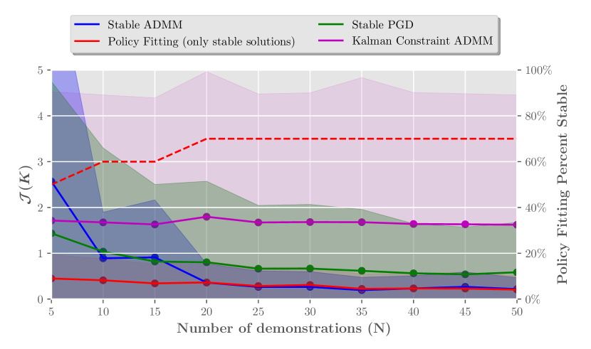
To evaluate the application of our approach for generally stabilizing policies that are not necessarily robust, we consider expert policies which are aggressive and not very robust (e.g. $A$ has eigenvalues which are close to $1$). Specifically, we generate $K^{*}$ by sampling uniform random initializations of $(Q,L)$ and then projecting via the LMI (9). Note that it is quite unlikely for the resultant matrix $K$ to be an optimal policy in either an LQR or $\mathcal{H}_{\infty}$ sense since any random initialization of $(Q,L)$ outside the stability feasible set will be projected to some interior point near the boundary of the feasible set. For each $K$, we measure how much the resulting state sequence $\{x_{i}\}_{i=1}^{N_{t}}$ under the closed-loop dynamics differs from the true closed-loop under $K^{*}$. Given the same initial condition, the cost is defined as $\mathcal{J}(K)=\frac{1}{N_{t}}\sum^{N_{t}}_{i=1}||x_{i}^{*}-x_{i}||_{2}^{2}$. In our simulations, the cost is averaged over $100$ random test trajectories of length $N_{t}=100$. This cost is chosen over the regular PF objective in (4) since it reflects the actual system behavior over time. To represent the performance of standard PF more fairly, we only average over stable solutions, while showing the percentage of stable solutions denoted by the red-dashed line in Figure 1. We show in Figure 1 that the standard PF problem (4) frequently produces unstable policies where the stability-constrained methods of PGD and ADMM maintain a low cost at all times. On the other hand, the Kalman constraint is biased towards LQR solutions with sufficient robustness margins, and hence a large gap persists between the stability constrained methods in this setting. We also note that there is a gap between PGD and ADMM, which may be due to the hyperparameters chosen in our simulations.

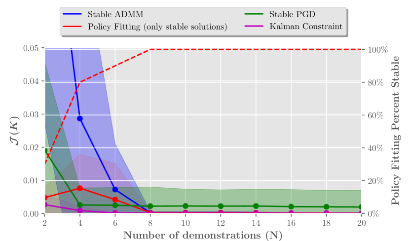
Next, we consider expert policies which are optimal with respect to the standard infinite horizon quadratic cost. For evaluation, a finite, yet large, horizon of ($N_{t}=1000$) is used to approximate the infinite horizon cost. We define the evaluation cost as $\mathcal{J}(K)=J^{(N_{t})}(K)-J^{(N_{t})}(K^{*})$. For illustrative purposes, we set $Q=R=I$. Since the optimal policy for an LQR problem has guaranteed stability margins, the expert policy $K^{*}$ is well within the feasible set and standard PF does not fail as often as in the previous aggressive case. While all constrained methods remain stable, it is hard to beat the inductive bias given by the Kalman constraint in the LQR setting. With enough data, our stable ADMM method approaches the performance of the Kalman constraint method. In this case, stable PGD performs better than ADMM in the lower data regime, while there is a small gap as $N$ grows, possibly due to the hyperparameter choices.

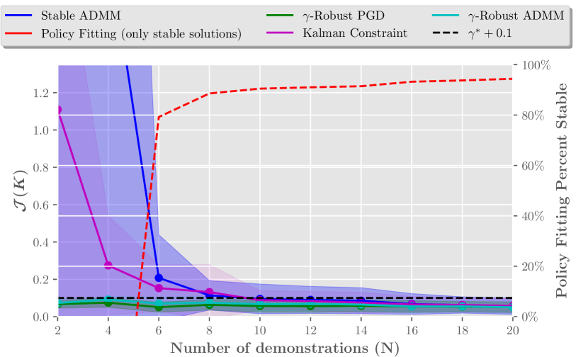
Lastly, we explore a useful application of the $\mathcal{H}_{\infty}$-robustness constraint (10) which ensures $||F(K)||_{\infty}<\gamma$ throughout the policy learning processes. For this experiment we choose $\gamma=\gamma^{*}+0.1$ where $\gamma^{*}$ is the optimal $H_{\infty}$ norm solution. Suppose we have prior knowledge of the robustness present in the system and choose $\gamma$ as an upper-bound estimate of the true $\mathcal{H}_{\infty}$ norm. In this case the demonstrator is a noisy $\mathcal{H}_{\infty}$ optimal controller for the sampled stabilizable system where $A_{ij},\,B_{1ij},B_{2ij}\sim\mathcal{\mathcal{U}}(-1,1)$, $C_{1}=I$, and $D_{12ij}\sim\mathcal{U}(-0.1,0.1)$. Here we have $B_{1}\in\mathbb{R}^{n_{x}\times n_{d}},D_{12}\in\mathbb{R}^{n_{z}\times n_{d}}$, $C_{1}\in\mathbb{R}^{n_{z},n_{x}}$ and $(n_{x},n_{u},n_{d},n_{z})=(4,2,1,4)$. The cost is given as $\mathcal{J}(K)=||F(K)||_{\infty}-||F(K^{*})||_{\infty}$. To study the effect of this additional $\mathcal{H}_{\infty}$-robustness constraint, we compare against the first proposed stability constraint (using ADMM), standard PF and the Kalman constraint method. We see that standard PF still produces some unstable solutions, but all the constrained IL methods eventually perform well. Stable ADMM and the Kalman constraint method produce stabilizing controllers through each trial, but with a much larger $\gamma$ initially. The Kalman constraint has inherent built-in margins which explains its performance over stable-ADMM when there are few demonstrations available. The robust ADMM and PGD methods produce an $\mathcal{H}_{\infty}$ norm much lower than other methods and stay within the prescribed $\gamma$ threshold for all trials.

References

- [1] B. D. Argall, S. Chernova, M. Veloso, and B. Browning, “A survey of robot learning from demonstration,” Robotics and autonomous systems, vol. 57, no. 5, pp. 469–483, 2009.
- [2] A. Hussein, M. M. Gaber, E. Elyan, and C. Jayne, “Imitation learning: A survey of learning methods,” ACM Computing Surveys (CSUR), vol. 50, no. 2, pp. 1–35, 2017.
- [3] T. Osa, J. Pajarinen, G. Neumann, J. A. Bagnell, P. Abbeel, J. Peters et al., “An algorithmic perspective on imitation learning,” Foundations and Trends® in Robotics, vol. 7, no. 1-2, pp. 1–179, 2018.
- [4] S. Ross, G. Gordon, and D. Bagnell, “A reduction of imitation learning and structured prediction to no-regret online learning,” in Proceedings of the fourteenth international conference on artificial intelligence and statistics, 2011, pp. 627–635.
- [5] J. Ho and S. Ermon, “Generative adversarial imitation learning,” in Advances in neural information processing systems, 2016, pp. 4565–4573.
- [6] K. Zhou and J. C. Doyle, Essentials of robust control. Prentice hall Upper Saddle River, NJ, 1998, vol. 104.
- [7] M. Palan, S. Barratt, A. McCauley, D. Sadigh, V. Sindhwani, and S. Boyd, “Fitting a linear control policy to demonstrations with a Kalman constraint,” ser. Proceedings of Machine Learning Research, vol. 120, 10–11 Jun 2020, pp. 374–383.
- [8] H. Yin, P. Seiler, M. Jin, and M. Arcak, “Imitation learning with stability and safety guarantees,” arXiv preprint arXiv:2012.09293, 2020.
- [9] S. Tu, A. Robey, and N. Matni, “Closing the closed-loop distribution shift in safe imitation learning,” arXiv preprint arXiv:2102.09161, 2021.
- [10] H.-N. Wu and B. Luo, “Simultaneous policy update algorithms for learning the solution of linear continuous-time state feedback control,” Information Sciences, vol. 222, pp. 472–485, 2013.
- [11] B. Luo, H.-N. Wu, and T. Huang, “Off-policy reinforcement learning for control design,” IEEE transactions on cybernetics, vol. 45, no. 1, pp. 65–76, 2014.
- [12] M. Han, Y. Tian, L. Zhang, J. Wang, and W. Pan, “ model-free reinforcement learning with robust stability guarantee,” arXiv preprint arXiv:1911.02875, 2019.
- [13] K. Zhang, B. Hu, and T. Başar, “Policy optimization for linear control with robustness guarantee: Implicit regularization and global convergence,” arXiv preprint arXiv:1910.09496, 2019.
- [14] K. Zhang, B. Hu, and T. Basar, “On the stability and convergence of robust adversarial reinforcement learning: A case study on linear quadratic systems,” Advances in Neural Information Processing Systems, vol. 33, 2020.
- [15] K. Zhang, X. Zhang, B. Hu, and T. Başar, “Derivative-free policy optimization for risk-sensitive and robust control design: Implicit regularization and sample complexity,” arXiv preprint arXiv:2101.01041.
- [16] P. L. Donti, M. Roderick, M. Fazlyab, and J. Z. Kolter, “Enforcing robust control guarantees within neural network policies,” arXiv preprint arXiv:2011.08105, 2020.
- [17] G. Zames, “On the input-output stability of time-varying nonlinear feedback systems part one: Conditions derived using concepts of loop gain, conicity, and positivity,” IEEE transactions on automatic control, vol. 11, no. 2, pp. 228–238, 1966.
- [18] G.-R. Duan and H.-H. Yu, LMIs in control systems: analysis, design and applications. CRC press, 2013.
- [19] S. R. Friedrich and M. Buss, “A robust stability approach to robot reinforcement learning based on a parameterization of stabilizing controllers,” in 2017 IEEE International Conference on Robotics and Automation (ICRA), 2017, pp. 3365–3372.
- [20] S. Boyd, L. El Ghaoui, E. Feron, and V. Balakrishnan, Linear matrix inequalities in system and control theory. SIAM, 1994.
- [21] R. J. Caverly and J. R. Forbes, “LMI properties and applications in systems, stability, and control theory,” arXiv preprint arXiv:1903.08599, 2019.
- [22] S. Ruder, “An overview of gradient descent optimization algorithms,” arXiv preprint arXiv:1609.04747, 2016.
- [23] S. Diamond and S. Boyd, “CVXPY: A Python-embedded modeling language for convex optimization,” Journal of Machine Learning Research, vol. 17, no. 83, pp. 1–5, 2016.
- [24] E. D. Andersen and K. D. Andersen, “The mosek interior point optimizer for linear programming: an implementation of the homogeneous algorithm,” in High performance optimization. Springer, 2000, pp. 197–232.
- [25] W. Gao, D. Goldfarb, and F. E. Curtis, “Admm for multiaffine constrained optimization,” Optimization Methods and Software, vol. 35, no. 2, pp. 257–303, 2020.