On Finite-Time Mutual Information

Inspired by [8], we model the transmitted signal by a zero-mean stationary Gaussian stochastic process, denoted as $X(t)$, and the received signal by $Y(t):=X(t)+N(t)$. The noise process $N(t)$ is also a stationary Gaussian process independent of $X(t)$. The receiver can only observe the signal within a finite-time window $[0,T]$, where $T>0$ is the observation window span. We aim to find the maximum mutual information that can be acquired within this time window.

To analytically express the amount of acquired information, we first introduce $n$ sampling points inside the time window, denoted by $(t_{1},t_{2},\cdots,t_{n}):=t_{1}^{n}$, and then let $n\rightarrow\infty$ to approximate the finite-time mutual information. By defining ${\bm{X}}(t_{1}^{n})\equiv(X(t_{1}),X(t_{2}),\cdots,X(t_{n}))$ and ${\bm{Y}}(t_{1}^{n})\equiv(Y(t_{1}),Y(t_{2}),\cdots,Y(t_{n}))$, the mutual information on these $n$ samples can be expressed as

and the finite-time mutual information is defined as

Then, the transmission rate $C(T)$ can be defined as $C(T)=I(T)/T$. After these definitions, we can then define the limit mutual information as $C(\infty)=\lim_{T\rightarrow\infty}{C(T)}$ by letting $T\rightarrow\infty$.

Without loss of generality, we fix the sampling instants uniformly onto fractions of $T$: $t_{i}=(i-1)T/n,1\leq i\leq n$. Since the random vectors ${\bm{X}}(t_{1}^{n})$ and ${\bm{Y}}(t_{1}^{n})$ are samples of a Gaussian process, they are both Gaussian random vectors with mean zero and covariance matrices ${\bm{K}}_{X}$ and ${\bm{K}}_{Y}$, where ${\bm{K}}_{X},{\bm{K}}_{Y}\in\mathbb{R}^{n\times n}$ are symmetric positive-definite matrices defined as

Note that $Y(t)$ is the independent sum of $X(t)$ and $N(t)$, thus the autocorrelation functions satisfy $R_{Y}(t_{1},t_{2})=R_{X}(t_{1},t_{2})+R_{N}(t_{1},t_{2})$, and similarly the covariance matrices satisfy ${\bm{K}}_{Y}={\bm{K}}_{X}+{\bm{K}}_{N}$.

The mutual information $I(t_{1}^{n})$ is defined as $I(t_{1}^{n})=h({\bm{Y}}(t_{1}^{n}))-h({\bm{Y}}(t_{1}^{n})|{\bm{X}}(t_{1}^{n}))=h({\bm{Y}}(t_{1}^{n}))-h({\bm{N}}(t_{1}^{n}))$, where $h(\cdot)$ denotes the differential entropy. Utilizing the entropy formula for $n$-dimentional Gaussian vectors [5], we obtain

In order to study the properties of mutual information $I(t_{1}^{n})$ as a function of $n$, we set the autocorrelation function of the signal process $X(t)$ and noise process $N(t)$ to the following special case

where $\mathrm{sinc}(x):=\sin(\pi x)/(\pi x)$, and the corresponding PSDs are $S_{X}(f)=0.1\times\mathbbm{1}_{\{-5\leq f\leq 5\}}$ and $S_{N}(f)=\frac{2}{1+(2\pi f)^{2}}$. In order to compare the finite-time mutual information with the averaged mutual information, the Shannon limit with colored noise spectrum $S_{N}(f)$ is utilized, which is a generalized version of the well-known formula $C=W\log\left(1+S/N\right)$. The averaged mutual information of colored noise PSD [5] is expressed as

Then, plugging (5) into (6) yields the numerical result for $C_{\rm av}$.

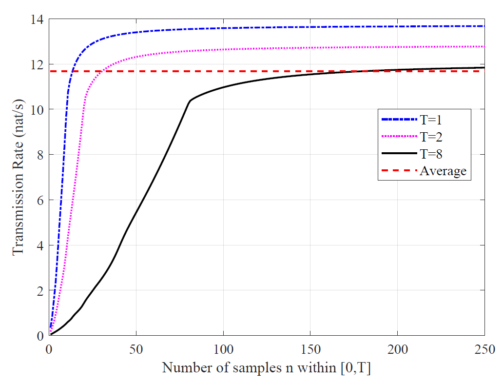
We calculate the finite-time transmission rate $C(T)$ and the average mutual information $C_{\rm av}$ against the number of samples $n$ within the observation window $[0,T]$. The numerical results are collected in Fig. 1. It is shown that $I(t_{1}^{n})$ is an increasing function of $n$, and for fixed values of $T$, the approximated finite-time mutual information $I(t_{1}^{n})$ tends to a finite limit under the correlation assumptions given by (5). The most amazing observation is that, it is possible to obtain more information within finite-time window $[0,T]$ than the prediction $TC_{\rm av}$ given by averaging the mutual information along the entire time axis (6). We call this phenomenon the exceed-average phenomenon.

By analyzing the structure of the autocorrelation functions, it is possible to obtain $I(t_{1}^{n})$ and $I(T)$ directly. In fact, if we know the Mercer expansion [6] of the autocorrelation function $R_{X}(t_{1},t_{2})$ on interval $[0,T]$, then we can calculate $h({\bm{X}}(t_{1}^{n}))$ more easily [9]. In the following discussion, we assume the Mercer expansion of the source autocorrelation function $R_{X}(t_{1},t_{2})$ to be in the following form

where the eigenvalues are positive: $\lambda_{k}>0$, and the eigenfunctions form an orthonormal set:

The Mercer’s theorem [6] ensures the existence and uniqueness of the eigenpairs $(\lambda_{k},\phi_{k}(t))_{k=1}^{\infty}$, and furthermore, the kernel itself can be expanded under the eigenfunctions:

Based on Mercer expansion, we obtain a closed-form formula in the following Theorem 1.

From Theorem 1 we can conclude that the finite-time mutual information of AWGN channel is uniquely determined by the Mercer spectra $\lambda_{k}$ of $R_{X}(t_{1},t_{2})$ within $[0,T]$. However, it remains unknown whether the series representation (10) converges. In fact, the convergence is closely related to the signal power, which is calculated in the following Lemma 1.

To prove the exceed-average phenomenon, we only need to show that the finite-time mutual information is greater than the averaged mutual information in a typical case. Let us consider a finite-time communication scheme with a finitely-powered stationary transmitted signal autocorrelation²²2The signal autocorrelation $R_{X}(\tau)$ is often observed in many scenarios, such as passing a signal with white spectrum through an RC lowpass filter., which is specified as

where $\tau=t_{1}-t_{2}$, under AWGN channel with noise PSD being $n_{0}/2$. The power of signal $X(t)$ is $P=R_{X}(0)$. According to Lemma 1, the trace of the corresponding Mercer operator $M(\cdot)$ is finite. Then the finite-time mutual information given by Theorem 1 is also finite, as is shown in Remark 1. Finding the Mercer expansion is equivalent to finding the eigenpairs $(\lambda_{k},\phi_{k}(t))_{k=1}^{\infty}$. The eigenpairs are determined by the following characteristic integral equation [10]:

Differentiating both sides of (13) twice with respect to $s$ yields the boundary conditions and the differential equation that $\lambda_{k},\phi_{k}$ must satisfy:

Let $\omega_{k}>0$ denote the resonant frequency of the above harmonic oscillator equation, and let $\phi_{k}(t)=A_{k}\cos(\omega_{k}t)+B_{k}\sin(\omega_{k}t)$ be the sinusoidal form of the eigenfunction. Using the boundary conditions we obtain

To ensure the existence of solution to the homogeneous linear equations (15) with unknowns $A_{k},B_{k}$, the determinant must be zero. Exploiting this condition, we find that $\omega_{k}$ naturally satisfy the transcendental equation $\tan(\omega_{k}T)=(2\omega_{k}\alpha)/({\omega_{k}^{2}-\alpha^{2}})$. By introducing an auxillary variable $\theta_{k}=\arctan(\omega_{k}/\alpha)\in[0,\pi/2]$, this transcendental equation can be simplified as $\tan(\omega_{k}T)=-\tan(2\theta_{k})$, i.e., there exists positive integer $m$ such that $2\arctan(\omega_{k}/\alpha)=m\pi-\omega_{k}T$. The integer $m$ can be chosen to be equal to $k$. From the function images of $2\arctan(\omega/\alpha)$ and $k\pi-\omega T$ (Fig. 2), we can determine $\omega_{k}$, and then $\lambda_{k}$. To sum up, the solution to the characteristic equation (13) are collected into (16) as follows.

where $Z_{k}$ denotes the normalization constants of $\phi_{k}(t)$ on $[0,T]$ to ensure orthonormality.

Equation (16) gives all the eigenpairs $(\lambda_{k},\phi_{k})_{k=1}^{\infty}$, from which we can calculate $I(T)$ by applying Theorem 1. As for the Shannon limit $C_{\rm sh}$, by applying (6) and evaluating the integral with [11] we can obtain

After all the preparation works above, we can rigorously prove that $C(T)>C_{\rm av}$ under the typical case of (12), as long as the transmission power $P$ is smaller than a constant $\delta$. The following Theorem 2 proves this result.

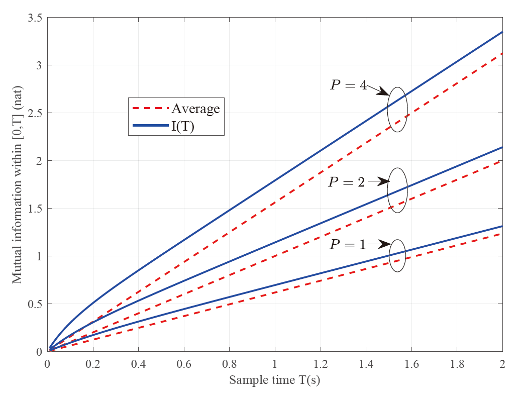
To support the above theoretical analysis, numerical experiments on $I(T)$ are conducted based on evaluations of (16) and (17). As shown in Fig. 3, it seems that we can always harness more mutual information in a finite-time observation window than the averaged mutual information. This fact is somehow unsurprising because the observations ${\bm{Y}}(t_{1}^{N})$ inside the window $[0,T]$ can always eliminate some extra uncertainty outside the window due to the autocorrelation of $X(t)$.

Though the exceed-average effect do imply mathematically that the mutual information within a finite-time window is higher than the average mutual information $C_{\rm av}$ (which coincides with the Shannon limit (6) in this case), in fact, it is still impossible to construct a long-time stable data transmission scheme above the Shannon capacity by leveraging this effect. So the exceed-average phenomenon does not contradict the Shannon-Hartley Theorem. Placing additional observation windows cannot increase the average information rate, because the posterior process $Y(t)|{\bm{Y}}(t_{1}^{N})$ does not carry as much information as the original one, causing a rate reduction in the later windows. It is expected that, the finite-time mutual information would ultimately decrease to the average mutual information as the total observation time tends to infinity (i.e., $C(\infty)=C_{\rm av}$), and the analytical proof, as well as the achievability of this finite-time mutual information, is still worth investigation in future works.

References

- [1] C. E. Shannon, “A mathematical theory of communication,” The Bell Syst. Techni. J., vol. 27, no. 3, pp. 379–423, Jul. 1948.
- [2] H. Landau, “Sampling, data transmission, and the nyquist rate,” Proc. IEEE, vol. 55, no. 10, pp. 1701–1706, Oct. 1967.
- [3] H. Nyquist, “Certain topics in telegraph transmission theory,” Trans. American Institute of Electrical Engineers, vol. 47, no. 2, pp. 617–644, Apr. 1928.
- [4] D. Slepian, “On bandwidth,” Proc. IEEE, vol. 64, no. 3, pp. 292–300, Mar. 1976.
- [5] T. M. Cover, Elements of information theory. John Wiley & Sons, 1999.
- [6] J. Mercer, “Functions of positive and negative type and their connection with the theory of integral equations,” Philos. Trans. Royal Soc., vol. 209, pp. 4–415, 1909.
- [7] K. Zhu, Operator theory in function spaces. American Mathematical Soc., 2007, no. 138.
- [8] A. Balakrishnan, “A note on the sampling principle for continuous signals,” IRE Trans. Inf. Theory, vol. 3, no. 2, pp. 143–146, Jun. 1957.
- [9] J. Barrett and D. Lampard, “An expansion for some second-order probability distributions and its application to noise problems,” IRE Trans. Inf. Theory, vol. 1, no. 1, pp. 10–15, Mar. 1955.
- [10] D. Cai and P. S. Vassilevski, “Eigenvalue problems for exponential-type kernels,” Comput. Methods in Applied Math., vol. 20, no. 1, pp. 61–78, Jan. 2020.
- [11] I. S. Gradshteyn and I. M. Ryzhik, Table of integrals, series, and products. Academic press, 2014.