On explicit geometric solutions of some inviscid flows with free boundary.
Abstract
The aim of this paper is to discuss some well known explicit examples of the three dimensional inviscid flows with free boundary constructed by John [John] and Ovsyannikov [Ovsyannikov], and provide a detailed analysis of its long time behaviour.
1 Introduction
The aim of this paper is to discuss some well known explicit examples of the three dimensional inviscid flows with free boundary constructed by John [John] and Ovsyannikov [Ovsyannikov], and provide a detailed analysis of its long time behaviour. It is rare to have such explicit examples of flows even in the two dimensional case [Higgins], [Gilbarg], which among other things, makes these solutions special as they describe the instability of the free boundary as . It is important to note that in all these examples the free boundary, regarded as a surface, is a conic section.
In section 2 we study an irrotational inviscid flow from [Ovsyannikov] where the free boundary is a round cylinder. This example provides an explicit asymptotics in time exhibiting blow up in finite time and shrinking to a line in infinite time.
In section 3 and 4 we provide a similar analysis for the solutions of John [John]. The time asymptotics results are new and did not appear in [John].
Finally, in section 5 we discuss the case of rotational flow [Ovsyannikov], which in finite time transform from unit sphere to an ellipsoid and then back to sphere, after which the flow continues as a needle that collapses to a plane at infinity.
For each , let be the moving domain containing the fluid. Denote the Cartesian coordinates as , and let be the velocity vector field. Suppose the flow is incompressible, i.e. . Moreover, we also assume the flow is irrotational, i.e. . Then there exists such that . This then implies that
| (1.1) |
Moreover, the flow at free boundary is modelled by the two postulations:
-
(i)
The free boundary is following the particle path (Kinematic equation);
-
(ii)
The Bernoulli’s principle is satisfied at the free boundary (Dynamic equation).
Formulation of kinematic equation.
Let be a point on that moves along with the free boundary. Then postulation (i) indicates that
| (1.2) |
Suppose that the moving domain is described by the implicit inequality of the form:
for some function . Then the free boundary is determined by
Since is a point on the surface, it follows that for all . Thus by chain rule, we obtain:
| (1.3) |
In particular, for each given point , let be the backward characteristic satisfying
| (1.4) |
Then the following differential equation also holds:
| (1.5) |
Formulation of dynamic equation.
The Bernoulli’s principle at the surface is:
where is the pressure. In the present paper, we consider the model for which there is no surface tension. Then for some function of time .
In summary the incompressible irrotational flow with free boundary is governed by the following system of equations
| (1.6a) | ||||
| (1.6b) | ||||
| (1.6c) | ||||
Since the domain is entirely determined by , (1.6) is a system of equations with unknowns, which are , , and .
Acknowledgements
The authors were partially supported by EPSRC grant EP/S03157X/1 Mean curvature measure of free boundary.
2 Flow of Cylinder
In this section, we present the explicit solution to (1.6) first obtained by Ovsjannikov in [Ovsyannikov]. For a function , and constant , we consider the following ansatz for potential function:
| (2.1) |
It can be easily verified that . Here we are looking for a free boundary taking the form of cylinder, which means that the surface is described by the equation of the form:
| (2.2) |
Inferences from the surface evolution equation (1.6b).
Suppose that the equation describes the free boundary surface. For a given time , fix . Let be the backward characteristic curve emanating from , i.e. solves (1.4). Using the ansatz (2.1), one has
Solving the above ODEs we have for ,
Suppose that at , the initial configuration for the free boundary is determined by a given function , i.e. , Then it follows that
| (2.3) |
Thus the general equations for the free surface takes the form (2.3), with being a function independent of the variables .
Inferences from the Bernoulli’s principle (1.6c).
Substituting the ansatz (2.1) into the Bernoulli’s principle (1.6c), one has
| (2.4) |
Since we are seeking free boundaries taking the form of a cylinder described in (2.2), we impose that the coefficient for in (2.4) must be zero, which implies
Hence , which then gives where we denote . Solving this ODE, it has the solution:
| (2.5) |
Substituting this into (2.4), one has
| (2.6) |
In addition, putting (2.5) into (2.3), it implies that the free surface must take the form:
| (2.7) |
Since (2.6) and (2.7) must be consistent, it follows that there exists some constant such that . Suppose , then . Thus,
Therefore the free surface is described by the equation , with
Time Asymptotic.
The behaviour of free surface can be categorised into two cases: and . If then the radius of free surface blows up to infinity in finite time as . If , then the radius is shrinking to as .
3 Flow of Ellipsoid, Hyperboloid, and Cone
We solve (1.6) assuming that potential function takes the following form:
| (3.1) |
This ansatz was first proposed and studied by F. John in [John].
3.1 ODE for
Inferences from the surface evolution equation (1.6b).
Suppose that the equation describes the moving free boundary surface. For at time , let be the backward characteristic curve emanating from . Then for all . Putting the ansatz (3.1) into the differential equation (1.4), one has
For simplicity, denote for . Then solving this, one has
Suppose that at , the initial configuration for the free boundary is determined by a given function , i.e. , Then it follows that
| (3.2) |
Thus the general equations for the free surface takes the form (3.2), with being function independent of the variables .
Inferences from the Bernoulli’s principle (1.6c).
Substituting the ansatz (3.1) into the Bernoulli’s principle (1.6c), one has
Rewriting the above equally in accordance to (3.2), we have
| (3.3) |
Two equations (3.2) and (3.3) must be consistent, which means that we must have
| (3.4) |
for some fixed constants . The first equation of the above can be rewritten as . Taking derivative, and noting that , one gets
| (3.5) |
Multiplying the above with we have that . Applying the partial fraction decomposition on the left hand side of this equation, we have
Multiplying the above with , then integrating the resultant equation we obtain that
| (3.6) |
with . Next, substituting into the second equation of (3.4), then using (3.6), we also obtain that for ,
| (3.7) |
3.2 Solution for and convergence behaviour
Expanding the identity (3.6), one obtains . Setting . Then we obtain the depressed cubic equation of the form:
| (3.8) |
We consider the quantity
By the formula for depressed cubic equations, if then (3.8) has 1 real root and 2 complex roots, and the real root in this case can be obtained using Cardano’s formula
| (3.9) |
Furthermore, this real root can also be represented in terms of hyperbolic function:
| (3.10) |
where denotes the sign function. On the other hand, if then it has 3 distinct real roots, and if then it has 2 distinct real roots with one of them having multiplicity 2. In these cases, the solution is given by Viète’s trigonometric formula
| (3.11) |
Setting . By the definition of in (3.6), it follows that
| (3.12) |
Suppose that is continuous near . Then for small time , one has . Therefore according to (3.12), the root of (3.8) on a neighbourhood of is given by Cardano’s formula (3.9) if , and Viète’s formula (3.11) if . It can be verified that for and for . Therefore we split the analysis into 2 cases:
Case 1: .
The root for (3.8) is given by one of the three possible solutions of Viète’s trigonometric formula (3.11):
| (3.13) |
for . The relevant integer must be chosen so that solution satisfies the initial condition . By the definition of in (3.12), it can be verified that for . Using this, we have
Therefore, depending on the initial data , solves the differential equation:
| (3.14) |
Integrating the above in , and by the fact that , we have for ,
| (3.15) |
Let be the maximal time for which is invertible. Then
| (3.16) |
Case 2: .
In this case, the one physical real root for (3.8) is given by the Cardano’s formula (3.9):
| (3.17a) | ||||
| where | (3.17b) | |||
| We remark that can also be represented in terms of hyperbolic function | ||||
| (3.17c) | ||||
Let , then satisfies the differential equation
| (3.18) |
Integrating the above in , and using we have that for ,
| (3.19) |
Using the integral expressions (3.15) and (3.19), one can numerically plot the curve , which is then analysed to determine the convergence of as . Without loss of generality, we restrict our analysis to the case . The case can be obtained by the transformation: , which preserves the differential equations (3.5)–(3.6). We consider initial data in distinct regimes. The statements and figures listed below, describing the behaviour of as are based on the numerical integration of (3.15) and (3.19).
Regime 1: .
In this case, and the differential equation is given by . Moreover, (3.6) implies that and is monotone decreasing due to and (3.5). From the fact that and (3.6), it follows that as increases from , one has the limit and . On the other hand, as decreases from , one has the limit and where . Thus, we aim to find the times: for which , and for which . By the numerical simulation, we have
-
fnum@enumiitem (i)(i)
For the case of increasing , the integral (3.19) converges to a positive finite time: as . Thus in finite time as .
-
fnum@enumiitem (ii)(ii)
For the case of decreasing , the integral (3.19) converges to a negative finite time: as . Thus in finite time as . In this scenario, we take as an initial data starting in Regime 2(ii) then concatenate the resulting solution with .

Figure 3.1: the plot of curve with for Regime 1. Regime 2: .
In this case, and solves according to (3.14). Moreover, (3.6) implies that , and is monotone decreasing since and (3.5). From the fact that and (3.6), it follows that as increases from , one has the limit and , where . On the other hand, as decreases from , one has the limit and . Thus, we aim to find the times for which , and for which . According to the numerical simulation, we have
-
fnum@enumiiitem (i)(i)
For the case of increasing , the integral (3.15) converges to a positive finite time: as . Thus in finite time as . In this scenario, we take as an initial data starting in Regime 1(i) then concatenate the resulting solution with .
-
fnum@enumiiitem (ii)(ii)
For the case of decreasing , it can be verified that as . Hence the integral (3.15) diverges to negative infinity: as , which implies that . Thus in infinite time as .

Figure 3.2: the plot of curve with for Regime 2. 
Figure 3.3: the plot of curve with for Regime 3. Regime 3: .
In this case, and the differential equation is given by according to (3.14). Moreover, (3.6) implies that , and is monotone increasing since and (3.5). From the fact that and (3.6), it follows that as increases from , one has the limit and , where . On the other hand, as decreases from , one has the limit and . Thus, we aim to find the times for which , and for which . According to the numerical simulation, we have
-
fnum@enumiiiitem (i)(i)
For the case of increasing , the integral (3.15) converges to a positive finite time: as . Thus in finite time as . In this scenario, we take as an initial data starting in Regime 4(i) then concatenate the resulting solution with .
-
fnum@enumiiiitem (ii)(ii)
For the case of decreasing , it can be verified that as . Hence the integral (3.15) diverges to negative infinity: as , which implies that . Thus as .
Regime 4: .
In this case, and the differential equation is given by according to (3.14). Moreover, (3.6) implies that , and is monotone increasing since and (3.5). From the fact that and (3.6), it follows that as increases from , one has the limit and . On the other hand, as decreases from , one has the limit and , where . Thus, we aim to find the times for which , and for which . By the numerical simulation, we have
-
fnum@enumivitem (i)(i)
For the case of increasing , it can be verified that as . Hence the integral (3.15) diverges to positive infinity: as , which implies that . Thus in infinite time as .
-
fnum@enumivitem (ii)(ii)
For the case of decreasing , the integral (3.15) converges to a negative finite time: as . Thus in finite time as . In this scenario, we take as an initial data starting in Regime 3(ii) then concatenate the resulting solution with .
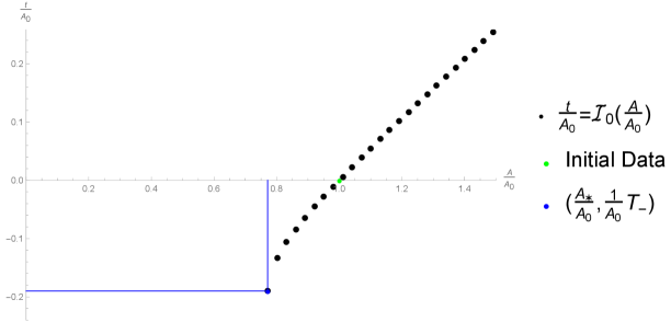
Figure 3.4: the plot of curve with for Regime 4. Regime 5: .
In this case, and the differential equation is given by . Moreover, (3.6) implies that , and is monotone decreasing since and (3.5). From the fact that and (3.6), it follows that as increases from , one has the limit and . On the other hand, as decreases from , one has the limit and . Thus, we aim to find the time for which . From (3.6), we see that as , and for which . By the numerical simulation, we have
-
fnum@enumv(i)(i)
For the case of increasing , it can be verified that as . Hence the integral (3.19) diverges to positive infinity: as , which implies that . Thus in infinite time as .
-
fnum@enumv(ii)(ii)
For the case of decreasing , the integral (3.19) converges to a negative finite time: as . Thus in finite time as .

Figure 3.5: the plot of curve with for Regime 5. 3.3 Free boundary surface and phase space
The free boundary surface of the flow is determined by (3.3), (3.6), and (3.7). This is stated as:
(3.20) with and . From this, we see that
-
•
If or , then the surface is either an one-sheeted or two-sheeted hyperboloid, or a cone;
-
•
If , then the surface is an ellipsoid.
For a given initial data and , the solution to (3.5)–(3.6) exists up to the maximum time of existence and or due to the construction given in the previous section. In what follows, we study the evolution of its corresponding free surface. Once again, due to the time symmetry of the differential equations (3.5)–(3.6) for , we restrict our analysis to the case . We split the initial data into 9 cases:
Case I(a): and . The initial free boundary is an One-Sheeted Hyperboloid.
In this case, and . Rewriting (3.20) using (3.6), we have
(3.21) By the analysis of Regime 1 and Regime 2 in the previous section, we have
-
fnum@enumvi(i)(i)
For increasing , there exists a finite time such that , as . Thus, as , the free surface converges to an One-Sheeted Hyperboloid given by the following equation:
-
fnum@enumvi(ii)(ii)
For decreasing , we have the limit , as . Thus, as , the free surface collapses to the -axis described by the equation .
Case I(b): and . The initial free boundary is a Two-Sheeted Hyperboloid.
In this case, and . The evolution of surface is described by the same equation as (3.21). According to Regime 1 and Regime 2, we have
-
fnum@enumvii()()
For increasing , there exists a finite time such that , as . Thus, as , the free surface converges to a Two-Sheeted Hyperboloid given by the following equation
-
fnum@enumvii()()
For decreasing , we have the limit , as . Thus, as , the free surface collapses to the -axis described by the equation .
Case I(c): and . The initial free boundary is a Cone.
In this case, and . The evolution of surface is described by the same equation as (3.21). By the analysis of Regime 1 and Regime 2 in the previous section, we have
-
fnum@enumviii()()
For increasing , there exists a finite time such that , as . Thus, as , the free surface converges to a Cone with slope given by the equation
-
fnum@enumviii()()
For decreasing , we have the limit , as . Thus, as , the free surface collapses to the -axis described by the equation .
Case II: and . The initial free boundary is an Ellipsoid or a point.
The free surface is described by (3.20) and solution as
If then (3.20) reduces to the equation which describes a point at the origin. In addition, we remark that is not possible in this case. By the analysis of Regime 3 and Regime 4 in the previous section, we have
-
fnum@enumix()()
For increasing , we have , as . Therefore in the limit , the equation (3.20) reduces to , which means that the free surface collapses into the -Plane.
-
fnum@enumix()()
For decreasing , we have the limit , as . Thus, as , the free surface collapses to the -Axis described by the equation .
Case III(a): and . The initial free boundary is a Two-Sheeted Hyperboloid.
In this case, and . The free surface is described by the same equation as (3.21). By the analysis of Regime 5 in the previous section, we have
-
fnum@enumx()()
For increasing , we have , as . Taking this limit in (3.20), the equation reduces to as . Thus, the free surface collapses to the (x,y)-Plane in the limit .
-
fnum@enumx()()
For decreasing , there exists a finite time such that , as . Thus, as , the free surface converges to a Two-Sheeted Hyperboloid described by the equation:
Case III(b): and . The initial free boundary is an One-Sheeted Hyperboloid.
In this case, and . The free surface is described by the same equation as (3.21). According to Regime 5 in the previous section, we have
-
fnum@enumxi()()
For increasing , we have , as . Taking this limit in (3.20), the equation reduces to as . Thus, the free surface collapses to the (x,y)-Plane in the limit .
-
fnum@enumxi()()
For decreasing , there exists a finite time such that , as . Thus, as , the free surface converges to an One-Sheeted Hyperboloid described by the equation:
Case III(c): and . The initial free boundary is a Cone.
In this case, and . The free surface is an evolving cone described by the same equation as (3.21). By the analysis in Regime 5, we have
-
fnum@enumxii()()
For increasing , we have , as . Taking this limit in (3.20), the equation reduces to as . Thus, the free surface collapses to the (x,y)-Plane in the limit .
-
fnum@enumxii()()
For decreasing , there exists a finite time such that , as . Thus, as , the free surface converges to the Cone with slope described by the equation:
Case IV: and . The initial free boundary is the -axis.
For this initial data, and the solution is explicitly given by . The equation (3.20) for the surface remains as the -Axis given by the equation .
Case V: and . The initial free boundary is a Two-Sheeted Plane perpendicular to the -axis.
For this initial data, and . The solution is explicitly given by , and the equation (3.20) for the surface is:
This describes a two-sheeted plane perpendicular to the -axis moving along the -direction with velocities . Note that in this case is impossible.
![[Uncaptioned image]](https://cdn.awesomepapers.org/papers/524b9f58-8437-43a6-bdc1-eb33a996abd6/x6.png)
Remark 3.1.
The point for which and cannot exist as a solution to (3.6). Thus the set is excluded from the phase space of .
3.4 Time asymptotic of
In this section, we study the time asymptotic behaviour of and . As before, we restrict our study to the case since the solution for can be obtained by the transformation: .
Time asymptotic for Case I.
The initial data in this case satisfies and . According to Regime 1(i) and Regime 2(i), if we set
then as . It follows from (3.19) that
(3.22) Since , (3.12) implies that . By the expression (3.17), the following series expansion holds:
Substituting the above into (3.22), it follows that as ,
Therefore we obtain the convergence rate
Combining the above convergence rate with (3.17), we conclude that
Next, we consider the asymptotic of in the limit . According to the analysis given in Regime 1(ii) and Regime 2(ii), as , takes the form:
(3.23) It can be verified that . This implies . Hence its inverse satisfies . In addition, there exists such that for all , , hence
Thus we have . For inverse function , we have that
Therefore we conclude
Since , by inverse function theorem,
The following series expansion holds:
Using these in the expression (3.23), we obtain the series expansion:
Applying the fact that as , we conclude that
In summary if and , then the corresponding solution satisfies the following asymptotic behaviour: there exists such that
Time asymptotic for Case II.
The initial data in this case satisfies and . According to the analysis given in Regime 3(i) and Regime 4(i), in the limit , the solution is takes the form:
(3.24) It can be verified that . This implies . Hence its inverse satisfies . In addition, there exists such that for all , , hence
Thus we have . For inverse function , we have that
Therefore we conclude
Since , by inverse function theorem,
The following series expansion holds:
Using these in the expression (3.24), we obtain the series expansion:
Applying the fact that as , we conclude that
Next we consider the asymptotic behaviour of , in the limit . In this case, according to Regime 3(ii) and Regime 4(ii), the solution is given by
(3.25) It can be verified that . This implies . Hence its inverse satisfies . In addition, there exists such that for all , , hence
Thus we have . For inverse function , we have that
Therefore we conclude
Since , by inverse function theorem,
The following series expansion holds:
Using these in the expression (3.25), we obtain the series expansion:
Applying the fact that as , we conclude that
In summary, if and , then the corresponding solution satisfies the following time asymptotic behaviour:
Time asymptotic for Case III.
The initial data in this case satisfies and . According to Regime 5(i), as , the solution takes the form:
where is defined in (3.17). It can be verified that . This implies . Hence its inverse satisfies . In addition, there exists such that for all , , hence
Thus we have . For inverse function , we have that
Therefore we conclude
Since , by inverse function theorem,
From (3.17), one has the following series expansion:
Applying the fact that as , we conclude that
Next, we consider the asymptotic of as decreases. According to the analysis given in Regime 5(ii), if we set
then as . It follows from (3.19) that
(3.26) Since , (3.12) implies that . By the expression (3.17), the following series expansion holds:
Substituting the above into (3.26), it follows that as ,
Therefore we obtain the convergence rate
Combining the above convergence rate with (3.17), we conclude that
In summary if and , then the corresponding solution satisfies the following asymptotic behaviour: there exists such that
4 Flow of Parabola with Drift
Suppose that is a solution to (3.5)–(3.6). We consider the following ansatz:
(4.1) For each point at time , let be the backward characteristic curve emanating from , which satisfies and the differential equations
For simplicity denote for . Solving these, one has
(4.2) Therefore, the equation describing the free surface must satisfies the form:
(4.3) for some function independent of . On the other hand, substituting (4.1) into (1.6c), we have
(4.4) Rewriting the above in terms of given in (4.2), one obtains
Since the above equation must be consistent with (4.3), it follows that there exists constants , , such that
(4.5a) (4.5b) (4.5c) From (4.5a), we have the identity . Substituting this into (4.5b),
Taking derivative on the above equation, and using the definition , we obtain
Using the identity on the above equation once again, then rearranging terms, we have
(4.6) Assuming further that where , then one has the equation
In addition, using the expression (4.5c), one can calculate to get that c(t)-B22 = ( c_0 - B022 )a03(a0-t)3. where . Substituting these expression of and into (4.4), we conclude that the free surface is a Paraboloid described by the equation
(4.7) As , this paraboloid will collapse to -Axis described by .
5 Flow of Ellipsoid with Constant Vorticity
In this section we construct an explicit solution to (1.6b)–(1.6c) with vorticity, i.e. when the condition (1.6a) is not satisfied. More precisely, the solution has constant vorticity for some constant . We remark that such solution was first studied by Ovsjannikov in [Ovsyannikov].
Let be the position vector of the free surface at time , and denote . We impose the following ansatz:
(5.1) Here are functions of such that with being the -by- identity matrix. Let be the pressure. By chain rule one has,
Then Newton’s second law yields
Substituting the ansatz into the above equation, we obtain that,
Integrating in and noting that on the free surface, pressure is constant for given time , we get that
In addition, we also impose the following similarity relations:
(5.2) Our aim is then to find and that solve the problem with initial conditions:
(5.3) Since is also the particle trajectory, if we set as the velocity, then
From the incompressibility , and Jacobi’s formula for determinant, one has
It follows that , hence by (5.1),
(5.4) Next, by a direct computation one has
Then the similarity assumption (5.2) yields
(5.5) From here, we wish to reduce the system into a single ODE for and solve it. Using (5.5), we get that hence after integration we have
Moreover, differentiating (5.4), we have . Putting these equations together, it forms the system:
(5.6) (5.7) Multiplying the first equation by , and the second one by and adding up we get , or equivalently
Utilizing (5.4) we obtain
Repeating the same calculation but with and exchanged, we also obtain
Using the last two equations and (5.4) one more time we get that
(5.8) Differentiating (5.7) yields
Substituting (5.5) and (5.8) into the above, we obtain
Hence we get the desired ODE for
(5.9) In order to solve (5.9) we make the substitution , for a new unknown . Then solves the following first order ODE
Note that
This yields,
Recalling the definition of , we finally get
Denote , then
(5.10) We immediately see that . Using the initial condition , we get that
For this case, if and close to , must be increasing. Thus integrating (5.10), we have
As increases, it attains the value at , where is determined from
From (5.9) and (5.10) it follows that has a local maximum at , and decrease for . For these values of we have
From here it follows that as then . The graph of is shown in Figure 5.6.

Figure 5.6: The plot of . The functions can be calculated as functions of as follows: in light of the incompressibility condition (5.4), and constant vorticity condition (5.6), we let
To determine , we use (5.6) to obtain that
Now let us discuss the geometric picture for this flow. The pressure can be assumed zero on the sphere , and the mapping given by the matrix implies
We see that for the sphere at turns into an ellipsoid of revolution with axis until the moment when its major semiaxis becomes equal to . After that the ellipsoid reverses its motion back to the unit sphere, and consequently flattens out to the plane , as (see Figure 5.6). The 3D animation of this flow can be viewed here; https://www.maths.ed.ac.uk/~aram/mov.html .
To clarify the mechanical phenomenon, let us look at the velocity at initial data. Since , and , we have
Observe that the matrix is not symmetric, which indicates that the motion is not irrotational. In fact . Therefore the initial state of the motion, at , corresponds to uniform rotation of the sphere about axis with angular velocity If then we get a potential flow discussed earlier, for which the needle stretches to a line as . However, for , the stretching into line is impossible and the flow collapses to a hyperplane, as explained above.
The velocity at every point can be written in the form , where is a potential function and is the rotation component about the -axis. The kinematic energy of the system is the sum of kinetic energies
During the flow transfers to up to the point , where , after that the transfer reverses its direction from to as , until it purges and gives and .
References
-
fnum@enumxii()()
-
fnum@enumxi()()
-
fnum@enumx()()
-
fnum@enumix()()
-
fnum@enumviii()()
-
fnum@enumvii()()
-
•
-
fnum@enumv(i)(i)
-
fnum@enumivitem (i)(i)
-
fnum@enumiiiitem (i)(i)
-
fnum@enumiiitem (i)(i)