On Controllability and Persistency of Excitation in Data-Driven Control: Extensions of Willems’ Fundamental Lemma
Abstract
Willems’ fundamental lemma asserts that all trajectories of a linear time-invariant system can be obtained from a finite number of measured ones, assuming that controllability and a persistency of excitation condition hold. We show that these two conditions can be relaxed. First, we prove that the controllability condition can be replaced by a condition on the controllable subspace, unobservable subspace, and a certain subspace associated with the measured trajectories. Second, we prove that the persistency of excitation requirement can be relaxed if the degree of a certain minimal polynomial is tightly bounded. Our results show that data-driven predictive control using online data is equivalent to model predictive control, even for uncontrollable systems. Moreover, our results significantly reduce the amount of data needed in identifying homogeneous multi-agent systems.
I Introduction
Willems’ fundamental lemma provides a data-based parameterization of trajectories generated by linear time invariant (LTI) systems [1]. In particular, consider the LTI system
| (1a) | ||||
| (1b) | ||||
where denote the input, state and output of the system at discrete time , respectively. If system (1) is controllable, the lemma asserts that every length- input-output trajectory of system (1) is a linear combination of a finite number of measured ones. These measured trajectories can be extracted from one single trajectory with persistent excitation of order [1], or multiple trajectories with collective persistent excitation of order [2]. By parameterizing trajectories of the system (1) using measured data, the lemma has profound implications in system identification [3, 4, 5], and inspired a series of recent results including data-driven simulation [3, 6], output matching [7], control by interconnection [8], set-invariance control [9], linear quadratic regulation [10], and predictive control [11, 12, 13, 14, 15, 16, 17].
In the meantime, whether conditions of controllability and persistency of excitation in Willems’ fundamental lemma are necessary has not been investigated in depth. The current work aims to address this issue by answering the following two questions. First, without controllability, to what extent can the linear combinations of a finite number of measured input-output trajectories parameterize all possible ones? Second, can the order of persistency of excitation be reduced?
Recent results on system identification has shown that, assuming sufficient persistency of excitation, the linear combinations of a finite number of measured input-output trajectories contain any trajectory whose initial state is in the controllable subspace [18, 19]. As we show subsequently, such results only partially answer the first question above: trajectories with initial state outside the controllable subspace can also be contained in said linear combinations.
We answer the aforementioned questions by introducing extensions of Willems’ fundamental lemma. First, we show that, with sufficient persistency of excitation, any length- input-output trajectory whose initial state is in some subspace is a linear combination of a finite number of measured ones. Said subspace is the sum of the controllable subspace, unobservable subspace, and a certain subspace associated with the measured trajectories. Second, we show that the order of persistency of excitation required by Willems’ fundamental lemma can be reduced from to , where is the degree of the minimal polynomial of the system matrix . Our first result completes those presented in [18, 19] by showing exactly which trajectories are parameterizable by a finite number of measured ones for an arbitrary LTI systems. Furthermore, this result shows that data-driven predictive control using online data is equivalent to model predictive control, not only for controllable systems, as shown in [12, 13], but also for uncontrollable ones. Our second result, compared with those in [2], can reduce the amount of data samples used in identifying homogeneous multi-agent systems by an order of magnitude.
The rest of the paper is organized as follows. We first prove an extended Willems’ fundamental lemma and discuss its implications in Section II. We provide ramifications of this extension for a representative set of applications in Section III before providing concluding remarks in Section IV.
Notation: We let , and and denote the set of real numbers, non-negative integers, and positive integers, respectively. The image and right kernel of matrix is denoted by and , respectively. Let for any matrix and vector . When applied to subspaces, we let and denote the sum [20, p.2] and Cartesian product operation [20, p.370], respectively. We let denote the Kronecker product. Given a signal and with , we denote , and the Hankel matrix of depth () associated with as
II Extensions of Willems’ fundamental lemma
In this section, we introduce extensions of Willems’ fundamental lemma. Throughout we let
| (2) |
denote a length- () input-state-output trajectory generated by system (1) for all , where is the total number of trajectories. We let
| (3) |
denote the set of input, state, and output trajectories, respectively. We will use the following subspaces,
| (4) | ||||
where , and is the first state in the trajectory for all . In particular, is known as the controllable subspace (we say that system (1) is controllable if ), is known as the unobservable subspace, and is the smallest -invariant subspace containing . Using the Cayley-Hamilton theorem, one can verify that (1) ensures
| (5) |
for all , where is defined similar to . We let be such that
| (6) |
where is the minimal polynomial of matrix [20, Def. 3.3.2], and, due to the Cayley-Hamilton theorem, is upper bounded by . We will also use the following definitions that streamline our subsequent analysis.
Definition 1.
We say a length- input-output trajectory , with , is parameterizable by if there exists such that
| (7) |
As an example, if , , , then (7) assumes the form,
Definition 2 (Collective persistent excitation [2]).
We say that is collectively persistently exciting of order if for all , and the mosaic-Hankel matrix,
| (8) |
has full row rank.
The Willems’ fundamental lemma asserts that: if the system (1) is controllable and is collectively persistently exciting of order , then is parameterizable by if and only if it is an input-output trajectory of the system (1) [1, 2]. As our main contribution, the following theorem shows that not only the controllability assumption can be relaxed, but also the required order of collective persistent excitation can be reduced from to, at best, .
Theorem 1.
Let be a set of input-state-output trajectories generated by the system (1). If is collectively persistently exciting of order where satisfies (6), then
| (9) | ||||
Further, is parameterizable by if and only if there exists a state trajectory with
| (10) |
such that is an input-state-output trajectory generated by (1).
Proof.
See the Appendix. ∎
Remark 1.
Due to its dependence on state and the unknown subspaces in (4), the condition in (10) is difficult to verify, especially if merely input-output trajectories are available. One approach to guarantee its satisfaction is to ensure the right hand side of (10) equals , either by assuming controllability (i.e., ) as in [1] and [2], or requiring the input-state-output trajectories in (2) satisfy . The following corollary, however, provides an alternative approach that requires neither controllability nor state measurements.
Corollary 1.
Proof.
See the Appendix. ∎
Corollary 1 shows that any length- segment of an input-output trajectory is parameterizable by its first length- segment, assuming sufficient persistency of excitation. This result is particularly useful in predictive control as we will show in Section III-A.
Another implication of Theorem 1 is that the order of persistent excitation required by trajectory parameterization only depends on the degree of the minimal polynomial of matrix in (1), instead of its dimension. In general, it is difficult to establish a bound on the degree of the minimal polynomial of an unknown matrix tighter than its dimension. However, the following corollary shows an exception; its usefulness will be illustrated later in Section III-B.
Corollary 2.
If there exists such that , where , then Theorem 1 holds with .
The proof follows from Theorem 1 and the fact that the minimal polynomial of is the same as that of , which has degree at most .
III Applications
In this section, we provide two examples that illustrate the distinct implications of Theorem 1.
III-A Online data-enabled predictive control
Model predictive control (MPC) provides an effective control strategy for systems with physical and operational constraints [21, 22]. In particular, consider system (1) with output feedback. At each sampling time , given the input-output measurements history , MPC solves the following optimization for input
| (11) |
where . The sets and describe feasible inputs and outputs, respectively. Positive semi-definite matrices and , together with reference output trajectory , define the output tracking cost function. The idea is to find a length- input-output trajectory that agrees with the past length- measurements history and optimizes the future length- trajectory . If system (1) is observable and , the initial state of such a trajectory is uniquely determined [7, Lem. 1].
Recently, [12, 13] proposed a data-enabled predictive control (DeePC) that replaces optimization (11) with
| (12) |
where . If system (1a) is controllable, Willems’ fundamental lemma guarantees that optimization (12) is equivalent to the one in (11), assuming is sufficiently persistently exciting.
Unfortunately, such guarantee does not exist if the system (1) is uncontrollable, and is non-trivial to verify even if it is controllable. Particularly, verifying the controllability of the unknown system (1) either requires having special zero patterns [23], or computation using that scale cubically with [18].
Fortunately, Corollary 1 guarantees the equivalence between (11) and (12) by only assuming sufficient persistency of excitation on , regardless of the controllability of the system (1). First, if satisfies the constraints in (11), then
is a segment of an input-output trajectory generated by the system (1) that starts with . Hence Corollary 1 implies that satisfies the constraints in (12). Second, Corollary 1 also implies that any satisfying the constraints in (12) also satisfies those in (11). Therefore, the constraints of the optimizations in (11) and (12) are equivalent, and so are the optimizations themselves. Note that if we replace in (12) with an arbitrary input-output trajectory generated by the system (1) offline, then the above equivalence may not hold. Hence we term optimization (12) the online DeePC problem.
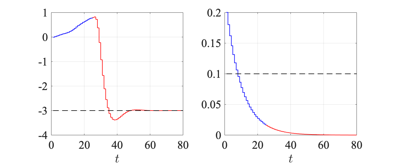
To illustrate our results, we consider the system (1) where
| (13) |
One can verify that the above is uncontrollable. We let and generate online input-output trajectories , where is sampled uniformly from for all such that is persistently exciting of order . At time , given , we obtain the input by solving (12), where , , , , and for all . Fig. 1 shows that, although the system contains an uncontrollable output (right), online DeePC still ensures that the controllable output (left) tracks the reference value as desired.
III-B Identification of homogeneous multi-agent systems
An important paradigm in formation control is the homogeneous multi-agent system, i.e., a network of agents with the same LTI dynamics [24, 25]. In such a system, each agent can measure the state of agent in a local coordinate system if is an edge of a directed graph , which is composed of nodes and edges. The dynamics of this multi-agent system is given by (1) with
| (14) |
where and describe the input-state dynamics of an individual agent. Each row of matrix is indexed by a directed edge, i.e., an edge with a head and a tail, in graph : the -th entry in each row is “” if node is the head of the corresponding edge, “” if it is the tail, and “” otherwise. We assume that is a non-zero matrix and is controllable.
If at least one non-zero entry in matrix is known, then system matrices in (14) can be computed using the following Markov parameters [26, Sec. 3.4.4]
| (15) | ||||
In particular, let denote the -th block of . If we know (the case of is similar), then (15) implies . For example, if , then (15) says . Hence given the Markov parameters (15) and that , we know is “” if , “” if , and “0” otherwise. Further, and is the unique solution to the following linear equations111Since is controllable, matrix has full column rank and (16) has a unique solution.
| (16) |
Therefore, given at least one non-zero entry in matrix , in order to compute the system matrices in (14), it suffices to know the Markov parameters (15). These parameters can be computed using Corollary 2 via a data-driven simulation procedure [3, 7] (see Appendix for details).
In numerical simulations, we consider the homogeneous multi-agent system used in [24, Example 3], discretized with a sampling time of 0.1s such that the system dynamics is given by (14) where
In addition, we let , where is the vector of all ’s.
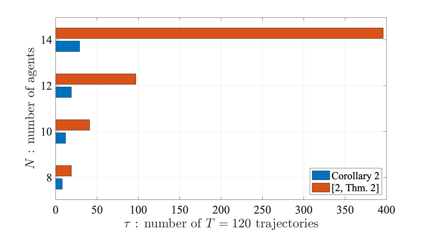
We compare Corollary 2 against the results in [2, Thm. 2] in terms of the least amount of input-output data needed to compute matrices in (14). In particular, since matrix has spectrum radius , we use use input-output trajectories with relatively short length to avoid numerical instability [2]. The entries in are sampled uniformly from . Using Corollary 2, the data-driven simulation procedure requires to be collectively persistently exciting of order . In other words, matrix (8) with has full row rank, hence it must have at least as many columns as rows, i.e.,
In comparison, if we use [2, Thm. 2] instead of Corollary 2, we need to be collectively persistently exciting of order (see [2, Sec. IV-A]). In other words, matrix (8) with has full row rank, which implies
In Fig. 2, we show the minimum number of input-output trajectories required to compute matrices in (14) in numerical simulations. The results tightly match the aforementioned two lower bounds, and the number of trajectories required by Corollary 2 is one order of magnitude less than that of [2, Thm. 1] when .
IV Conclusions
We introduced an extension of Willems’ fundamental lemma by relaxing the controllability and persistency of excitation assumptions. We demonstrate the usefulness of our results in the context of DeePC and identification of homogeneous multi-agent system. Future directions include generalizations to noisy data and nonlinear systems.
Appendix
Proof of Theorem 1
We start by proving the first statement using a double inclusion argument. Using an argument similar to (5), one can directly show that the left hand side of (9) is included in its right hand side. To show the other direction, we show that the left kernel of matrix
| (17) |
is orthogonal to . To this end, let
| (18) |
be an arbitrary row vector in the left kernel of matrix (17), where . Since , using [20, Def. 3.3.2], we know there exists such that
| (19) |
The above equation implies that and for all and Therefore in order to show the left kernel of matrix (17) is orthogonal to , it suffices to show the following
| (20a) | ||||
| (20b) | ||||
| (20c) | ||||
In order to prove (20a), we let be such that and equals
for . Since is in the left kernel of matrix (17), using (1) one can verify that are in the left kernel of
| (21) |
Let and in (19), we have . Hence
| (22) |
for some vector . Since row vectors are in the left kernel of matrix (21), equation (22) implies that is in the left kernel of matrix
| (23) |
Since is collectively persistently exciting of order , matrix (23) has full row rank. Therefore
| (24) |
Observe that the last entries of are given by , hence equation (24) implies that . Then the last entries of are given by . Since and , equation (24) also implies that . By repeating similar induction we can prove that (20a) holds.
Next, since (20a) holds, the first entries in are
By combining this with (24) we get that
| (25) |
Since , considering in (25) implies that . Substitute this back into (25) and considering implies that . By repeating a similar reasoning for we can prove that (20b) holds.
Further, by using (19) and (20b) we can show that for all . Combining this together with the fact that row vector (18) is in the left kernel of matrix (17) and that (20a) also holds, it follows that,
Since for by assumption, we conclude that (20c) holds.
We now prove the second statement. Given the input, state, and output trajectories in (3), suppose (7) holds. Let
| (26) | ||||
Then from (9) we know satisfies (10), and one can verify that is indeed an input-state-output trajectory of system (1).
Conversely, let be an input-state-output trajectory of system (1) with . Then there exists
| (27) |
such that and
| (28) |
where
| (29) | ||||
Further, using the Cayley-Hamilton theorem one can show that for any . Hence (27) implies
| (30) |
Since , the first statement of Theorem 1 implies that there exists such that
| (31) |
Notice that
| (32) |
for . Substituting (30), (31) and (32) into (28) gives (7), thus completing the proof. ∎
Proof of Corollary 1
First, let be such that is an input-state-output trajectory generated by the system (1). Then (5) holds for all . Hence is an input-state-output trajectory generated by system (1) that satisfies (5). From the second statement in Theorem 1 we know that is parameterizable by . Second, if is parameterizable by , then one can verify that it is indeed an input-output trajectory generated by the system (1) by constructing a length- state trajectory similar to the one in (26). ∎
Markov parameters computation in Section III-B
Let be input-output trajectories of the system described by (14), such that inputs are collectively persistently exciting of order . Let . Since in (14) is controllable, one can verify that , regardless of the values of . Using Corollary 2 we know that there exists a matrix such that,
| (33) | ||||
for all , where and is given by (15); also see [7, Sec. 4.5] for details. Next, given , we can compute by first solving the first equations in (33) for matrix , then substituting the solution into the last equations in (33). By repeating this process for we obtain Markov parameters (15). Using Kalman decomposition one can verify that Markov parameters of system (14) are the same as those of a reduced order controllable and observable system with state dimension less than . Hence matrix obtained this way is unique; see [7, Prop. 1].
References
- [1] J. C. Willems, P. Rapisarda, I. Markovsky, and B. L. De Moor, “A note on persistency of excitation,” Syst. Control Lett., vol. 54, no. 4, pp. 325–329, 2005.
- [2] H. J. van Waarde, C. De Persis, M. K. Camlibel, and P. Tesi, “Willems’ fundamental lemma for state-space systems and its extension to multiple datasets,” IEEE Control Syst. Lett., vol. 4, no. 3, pp. 602–607, 2020.
- [3] I. Markovsky, J. C. Willems, P. Rapisarda, and B. L. De Moor, “Algorithms for deterministic balanced subspace identification,” Automatica, vol. 41, no. 5, pp. 755–766, 2005.
- [4] T. Katayama, Subspace methods for system identification. Springer Science & Business Media, 2006.
- [5] I. Markovsky, “From data to models,” in Low-Rank Approximation. Springer, 2019, pp. 37–70.
- [6] J. Berberich and F. Allgöwer, “A trajectory-based framework for data-driven system analysis and control,” in Eur. Control Conf. IEEE, 2020, pp. 1365–1370.
- [7] I. Markovsky and P. Rapisarda, “Data-driven simulation and control,” Int. J. Control, vol. 81, no. 12, pp. 1946–1959, 2008.
- [8] T. Maupong and P. Rapisarda, “Data-driven control: A behavioral approach,” Syst. Control Lett., vol. 101, pp. 37–43, 2017.
- [9] A. Bisoffi, C. De Persis, and P. Tesi, “Data-based guarantees of set invariance properties,” arXiv preprint arXiv:1911.12293[eecs.SY], 2019.
- [10] C. De Persis and P. Tesi, “Formulas for data-driven control: Stabilization, optimality, and robustness,” IEEE Trans. Autom. Control, vol. 65, no. 3, pp. 909–924, 2019.
- [11] L. Huang, J. Coulson, J. Lygeros, and F. Dörfler, “Data-enabled predictive control for grid-connected power converters,” in IEEE Conf. Decision Control. IEEE, 2019, pp. 8130–8135.
- [12] J. Coulson, J. Lygeros, and F. Dörfler, “Data-enabled predictive control: In the shallows of the deepc,” in Eur. Control Conf. IEEE, 2019, pp. 307–312.
- [13] D. Alpago, F. Dörfler, and J. Lygeros, “An extended Kalman filter for data-enabled predictive control,” IEEE Control Systems Letters, vol. 4, no. 4, pp. 994–999, 2020.
- [14] J. Berberich, J. Koehler, M. A. Muller, and F. Allgower, “Data-driven model predictive control with stability and robustness guarantees,” IEEE Transactions on Automatic Control, pp. 1–1, 2020.
- [15] A. Allibhoy and J. Cortés, “Data-based receding horizon control of linear network systems,” arXiv preprint arXiv:2003.09813, 2020.
- [16] M. Yin, A. Iannelli, and R. S. Smith, “Maximum likelihood estimation in data-driven modeling and control,” arXiv preprint arXiv:2011.00925 [eess.SY], 2020.
- [17] F. Fabiani and P. J. Goulart, “The optimal transport paradigm enables data compression in data-driven robust control,” arXiv preprint arXiv:2005.09393 [eess.SY], 2020.
- [18] V. K. Mishra, I. Markovsky, and B. Grossmann, “Data-driven tests for controllability,” IEEE Control Syst. Lett., vol. 5, no. 2, pp. 517–522, 2020.
- [19] I. Markovsky and F. Dörfler, “Identifiability in the behavioral setting,” Dept. ELEC, Vrije Universiteit Brussel, Tech. Rep., 2020.
- [20] R. A. Horn and C. R. Johnson, Matrix analysis. Cambridge university press, 2012.
- [21] D. Q. Mayne, J. B. Rawlings, C. V. Rao, and P. O. Scokaert, “Constrained model predictive control: Stability and optimality,” Automatica, vol. 36, no. 6, pp. 789–814, 2000.
- [22] D. Q. Mayne, “Model predictive control: Recent developments and future promise,” Automatica, vol. 50, no. 12, pp. 2967–2986, 2014.
- [23] H. Mayeda and T. Yamada, “Strong structural controllability,” SIAM Journal on Control and Optimization, vol. 17, no. 1, pp. 123–138, 1979.
- [24] G. Wen, Z. Duan, W. Ren, and G. Chen, “Distributed consensus of multi-agent systems with general linear node dynamics and intermittent communications,” Int. J. Robust. Nonlinear Control, vol. 24, no. 16, pp. 2438–2457, 2014.
- [25] K.-K. Oh, M.-C. Park, and H.-S. Ahn, “A survey of multi-agent formation control,” Automatica, vol. 53, pp. 424–440, 2015.
- [26] M. Verhaegen and V. Verdult, Filtering and system identification: a least squares approach. Cambridge University Press, 2007.