On Boundaries of -neighbourhoods
of Planar Sets, Part I: Singularities

Jeroen S.W. Lamb Jeroen S.W. Lamb
Department of Mathematics
Imperial College London
180 Queen's Gate, London SW7 2AZ, United Kingdom [email protected] , Martin Rasmussen Martin Rasmussen
Department of Mathematics
Imperial College London
180 Queen's Gate, London SW7 2AZ, United Kingdom [email protected] and Kalle Timperi Kalle Timperi
Department of Mathematics
Imperial College London
180 Queen's Gate, London SW7 2AZ, United Kingdom [email protected]

Abstract.

We study geometric and topological properties of singularities on the boundaries of $\varepsilon$ -neighbourhoods $E_{\varepsilon}=\{x\in\mathbb{R}^{2}\,:\,\textrm{dist}(x,E)\leq\varepsilon\}$ of planar sets $E\subset\mathbb{R}^{2}$ . We develop a novel technique for analysing the boundary and obtain, for a compact set $E$ and $\varepsilon>0$ , a classification of singularities (i.e. non-smooth points) on $\partial E_{\varepsilon}$ into eight categories. We also show that the set of singularities is either countable or the disjoint union of a countable set and a closed, totally disconnected, nowhere dense set.

2020 Mathematics Subject Classification:

51F30; 57K20, 54C50, 51M15, 58C06

1. Introduction

1.1. Motivation

For a given set $E\subset\mathbb{R}^{d}$ and radius $\varepsilon>0$ , the (closed) $\varepsilon$ -neighbourhood of $E$ is the set

(1.1)

E_{\varepsilon}:=\overline{B_{\varepsilon}(E)}:=\overline{\bigcup_{x\in E}B_{\varepsilon}(x)},

where the overline denotes closure and $B_{\varepsilon}(\cdot)$ is an open ball of radius $\varepsilon$ in the Euclidean metric. The sets $E_{\varepsilon}$ are also known in the literature as tubular neighbourhoods [15], collars [24] or parallel sets [27, 33]. The boundary $\partial E_{\varepsilon}$ is a subset of the set $\partial E_{<\varepsilon}:=\partial\left(\bigcup_{x\in E}B_{\varepsilon}(x)\right)$ , which is sometimes referred to as the $\varepsilon$ -boundary [14] or $\varepsilon$ -level set [23] of $E$ .

The central question addressed in this paper concerns the geometric and topological properties of such sets $E_{\varepsilon}$ , with a focus on properties of its boundary $\partial E_{\varepsilon}$ . This is not only a very natural and fundamental question in (Euclidean) geometry, but it is also relevant in specific settings where $\varepsilon$ -neighbourhoods naturally arise. For instance, we are motivated by the classification and bifurcation of minimal invariant sets in random dynamical systems with bounded noise [21], but $\varepsilon$ -neighbourhoods also naturally feature for instance in control theory [9].

Notwithstanding significant theoretical progress on the properties of $\varepsilon$ -neighbourhoods during the last decades, the geometric classification of possible boundaries $\partial E_{\varepsilon}$ has remained open, even in dimension two.

1.2. Main results

Refer to caption — Figure 1. Schematic illustration of Theorem 1. The grey area represents the $\varepsilon$ -neighbourhood $E_{\varepsilon}$ , the white area the complement $\mathbb{R}^{2}\setminus E_{\varepsilon}$ . Every boundary point $x\in\partial E_{\varepsilon}$ either is a smooth point or belongs to exactly one of eight categories of singularities. At a *wedge* (S1) the one-sided tangents form an angle $0<\theta<\pi$ . A *sharp singularity* (S2) and a *sharp-sharp singularity* (S3) can be thought of as extremal cases of a wedge, with $\theta=0$ . A *shallow singularity* (S4) and a *shallow-shallow singularity* (S5) have a well-defined tangent, but they are accumulation points (from one or two directions, respectively) of sequences of increasingly obtuse wedges (black dots). A *chain singularity* (S6), a *chain-chain singularity* (S7) and a *sharp-chain singularity* (S8) share the geometric property of being accumulation points of sequences of increasingly acute wedges (black dots). This turns out to be equivalent (see Proposition 4.5) to the topological property of being the limit with respect to Hausdorff distance (see Definition 3.2) of a sequence of disjoint connected components of the complement $E_{\varepsilon}^{c}$ . See also Figure 9.

Our main achievement is the development of a novel technique for analysing geometric properties of the boundary $\partial E_{\varepsilon}$ , enabling a local representation for the boundary around every boundary point $x\in\partial E_{\varepsilon}$ via graphs of Lipschitz continuous functions. We employ this representation to obtain a classification of points on the boundary of $\varepsilon$ -neighbourhoods of compact planar sets.

Our first main result establishes that for any compact set $E\in\mathbb{R}^{2}$ and $\varepsilon>0$ , each boundary point $x\in\partial E_{\varepsilon}$ is either a smooth point (in the sense that, in a neighbourhood of $x$ , $\partial E_{\varepsilon}$ is a $C^{1}$ -curve) or falls into exactly one of eight distinct categories of singularities.

Theorem 1.

Let $E\subset\mathbb{R}^{2}$ be compact, $\varepsilon>0$ , and let $x\in\partial E_{\varepsilon}$ be a boundary point of $E_{\varepsilon}$ that is not smooth. Then $x$ belongs to precisely one of the following eight categories:

(S1)	wedge,	(S5)	shallow-shallow singularity,
(S2)	sharp singularity,	(S6)	chain singularity,
(S3)	sharp-sharp singularity,	(S7)	chain-chain singularity,
(S4)	shallow singularity,	(S8)	sharp-chain singularity.

Definition 4.1 contains a rigorous definition of these categories, but for indicative sketches of the singularity types, see Figure 1.

The proof of Theorem 1 is based on the construction of a local boundary representation, given in Proposition 3.5, that allows us to treat small parts of the boundary $\partial E_{\varepsilon}$ as finite unions of graphs of continuous functions. This representation in turn relies on a local contribution property, Proposition 3.1, which states that the geometry of the boundary near each boundary point $x\in\partial E_{\varepsilon}$ essentially depends on contributions from points $y\in E$ in at most two directions.

Using these same ingredients, we establish our second main result regarding the cardinality of the different types of singularities.

Theorem 2.

For any compact set $E\subset\mathbb{R}^{2}$ , the number of wedges (S1), sharp singularities (S2, S3 and S8), one-sided shallow singularities (S4) and chain singularities (S6) on $\partial E_{\varepsilon}$ is at most countably infinite.

In addition, we present examples which illustrate that the sets of shallow-shallow singularities (S5) and chain-chain singularities (S7) may be uncountable on $\partial E_{\varepsilon}$ , see Examples 5.5 and 5.7. We refer to the union of categories S6, S7 and S8 as chain singularities and denote the set of chain singularities on $\partial E_{\varepsilon}$ by $\mathcal{C}(\partial E_{\varepsilon})$ . Even though the set of chain-chain singularities (S7) may in general be uncountable and can have a positive Hausdorff measure on the boundary $\partial E_{\varepsilon}$ , our third main result establishes the fact that $\mathcal{C}(\partial E_{\varepsilon})$ is closed and totally disconnected.

Theorem 3.

For any compact set $E\subset\mathbb{R}^{2}$ and $\varepsilon>0$ , the set $\mathcal{C}(\partial E_{\varepsilon})$ of chain singularities is closed and totally disconnected.

As a corollary, Theorem 3 implies that $\mathcal{C}(\partial E_{\varepsilon})$ is nowhere dense on $\partial E_{\varepsilon}$ , and is hence small in the topological sense.

1.3. Context

Building on the topological groundwork of [4] and [7], our paper constitutes a first step in the analysis of the local geometry and topological properties of the boundary $\partial E_{\varepsilon}$ , with a particular focus on singularities. A main difference with the majority of the existing literature on boundaries of $\varepsilon$ -neighourhoods in this direction [4, 7, 14, 15, 28, 29, 33], is that we do not require (implicit) conditions on $\varepsilon$ .

-neighbourhoods arise in many branches of mathematics, ranging from convex analysis and manifold theory [24] to fractal geometry [18] and stochastic processes [20]. In the latter, so-called Wiener sausages represent smoothed-out counterparts of Brownian motion trajectories [10, 16, 25, 26], with applications in theoretical physics [17, 22, 32]. The interplay between the surface area and volume of $\varepsilon$ -neighbourhoods [27, 33] and different notions of dimension [18], as well as the dependence of the manifold structure of the boundary $\partial E_{\varepsilon}$ on the radius $\varepsilon$ [13, 14, 15, 28, 29] have all received considerable attention during the last decades. In particular, Rataj and collaborators [25, 26, 27, 28, 29] have advanced the understanding in recent years.

The study of $\varepsilon$ -neigbourhoods $E_{\varepsilon}$ and their boundaries dates back at least to the 1940s and Paul Erdős's remarks [11] regarding their measurability. Following Brown's (1972) initial topological observations [7], Ferry (1976) showed that $\varepsilon$ -boundaries are $(d-1)$ -manifolds in dimensions $d=2,3$ for almost all $\varepsilon>0$ , but that this fails for $d\geq 4$ [14]. Setting up the problem in a more extensive theoretical framework, Fu (1985) used the semiconcavity of the distance function $x\mapsto\operatorname{dist}(x,E)$ to show that the complement $\mathbb{R}^{d}\setminus E_{\varepsilon}$ is a set of positive reach, as defined by Federer (1959) [13, 15]. This allowed him to show that for an arbitrary compact set $E\subset\mathbb{R}^{d}$ in dimension $d\leq 3$ there exists an exceptional set $R_{E}\subset\mathbb{R}_{+}$ of Lebesgue measure $0$ , with the property that the boundaries $\partial E_{\varepsilon}$ are Lipschitz manifolds whenever $\varepsilon\notin R_{E}$ . Rataj and Zajíček (2020) has improved further on these results by providing optimal conditions on the smallness of the set $R_{E}$ [29].

1.4. Outlook

Our novel technique also allows for the analysis of global topological and regularity properties of the boundary $\partial E_{\varepsilon}$ . This is the topic of the sequel (part II) to this paper. While our results for the moment concern the properties boundaries of $\varepsilon$ -neighbourhoods of only planar sets $E\subset\mathbb{R}^{2}$ , our techniques appear well-suited for obtaining local and global properties of boundaries of $\varepsilon$ -neighbourhoods also in higher dimensions. It would be of particular interest to consider the above-mentioned results of Ferry [14] from this complementary point of view.

Finally, the current paper and its sequel have arisen from our interest in bifurcations of minimal invariant sets of random dynamical systems with bounded noise, which naturally appear as dynamically defined $\varepsilon$ -neighbourhoods. In this context, the aim is to develop a theory which allows for the characterisations of topological and/or geometric changes of such sets in parametrised families. The results in this paper provide a characterisation of boundaries at fixed values of parameters (including $\varepsilon$ ), which is a first step towards more general results concerning the classifications of qualitative changes of minimal invariant sets in (generic) parametrised families of random dynamical systems with bounded noise.

1.5. Structure of the paper

The rest of this paper is structured as follows. In Section 2 we lay out the basic conceptual framework and terminology that will be used throughout the paper. Section 2.2 contains a concise introduction to the notions and basic properties of contributors (Definition 2.1) and outward directions (Definition 2.4) and their relationship with tangential properties of the boundary $\partial E_{\varepsilon}$ .

In Section 3 we shed light on local properties of boundary points $x\in\partial E_{\varepsilon}$ in small neighbourhoods $\overline{B_{r}(x)}$ . The key result is Proposition 3.1, which states that for $E\subset\mathbb{R}^{2}$ the boundary geometry near each $x\in\partial E_{\varepsilon}$ is defined solely by those $y\in\partial E$ that lie near the extremal contributors (Definition 2.6) of $x$ . Building on this insight and a related approximation scheme (Definition 3.3) we show that the boundary can be represented locally by a finite union of continuous graphs (Proposition 3.5). This representation plays a pivotal role in the proofs of subsequent. Section 3.3 contains an analysis of the topological and geometric structure of the complement $E_{\varepsilon}^{c}$ near smooth points, wedges (S1) and shallow singularities (S4–S5).

Sections 4 and 5 contain the main results of this paper. We lay out the different types of singularities encountered on the boundary $\partial E_{\varepsilon}$ (Definition 4.1) and show how various types of singularities can be characterised in terms of the local topological structure of the complement $E_{\varepsilon}^{c}$ and the geometric properties of the boundary $\partial E_{\varepsilon}$ (Propositions 4.2 and 4.5, Corollary 4.3). Section 4 culminates with the proof of our first main result (Theorem 1), by establishing the fact that the classification of singularities, provided in Definition 4.1, defines a partition of $\partial E_{\varepsilon}$ .

Finally, in Section 5.1 cardinalities of the sets of different types of singularities are discussed, and the paper concludes with the proofs of the other two main results, Theorems 2 and 3.

2. -neighbourhoods

The object of our study is the $\varepsilon$ -neighbourhood $E_{\varepsilon}=\overline{B_{\varepsilon}(E)}$ of a closed subset $E\subset\mathbb{R}^{d}$ . The main results of this paper concern $\varepsilon$ -neighbourhoods of planar sets $E\subset\mathbb{R}^{2}$ , but we provide the basic definitions in a more general $d$ -dimensional setting. Throughout the paper we make the assumption that the underlying set $E\subset\mathbb{R}^{d}$ is closed¹¹1Note that this is not an actual restriction, since $\mathrm{dist}(x,E)=\mathrm{dist}(x,\overline{E})$ for all $x\in\mathbb{R}^{d}$ and $E\subset\mathbb{R}^{d}$ . and $\varepsilon>0$ . Many of the results require the stronger assumption of compactness; where necessary, this will be explicitly stated in the formulation of each result.

The most immediate observation regarding the structure of the set $E_{\varepsilon}$ is that each $x\in\partial E_{\varepsilon}$ necessarily lies on the boundary of a closed ball $\overline{B_{\varepsilon}(y)}$ of radius $\varepsilon$ , centered at some $y\in\partial E$ . On the other hand, for each $x\in\partial E_{\varepsilon}$ there may exist more than one $y\in\partial E$ with $\left\lVert y-x\right\rVert=\varepsilon$ . These considerations motivate the following definition.

Definition 2.1 (Contributor).

Let $E\subset\mathbb{R}^{d}$ be closed. For each $x\in\partial E_{\varepsilon}$ we define the set of contributors as the collection

\Pi_{E}(x):=\big{\{}y\in\partial E\,\,:\,\,\left\lVert y-x\right\rVert=\varepsilon\big{\}}.

Boundary points $x\in\partial E_{\varepsilon}$ with only one contributor constitute the set

\mathrm{Unp_{\varepsilon}}(E):=\big{\{}x\in\partial E_{\varepsilon}\,:\,\Pi_{E}(x)=\{y\}\,\,\textrm{for some}\,\,y\in\partial E\big{\}},

where $\mathrm{Unp}$ stands for 'unique nearest point', see [13, Definition 4.1].

The set of contributors $\Pi_{E}(x)$ consists of those points on $\partial E$ that minimise the distance from $\partial E$ to $x$ . Hence $\Pi_{E}$ can be interpreted as a restriction onto $\partial E_{\varepsilon}$ of the (set-valued) projection $\mathrm{proj}_{E}:\mathbb{R}^{2}\to E$ given by $\mathrm{proj}_{E}(x):=\{y\in E\,:\,\left\lVert y-x\right\rVert=\mathrm{dist}(x,E)\}$ . In terms of our classification of boundary points (see Definition 4.1 and Figures 1 and 9) the set $\mathrm{Unp_{\varepsilon}}(E)$ consists of smooth points and shallow singularities (S4–S5).

Definition 2.2 (Smooth point, singularity).

We call a boundary point $x\in\mathrm{Unp_{\varepsilon}}(E)$ smooth, if there exists a neighbourhood $B_{r}(x)$ for which $\partial E_{\varepsilon}\cap B_{r}(x)\subset\mathrm{Unp_{\varepsilon}}(E)$ . If $x$ is not smooth, we call it a singularity and write $x\in S(E_{\varepsilon})$ .

The rationale for Definition 2.2 stems from the fact that any smooth $x\in\partial E_{\varepsilon}$ in terms of Definition 2.2 turns out to be equivalent to $x$ having a neighbourhood $B_{r}(x)$ in which the boundary is a $C^{1}$ -smooth curve, see Proposition 4.6.

2.1. Tangents via Outward Directions

Our first objective is to shed light on the tangential properties of individual boundary points $x\in\partial E_{\varepsilon}$ . Acknowledging that classical tangents do not necessarily exist everywhere on the boundary, we adopt a set-valued definition of tangency which allows for several tangential directions to exist at each point. Our definition is a restriction of [13, Definition 4.3] to the boundary $\partial E_{\varepsilon}$ .

Definition 2.3 (Tangent set).

Let $E\subset\mathbb{R}^{d}$ be closed and $x\in\partial E_{\varepsilon}$ . We define the set $T_{x}(E_{\varepsilon})$ of unit tangent vectors of $E_{\varepsilon}$ at $x$ as all those points $v\in S^{d-1}$ for which there exists a sequence $(x_{n})_{n=1}^{\infty}\subset\partial E$ of boundary points satisfying $x_{n}\to x$ and

\frac{x_{n}-x}{\left\lVert x_{n}-x\right\rVert}\rightarrow v,\quad\textrm{as }\,n\to\infty.

In order to study the existence of tangential directions at boundary points $x\in\partial E_{\varepsilon}$ , we relate the set $T_{x}(E_{\varepsilon})$ to what we call outward directions. Intuitively, the set of outward directions at each $x$ contains the angles at which $x$ can be approached from the complement $E_{\varepsilon}^{c}:=\mathbb{R}^{d}\setminus E_{\varepsilon}$ . It turns out that for an $\varepsilon$ -neighbourhood $E_{\varepsilon}$ , the extremal values of these angles coincide with the tangential directions as defined in Definition 2.3. Hence the existence of tangents at each $x\in\partial E_{\varepsilon}$ hinges on the existence and properties of corresponding outward directions, which turn out to be easier to study due to their geometric relationship with the contributors $y\in\Pi_{E}(x)$ .

We define outward directions as points on the unit sphere $S^{d-1}\subset\mathbb{R}^{d}$ but think of them rather as directional vectors in the ambient space $\mathbb{R}^{d}$ , since we want to operate with them using the Euclidean scalar product $\langle\cdot,\cdot\rangle\,:\,\mathbb{R}^{d}\times\mathbb{R}^{d}\to\mathbb{R}$ .

Definition 2.4 (Outward direction).

Let $E\subset\mathbb{R}^{d}$ be closed. We say that a point $\xi\in S^{d-1}$ is an outward direction from $E_{\varepsilon}$ at a boundary point $x\in\partial E_{\varepsilon}$ , if there exists a sequence $(x_{n})_{n=1}^{\infty}\subset E_{\varepsilon}^{c}$ , for which $x_{n}\to x$ and

\xi_{n}:=\frac{x_{n}-x}{\left\lVert x_{n}-x\right\rVert}\longrightarrow\xi\in S^{d-1}\subset\mathbb{R}^{d},

as $n\to\infty$ . We denote by $\Xi_{x}(E_{\varepsilon})$ the set of outward directions from $E_{\varepsilon}$ at $x$ .

Remark 2.5.

The concept of outward directions is a variation of the well-known contingent cone, introduced by Bouligand (see for instance [2, 3, 31] and Bouligand's original work [5, 6]). For a boundary point $x\in\partial E_{\varepsilon}$ the contingent cone (Bouligand cone) $C_{x}(E_{\varepsilon})$ consists of those vectors $v\in\mathbb{R}^{d}$ , for which there exist sequences $(h_{n})_{n=1}^{\infty}\subset\mathbb{R}_{+}$ and $(v_{n})_{n=1}^{\infty}\subset\mathbb{R}^{d}$ for which $x+h_{n}v_{n}\in E_{\varepsilon}$ for all $n\in\mathbb{N}$ and

h_{n}\to 0,\quad\textrm{and}\quad v_{n}\to v

as $n\to\infty$ . If instead of the outward directions $\Xi_{x}(E_{\varepsilon})$ one considers at each $x\in\partial E_{\varepsilon}$ the contingent cone $C_{x}(E_{\varepsilon}^{c})$ for the complement $E_{\varepsilon}^{c}$ , it follows that $\mathcal{W}_{x}(E_{\varepsilon})=C_{x}(E_{\varepsilon}^{c})$ , where

\mathcal{W}_{x}(E_{\varepsilon}):=\left\{s\xi\,:\,\xi\in\Xi_{x}(E_{\varepsilon}),\,s\geq 0\right\}

denotes the outward cone at $x$ . We do not make use of this correspondence, but for further information on tangent cones, see for instance [8, 30].

For each $x\in\partial E_{\varepsilon}$ we single out those outward directions $\xi\in\Xi_{x}(E_{\varepsilon})$ that are perpendicular to some contributor $y\in\Pi_{E}(x)$ —we call these the extremal outward directions and extremal contributors (see Figure 2). Definition 2.6 below emphasises this geometric relationship, while Proposition 2.12 in the next subsection confirms that extremal outward directions can equivalently be defined via the topological property of constituting the boundary of the set of outward directions $\Xi_{x}(E_{\varepsilon})$ .

Definition 2.6 (Extremal contributor, extremal outward direction).

Let $E\subset\mathbb{R}^{d}$ be closed and $x\in\partial E_{\varepsilon}$ . If an outward direction $\xi\in\Xi_{x}(E_{\varepsilon})$ and a contributor $y\in\Pi_{E}(x)$ satisfy

\langle y-x,\xi\rangle=0,

we call $\xi$ an extremal outward direction and $y$ an extremal contributor at $x$ . For each $x\in\partial E_{\varepsilon}$ , we write $\Xi_{x}^{\mathrm{ext}}(E_{\varepsilon})$ and $\Pi_{E}^{\mathrm{ext}}(x)$ for the sets of extremal outward directions and extremal contributors, respectively.

The precise correspondence between extremal contributors, extremal outward directions, and tangential directions at each $x\in\partial E_{\varepsilon}$ is presented in Section 2.2, where we collect in one place all the basic results that we need in the remainder of the paper. The existence of outward directions at each $x\in\partial E_{\varepsilon}$ is established in Proposition 2.7 and their geometric relationship with the contributors is explored in Lemma 2.10 and Proposition 2.12. The coincidence of the set of tangential directions $T_{x}(E)$ with the set of extremal outward directions $\Xi_{x}^{\mathrm{ext}}(E_{\varepsilon})$ is established in Proposition 2.14.

2.2. Properties of Contributors and Outward Directions

We collect here the basic properties of contributors and outward directions that we need in our analysis of the boundary $\partial E_{\varepsilon}$ . The proofs make repeated use of convergent subsequences and scalar products and are rather elementary, although at places somewhat tedious. As before, the set $E\subset\mathbb{R}^{d}$ is assumed to be closed, and $\varepsilon>0$ .

Proposition 2.7 (The set of outward directions is non-empty and closed).

Let $E\subset\mathbb{R}^{d}$ be closed and $x\in\partial E_{\varepsilon}$ . Then the set $\Xi_{x}(E_{\varepsilon})$ of outward directions is non-empty and closed.

Proof.

Let $x\in\partial E_{\varepsilon}$ and choose some sequence $(x_{n})_{n=1}^{\infty}$ in $E_{\varepsilon}^{c}$ with $x_{n}\to x$ . This implies $x_{n}\neq x$ for all $n\in\mathbb{N}$ since $E_{\varepsilon}$ is closed. One may hence define a sequence $(\xi_{n})_{n=1}^{\infty}$ in $S^{1}$ by setting $\xi_{n}:=(x_{n}-x)/\left\lVert x_{n}-x\right\rVert$ for all $n\in\mathbb{N}$ . The compactness of $S^{1}$ implies that $(\xi_{n})_{n=1}^{\infty}$ has a convergent subsequence, the limit of which is an element in $\Xi_{x}(E_{\varepsilon})$ .

To show that $\Xi_{x}(E_{\varepsilon})$ is closed, let $\xi\in S^{d-1}$ and assume there exists a sequence $\left(\xi^{(n)}\right)_{n=1}^{\infty}\subset\Xi_{x}(E_{\varepsilon})$ with $\xi^{(n)}\to\xi$ as $n\to\infty$ . One needs to show that this implies $\xi\in\Xi_{x}(E_{\varepsilon})$ . We first use Definition 2.4 to identify each of the directions $\xi^{(n)}$ with a convergent sequence in $E_{\varepsilon}^{c}$ , and then apply a kind of diagonalisation argument in order to construct a new sequence $(z_{n})_{n=1}^{\infty}$ in $E_{\varepsilon}^{c}$ with $(z_{n}-x)/\left\lVert z_{n}-x\right\rVert\to\xi$ .

Without loss of generality, let $\left\lVert\xi^{(n)}-\xi\right\rVert\leq\frac{1}{n}$ for all $n\in\mathbb{N}$ . Now, for each $n\in\mathbb{N}$ one can choose a sequence $\big{(}x_{k}^{(n)}\big{)}_{k=1}^{\infty}\subset E_{\varepsilon}^{c}$ with $x_{k}^{(n)}\to x$ and

\xi_{k}^{(n)}:=\frac{x_{k}^{(n)}-x}{\big{\|}x_{k}^{(n)}-x\big{\|}}\longrightarrow\xi^{(n)},\quad\textrm{as }\,k\to\infty.

Consequently there exists for each $n\in\mathbb{N}$ some $K(n)\in\mathbb{N}$ , for which $\big{\|}x_{k}^{(n)}-x\big{\|}\leq 1/n$ and $\big{\|}\xi_{k}^{(n)}-\xi^{(n)}\big{\|}\leq 1/n$ for all $k\geq K(n)$ . Using these indices one can define a new sequence by setting $z_{n}:=x_{K(n)}^{(n)}$ for each $n\in\mathbb{N}$ . Accordingly

\left\lVert z_{n}-x\right\rVert=\big{\|}x_{K(n)}^{(n)}-x\big{\|}\leq\frac{1}{n}

so that $z_{n}\to x$ . Furthermore, writing $\xi_{n}^{z}:=(z_{n}-x)/\left\lVert z_{n}-x\right\rVert=\xi_{K(n)}^{(n)}$ , we have

\displaystyle\left\lVert\xi_{n}^{z}-\xi\right\rVert

\displaystyle\leq\big{\|}\xi_{K(n)}^{(n)}-\xi^{(n)}\big{\|}+\big{\|}\xi^{(n)}-\xi\big{\|}\leq\frac{2}{n}\longrightarrow 0

as $n\to\infty$ . Thus $\xi$ is the outward direction corresponding to the sequence $\left(z_{n}\right)_{n=1}^{\infty}$ , which implies $\xi\in\Xi_{x}(E_{\varepsilon})$ , as required. ∎

Despite their simplicity, the following Lemmas 2.8 and 2.9 regarding contributors are a key ingredient in many of the subsequent proofs.

Lemma 2.8 (Convergence of contributors).

Let $E\in\mathbb{R}^{d}$ be compact, let $(x_{n})_{n=1}^{\infty}\subset E_{\varepsilon}$ with $x_{n}\to x\in\partial E_{\varepsilon}$ , and $(y_{n})_{n=1}^{\infty}\subset E$ with $x_{n}\in\overline{B_{\varepsilon}(y_{n})}$ for all $n\in\mathbb{N}$ . Then there exists some $y\in\Pi_{E}(x)$ and a convergent subsequence $(y_{n_{k}})_{k=1}^{\infty}$ , for which $y_{n_{k}}\to y$ as $k\to\infty$ .

Proof.

Due to compactness of $E$ , there exists a convergent subsequence $(y_{n_{k}})_{k=1}^{\infty}$ with $y_{n_{k}}\to y\in E$ as $k\to\infty$ . For each $k\in\mathbb{N}$ ,

\left\lVert y-x\right\rVert\leq\left\lVert y-y_{n_{k}}\right\rVert+\left\lVert y_{n_{k}}-x_{n_{k}}\right\rVert+\left\lVert x_{n_{k}}-x\right\rVert,

which implies $\left\lVert y-x\right\rVert\leq\varepsilon$ , since $x_{n_{k}}\to x$ , $y_{n_{k}}\to y$ , and $\lim_{k\to\infty}\left\lVert y_{n_{k}}-x_{n_{k}}\right\rVert\leq\varepsilon$ . On the other hand $\left\lVert y-x\right\rVert\geq\textrm{dist}(x,E)=\varepsilon$ . Hence $\left\lVert y-x\right\rVert=\varepsilon$ , so that $y\in\Pi_{E}(x)$ . ∎

Lemma 2.9 (Tails of directed sequences).

Let $E\subset\mathbb{R}^{d}$ be compact, $(x_{n})_{n=1}^{\infty}\subset\mathbb{R}^{d}$ with $x_{n}\to x\in\partial E_{\varepsilon}$ and $x_{n}\neq x$ for all $n\in\mathbb{N}$ , and assume

v_{n}:=\frac{x_{n}-x}{\left\lVert x_{n}-x\right\rVert}\longrightarrow v,\quad\textrm{as }\,n\to\infty.

(i)

If $\langle y-x,v\rangle>0$ for some $y\in\Pi_{E}(x)$ , then there exists some $N\in\mathbb{N}$ , for which $x_{n}\in B_{\varepsilon}(y)$ for all $n\geq N$ .
(ii)

If $\langle y-x,v\rangle<0$ for all $y\in\Pi_{E}(x)$ , then there exists some $N\in\mathbb{N}$ , for which $x_{n}\in E_{\varepsilon}^{c}$ for all $n\geq N$ .

Proof.

(i) Assume $\langle y-x,v\rangle=p>0$ for some $y\in\Pi_{E}(x)$ . Then $\langle y-x,v_{n}\rangle\to p$ due to the continuity of the scalar product. Hence there exists some $N\in\mathbb{N}$ for which $\langle y-x,v_{n}\rangle>\frac{1}{2}p$ and $\left\lVert x_{n}-x\right\rVert<p$ , whenever $n\geq N$ . This implies

\left\lVert x_{n}-x\right\rVert<p<2\langle y-x,v_{n}\rangle

for all $n\geq N$ so that

	$\displaystyle\left\lVert y-x_{n}\right\rVert^{2}$	$\displaystyle=\left\lVert(y-x)-(x_{n}-x)\right\rVert^{2}$
		$\displaystyle=\varepsilon^{2}+\left\lVert x_{n}-x\right\rVert\left(\left\lVert x_{n}-x\right\rVert-2\langle y-x,v_{n}\rangle\right)<\varepsilon^{2}.$

(ii) Assume to the contrary that there exists a subsequence $(x_{n_{k}})_{k=1}^{\infty}\subset E_{\varepsilon}$ . Then for each $k$ there exists some $y_{k}\in E$ for which $\left\lVert x_{n_{k}}-y_{k}\right\rVert\leq\varepsilon$ . Since $E$ is compact, Lemma 2.8 implies the existence of some $y^{*}\in\Pi_{E}(x)$ for which $y_{k}\to y^{*}$ (if necessary, one can switch to a further convergent subsequence). By assumption $y^{*}\in\Pi_{E}(x)$ implies $\langle y^{*}-x,v\rangle<0$ . Due to the continuity of the scalar product there exists some $q>0$ and $K\in\mathbb{N}$ , for which $\langle y_{k}-x_{n_{k}},v_{n_{k}}\rangle\leq-\frac{1}{2}q$ and $\left\lVert x_{n_{k}}-x\right\rVert<q$ , whenever $k\geq K$ . Then

\left\lVert x_{n_{k}}-x\right\rVert+2\langle y_{k}-x_{n_{k}},v_{n_{k}}\rangle<0

for all $k\geq K$ , and applying the triangle-inequality with respect to the points $x_{n_{k}}$ yields

\displaystyle\left\lVert y_{k}-x\right\rVert^{2}

\displaystyle\leq\varepsilon^{2}+\left\lVert x_{n_{k}}-x\right\rVert\left(\left\lVert x_{n_{k}}-x\right\rVert+2\langle y_{k}-x_{n_{k}},v_{n_{k}}\rangle\right)<\varepsilon^{2}.

This implies the contradiction $x\in\textrm{int}(E_{\varepsilon})$ . ∎

Lemma 2.10 below provides a partial characterisation of outward directions $\Xi_{x}(E_{\varepsilon})$ in terms of the contributors $\Pi_{E}(x)$ . Geometrically it implies that outward directions point away from the vectors $y-x$ for all $y\in\Pi_{E}(x)$ , see Figure 2.

Lemma 2.10 (Orientation of outward directions relative to contributors).

Let $E\subset\mathbb{R}^{d}$ be compact, $x\in\partial E_{\varepsilon}$ and $\xi\in S^{d-1}$ . Then

(i)

if $\xi\in\Xi_{x}(E_{\varepsilon})$ , then $\langle y-x,\xi\rangle\leq 0$ for all $y\in\Pi_{E}(x)$ ,
(ii)

if $\langle y-x,\xi\rangle<0$ for all $y\in\Pi_{E}(x)$ , then $\xi\in\Xi_{x}(E_{\varepsilon})$ .

Proof.

(i) If $\xi\in\Xi_{x}(E_{\varepsilon})$ , there exists a sequence $(x_{n})_{n=1}^{\infty}\subset E_{\varepsilon}^{c}$ , for which $x_{n}\to x$ and $\xi_{n}:=(x_{n}-x)/\left\lVert x_{n}-x\right\rVert\to\xi$ as $n\to\infty$ . Assume contrary to the claim tha there exists some $y\in\Pi_{E}(x)$ with $\langle y-x,\xi\rangle>0$ . Substituting $v_{n}=\xi_{n}$ and $v=\xi$ in Lemma 2.9 (i) implies the existence of some $N\in\mathbb{N}$ for which $x_{n}\in\textrm{int}(E_{\varepsilon})$ for all $n\geq N$ . This contradicts the claim.

(ii) Write $\xi_{n}=\frac{1}{n}\xi$ , and define $x_{n}:=x+\xi_{n}$ , so that $(x_{n}-x)/\left\lVert x_{n}-x\right\rVert=\xi$ for all $n\in\mathbb{N}$ . Substituting $v:=\xi$ and $v_{n}:=\xi_{n}$ in Lemma 2.9 (ii) implies the existence of some $N\in\mathbb{N}$ for which $x_{n}\in E_{\varepsilon}^{c}$ for all $n\geq N$ . The sequence $(x_{n})_{n=N}^{\infty}$ now defines the outward direction $\xi\in\Xi_{x}(E_{\varepsilon})$ . ∎

Note that assuming the weaker condition $\langle y-x,\xi\rangle\leq 0$ for all contributors $y\in\Pi_{E}(x)$ is not sufficient in Lemma 2.10 (ii). For example, let $E:=[2,3]\times\{0,1\}$ and consider the set $E_{\varepsilon}$ with $\varepsilon=1/2$ . Then $x:=(3,1/2)\in\partial E_{\varepsilon}$ with $\Pi(x)=\{(3,0),(3,1)\}$ and has only one outward direction $\xi=(1,0)$ . Here also $\eta:=(-1,0)$ satisfies $\langle y-x,\eta\rangle=0$ for $y\in\{(3,0),(3,1)\}$ , and yet $\eta\notin\Xi_{x}(E_{\varepsilon})$ . This example illustrates the difference between $\partial E_{\varepsilon}$ and the $\varepsilon$ -boundary $\partial E_{<\varepsilon}$ (see Section 1.1), since here $\partial E_{<\varepsilon}\setminus\partial E_{\varepsilon}=(2,3)\times\{1/2\}\subset\mathrm{int}\,E_{\varepsilon}$ . See also [27, Example 2.1].

In order to describe the geometry of the sets of outward directions $\Xi_{x}(E_{\varepsilon})$ on the circle $S^{1}$ , we introduce the concept of a geodesic arc-segment. Intuitively, a geodesic arc-segment is the shortest curve on $S^{1}$ that connects two points $v,w\in S^{1}$ .

Definition 2.11 (Geodesic arc-segment).

Let $v,w\in S^{1}\subset\mathbb{R}^{2}$ and let

(2.1)

[v,w]_{S^{1}}:=\left\{u\in S^{1}\,:\,u=av+bw\,\textrm{ for some }a,b\geq 0\right\}.

For $w\neq-v$ , the set $[v,w]_{S^{1}}$ defines a geodesic arc-segment between $v$ and $w$ . We also define the corresponding open geodesic arc-segment $(v,w)_{S^{1}}\subset S^{1}$ as

(2.2)

(v,w)_{S^{1}}:=[v,w]_{S^{1}}\setminus\{v,w\}.

We use the notations $[v,w]_{S^{1}}$ and $(v,w)_{S^{1}}$ in accordance with (2.1) and (2.2) also for the cases $v=w$ and $v=-w$ , even though the corresponding sets in these cases are not arc-segments.

Unlike the previous results in this section, we formulate and prove the statements in Proposition 2.12 and Lemma 2.13 below only for the two-dimensional case. Note also that Proposition 2.12 is formulated for a compact set $E\subset\mathbb{R}^{2}$ , but essentially the same proof works for any closed set $E$ due to the local nature of the result.

Proposition 2.12 (Structure of sets of outward directions).

Let $E\subset\mathbb{R}^{2}$ be compact and $x\in\partial E_{\varepsilon}$ . Then the set of outward directions $\Xi_{x}(E_{\varepsilon})$ satisfies the following.

(i)

If $x\in\mathrm{Unp_{\varepsilon}}(E)$ , then $\Xi_{x}(E_{\varepsilon})=\left\{\xi\in S^{1}\,:\,\langle y-x,\xi\rangle\leq 0\right\}$ ;
(ii)

If $x\notin\mathrm{Unp_{\varepsilon}}(E)$ , then $\Xi_{x}(E_{\varepsilon})=[\xi_{1},\xi_{2}]_{S^{1}}$ , where $\xi_{1},\xi_{2}$ are the only extremal outward directions at $x$ , possibly satisfying $\xi_{1}=\xi_{2}$ .

Proof.

(i) Since $\Pi_{E}(x)=\{y\}$ , Lemma 2.10 (ii) implies

X:=\{\xi\in S^{1}\,:\,\langle y-x,\xi\rangle<0\}\subset\Xi_{x}(E_{\varepsilon}).

Then $\partial_{S^{1}}X=\{\xi\in S^{1}\,:\,\langle y-x,\xi\rangle=0\}$ due to continuity of the scalar product, and Lemmas 2.7 and 2.10 (i) imply $\overline{X}=\Xi_{x}(E_{\varepsilon})$ , as claimed.

(ii) Assume then that $\Pi_{E}(x)$ contains at least two points. We assert that

(a)

if $\xi,\eta\subset\Xi_{x}(E_{\varepsilon})$ and $\gamma\in(\xi,\eta)_{S^{1}}$ , then $\langle y-x,\gamma\rangle<0$ for all $y\in\Pi_{E}(x)$ ,
(b)

$\xi\in\textrm{int}_{S^{1}}\Xi_{x}(E_{\varepsilon})$ if and only if $\langle y-x,\xi\rangle<0$ for all $y\in\Pi_{E}(x)$ ,
(c)

$\Xi_{x}(E_{\varepsilon})=[\xi_{1},\xi_{2}]_{S^{1}}$ .

(a) If $\Xi_{x}(E_{\varepsilon})=\{\xi\}$ or $\Xi_{x}(E_{\varepsilon})=\{\xi,-\xi\}$ for some $\xi\in S^{1}$ , the claim is true since $(\xi,\xi)_{S^{1}}=(\xi,-\xi)_{S^{1}}=\varnothing$ .

Let $\xi,\eta\in\Xi_{x}(E_{\varepsilon})$ with $\eta\notin\{\xi,-\xi\}$ and define a parametrised curve $\gamma:[0,1]\to S^{1}$ by

\gamma(t):=\frac{t\eta+(1-t)\xi}{\left\lVert t\eta+(1-t)\xi\right\rVert}.

Clearly $\gamma(0)=\xi,\gamma(1)=\eta$ , and $\gamma((0,1))=(\xi,\eta)_{S^{1}}$ . For each $y\in\Pi_{E}(x)$ , consider the scalar product

(2.3)		$\displaystyle P_{y}(t):=\langle y-x,t\eta+(1-t)\xi\rangle$	$\displaystyle=t\langle y-x,\eta\rangle+(1-t)\langle y-x,\xi\rangle$
(2.4)			$\displaystyle=\langle y-x,\xi\rangle+t\langle y-x,\eta-\xi\rangle.$

We show that $P_{y}(t)<0$ for every $y\in\Pi_{E}(x)$ and all $t\in(0,1)$ . We have $P_{y}(t)\leq 0$ for all $t\in[0,1]$ and all $y\in\Pi_{E}(x)$ , since Lemma 2.10 (i) guarantees

\langle y-x,\eta\rangle\leq 0\quad\textrm{and}\quad\langle y-x,\xi\rangle\leq 0

for all $y\in\Pi_{E}(x)$ . For $t\in(0,1)$ , equation (2.3) implies $P_{y}(t)<0$ when $\langle y-x,\xi\rangle<0$ . On the other hand, if $\langle y-x,\xi\rangle=0$ , equation (2.4) implies

t\langle y-x,\eta-\xi\rangle=P_{y}(t)\leq 0.

Hence the inequality $P_{y}(t)<0$ holds if and only if $\eta\notin\{\xi,-\xi\}$ . This shows that $P_{y}(t)<0$ for arbitrary $y\in\Pi_{E}(x)$ , whenever $t\in(0,1)$ .

(b) If $\xi\in S^{1}$ satisfies $\langle y-x,\xi\rangle<0$ for all $y\in\Pi_{E}(x)$ , then there exists some $n\in\mathbb{N}$ for which $\langle y-x,\xi\rangle<-1/n$ for all $y\in\Pi_{E}(x)$ . To show this, assume to the contrary that for each $n\in\mathbb{N}$ there exists some $y_{n}\in\Pi_{E}(x)$ for which

\langle y_{n}-x,\xi\rangle\geq-1/n.

Since $S^{1}$ is compact and $E$ is closed, there exists a convergent subsequence $(y_{n_{k}})_{k=1}^{\infty}\subset(y_{n})_{n=1}^{\infty}$ with $y_{n_{k}}\to y^{*}\in\Pi_{E}(x)$ . On the other hand, due to the continuity of the scalar product we have

\langle y^{*}-x,\xi\rangle=\lim_{k\to\infty}\langle y_{n_{k}}-x,\xi\rangle\geq 0,

which contradicts the assumption that $\langle y-x,\xi\rangle<0$ for all $y\in\Pi_{E}(x)$ .

Assume now that $\langle y-x,\xi\rangle<0$ for all $y\in\Pi_{E}(x)$ and that $n\in\mathbb{N}$ has been chosen so that $\langle y-x,\xi\rangle<-1/n$ for all $y\in\Pi_{E}(x)$ . The continuity of the scalar product implies that for some $\delta$ , depending on $n$ , one has $\left\langle y-x,\widehat{\xi}\right\rangle<0$ for all $\widehat{\xi}$ that satisfy $\left\lVert\widehat{\xi}-\xi\right\rVert<\delta$ . Hence $\xi$ has an open neighbourhood $B_{\delta}(\xi)$ satisfying $B_{\delta}(\xi)\cap S^{1}\subset\Xi_{x}(E_{\varepsilon})$ , which implies $\xi\in\textrm{int}_{S^{1}}\Xi_{x}(E_{\varepsilon})$ .

For the other direction, assume $\xi\in\textrm{int}_{S^{1}}\Xi_{x}(E_{\varepsilon})$ . Then there exist $\eta_{1},\eta_{2}\in\Xi_{x}(E_{\varepsilon})$ , for which $\xi\in(\eta_{1},\eta_{2})_{S^{1}}\subset\textrm{int}_{S^{1}}\Xi_{x}(E_{\varepsilon})$ . Step (a) consequently implies $\langle y-x,\xi\rangle<0$ for all $y\in\Pi_{E}(x)$ .

(c) It follows from steps (a) and (b) that $\textrm{int}_{S^{1}}\Xi_{x}(E_{\varepsilon})=(\xi_{1},\xi_{2})_{S^{1}}$ . This in turn implies $\Xi_{x}^{\mathrm{ext}}(E_{\varepsilon})=\{\xi_{1},\xi_{2}\}$ , when $\textrm{int}_{S^{1}}\Xi_{x}(E_{\varepsilon})\neq\varnothing$ , and $\Xi_{x}(E_{\varepsilon})=\{\xi\}$ (singleton), when $\xi_{1}=\xi_{2}$ .∎

Proposition 2.12 thus gives the following geometric picture of the set of extremal outward directions. In the case of a sharp singularity (S2) or a chain singularity (S6) (see Figure 1 and Definition 4.1), the set of extremal outward directions is a singleton $\Xi_{x}^{\mathrm{ext}}(E_{\varepsilon})=\{\xi\}$ for some $\xi\in S^{1}$ . Otherwise $\Xi_{x}^{\mathrm{ext}}(E_{\varepsilon})$ contains two points, which may point directly away from each other or form an acute or obtuse angle.

Lemma 2.13 below summarises the limiting behaviour of outward directions $\xi_{n}$ and contributors $y_{n}$ of points $x_{n}$ that appear in convergent sequences on the $\varepsilon$ -neighbourhood boundary. In particular, Lemma 2.13 (ii)(a) establishes that for each $x\in\partial E_{\varepsilon}$ the set of tangent vectors $T_{x}(E_{\varepsilon})$ is a subset of the set $\Xi_{x}^{\mathrm{ext}}(E_{\varepsilon})$ of extremal outward directions. According to Proposition 2.14 these sets in fact coincide for all $x\in\partial E_{\varepsilon}$ .

Lemma 2.13 (Orientation in converging sequences of boundary points).

Let $E\subset\mathbb{R}^{2}$ be compact and let $x\in\partial E_{\varepsilon}$ . Furthermore, let $(x_{n})_{n=1}^{\infty}$ be a sequence on $\partial E_{\varepsilon}$ with $x_{n}\to x$ and define $\xi_{n}:=(x_{n}-x)/\left\lVert x_{n}-x\right\rVert$ for all $n\in\mathbb{N}$ . Then the following statements hold true:

(i)

The sequence $(\xi_{n})_{n=1}^{\infty}$ can be split into two disjoint, convergent subsequences $(\xi_{i,k})_{k=1}^{\infty}$ , where $i\in\{1,2\}$ and $\xi^{(i)}:=\lim_{k\to\infty}\xi_{i,k}\in\Xi_{x}^{\mathrm{ext}}(E_{\varepsilon})$ .
(ii)
If the limit $\xi:=\lim_{n\to\infty}\xi_{n}\in S^{1}$ exists, then
1. (a)
  
  every sequence $(y_{n})_{n=1}^{\infty}$ in $E$ with $y_{n}\in\Pi(x_{n})$ for all $n\in\mathbb{N}$ has a convergent subsequence $(y_{n_{k}})_{k=1}^{\infty}$ for which $y:=\lim_{k\to\infty}y_{n_{k}}\in\Pi_{E}^{\mathrm{ext}}(x)$ . Furthermore $\langle y-x,\xi\rangle=0$ and consequently $\xi\in\Xi_{x}^{\mathrm{ext}}(E_{\varepsilon})$ .
2. (b)
  
  every sequence $(\eta_{n})_{n=1}^{\infty}$ in $S^{1}$ with $\eta_{n}\in\Xi_{x_{n}}^{\mathrm{ext}}(E_{\varepsilon})$ for all $n\in\mathbb{N}$ satisfies
  
  $\lim_{n\to\infty}\left\lVert\langle\eta_{n},\xi\rangle\right\rVert=1.$

Proof.

(ii)(a) Due to Lemma 2.8, there exists some $y\in\Pi_{E}(x)$ and a convergent subsequence $(y_{n_{k}})_{k=1}^{\infty}\subset(y_{n})_{n=1}^{\infty}$ , for which $y_{n_{k}}\to y$ . We break the proof into three steps.

Step 1. $\langle y-x,\xi\rangle\leq 0$ : Assume contrary to the claim that $\langle y-x,\xi\rangle>0$ . Then substituting $x_{k}:=x_{n_{k}}$ and $v:=\xi$ in Lemma 2.9 (1) implies that for some $K\in\mathbb{N}$ we have $x_{n_{k}}\in\textrm{int}(E_{\varepsilon})$ for all $k\geq K$ . This contradicts the assumption $x_{n}\in\partial E_{\varepsilon}$ for all $n\in\mathbb{N}$ .

Step 2. $\langle y-x,\xi\rangle\geq 0$ : Assume contrary to the claim that $\langle y-x,\xi\rangle<0$ . The continuity of the scalar product then implies that there exists some $K\in\mathbb{N}$ for which $\left\lVert x_{n_{k}}-x\right\rVert+2\langle y_{n_{k}}-x_{n_{k}},\xi_{n_{k}}\rangle<0$ for all $k\geq K$ . Applying the triangle-inequality with respect to the points $x_{n_{k}}$ yields

\displaystyle\left\lVert y_{n_{k}}-x\right\rVert^{2}

\displaystyle=\varepsilon^{2}+\left\lVert x_{n_{k}}-x\right\rVert\left(\left\lVert x_{n_{k}}-x\right\rVert+2\langle y_{n_{k}}-x_{n_{k}},\xi_{n_{k}}\rangle\right)<\varepsilon^{2}

for all $k\geq K$ . This implies the contradiction $x\in\textrm{int}(E_{\varepsilon})$ .

Step 3. $\xi\in\Xi_{x}^{\mathrm{ext}}(E_{\varepsilon})$ : For each $n\in\mathbb{N}$ , write $r_{n}:=\left\lVert x_{n}-x\right\rVert$ . Since $(x_{n})_{n=1}^{\infty}\subset\partial E_{\varepsilon}$ there exists for each $n\in\mathbb{N}$ some $z_{n}\in B_{r_{n}^{2}}(x_{n})\cap E_{\varepsilon}^{c}$ . Then $\xi_{n}^{z}:=(z_{n}-x)/\left\lVert z_{n}-x\right\rVert\to\xi$ so that $\xi\in\Xi_{x}(E_{\varepsilon})$ . Steps 1. and 2. together imply $\langle y-x,\xi\rangle=0$ so that $\xi\in\Xi_{x}^{\mathrm{ext}}(E_{\varepsilon})$ (see Definition 2.6). This concludes the proof of (ii)(a).

(ii)(b) Assume contrary to the claim that there exists some $\delta>0$ and a subsequence $(\eta_{n_{k}})_{k=1}^{\infty}$ , for which $\left\lVert\langle\eta_{n_{k}},\xi\rangle\right\rVert<1-\delta$ for all $k\in\mathbb{N}$ . This implies that if $y_{k}\in\Pi_{E}^{\mathrm{ext}}(x_{n_{k}})$ with $\langle y_{k}-x_{n_{k}},\eta_{n_{k}}\rangle=0$ , there exists some $r>0$ , depending on $\delta$ , for which

(2.5)

\left\lVert\langle y_{k}-x_{n_{k}},\xi\rangle\right\rVert\geq r

for infinitely many $k\in\mathbb{N}$ . On the other hand property (ii)(a) implies the existence of a subsequence $(y_{k_{j}})_{j=1}^{\infty}$ for which the limit $y:=\lim_{j\to\infty}y_{k_{j}}\in\Pi_{E}^{\mathrm{ext}}(x)$ exists and satisfies $\langle y-x,\xi\rangle=0$ . Inequality (2.5) now leads to the contradiction

\left\lVert\langle y-x,\xi\rangle\right\rVert=\lim_{j\to\infty}\big{\|}\big{\langle}y_{k_{j}}-x_{n_{k_{j}}},\xi\big{\rangle}\big{\|}\geq r>0.

(i) According to (ii)(a) every convergent subsequence $(\xi_{n_{k}})_{k=1}^{\infty}$ satisfies $\xi_{n_{k}}\to\xi\in\Xi_{x}^{\mathrm{ext}}(E_{\varepsilon})$ as $k\to\infty$ . For $\Xi_{x}^{\mathrm{ext}}(E_{\varepsilon})=\{\xi\}$ (a singleton) this implies $\xi_{n}\to\xi$ and the claim follows. In case $\Xi_{x}^{\mathrm{ext}}(E_{\varepsilon})=\left\{\xi^{(1)},\xi^{(2)}\right\}$ for some $\xi^{(1)}\neq\xi^{(2)}$ , write $r=\big{\|}\xi^{(1)},\xi^{(2)}\big{\|}$ . The compactness of $\partial E_{\varepsilon}$ implies that there exists some $N\in\mathbb{N}$ , for which

\xi_{n}\in B_{r/3}\big{(}\xi^{(1)}\big{)}\cup B_{r/3}\big{(}\xi^{(2)}\big{)}

for all $n\geq N$ . For each $i\in\{1,2\}$ , define $N_{i}:=\left\{n\in\mathbb{N}\,:\,\xi_{n}\in B_{r/3}\left(\xi^{(i)}\right)\right\}$ . If $N_{i}$ is finite for some $i\in\{1,2\}$ , we have $\lim_{n\to\infty}\xi_{n}=\xi^{(j)}$ for $j\in\{1,2\}\setminus\{i\}$ and the claim follows. Otherwise the sequences $(\xi_{1,k})_{k\in N_{1}}$ and $(\xi_{2,k})_{k\in\mathbb{N}\setminus N_{1}}$ are disjoint and satisfy $\lim_{k\to\infty}\xi_{i,k}=\xi^{(i)}$ for $i\in\{1,2\}$ . ∎

Proposition 2.14 (Extremal outward directions coincide with tangents).

Let $E\subset\mathbb{R}^{2}$ be compact and let $x\in\partial E_{\varepsilon}$ . Then $T_{x}(E_{\varepsilon})=\Xi_{x}^{\mathrm{ext}}(E_{\varepsilon})$ .

Proof.

Lemma 2.13 (ii)(a) implies $T_{x}(E_{\varepsilon})\subset\Xi_{x}^{\mathrm{ext}}(E_{\varepsilon})$ , so we are left with proving the other direction. Assume $\xi\in\Xi_{x}^{\mathrm{ext}}(E_{\varepsilon})$ . Then there exists a sequence $(x_{n})_{n=1}^{\infty}\subset E_{\varepsilon}^{c}$ , for which

\frac{\varphi_{n}}{\left\lVert\varphi_{n}\right\rVert}:=\frac{x_{n}-x}{\left\lVert x_{n}-x\right\rVert}\longrightarrow\xi,

as $n\to\infty$ . Since $\xi$ is an extremal outward direction, there exists some extremal contributor $y\in\Pi_{E}^{\mathrm{ext}}(x)$ for which $\langle y-x,\xi\rangle=0$ . Let $\widehat{y}:=(y-x)/\left\lVert y-x\right\rVert=(y-x)/\varepsilon$ and define $H_{n}:=h_{n}\xi+r_{n}\widehat{y}$ , where

h_{n}:=\left\lVert\varphi_{n}\right\rVert\sqrt{1-\frac{\left\lVert\varphi_{n}\right\rVert^{2}}{4\varepsilon^{2}}},\quad\text{and}\quad r_{n}:=\frac{\left\lVert\varphi_{n}\right\rVert^{2}}{2\varepsilon}.

It follows from the orthogonality of $\xi$ and $\widehat{y}$ that $\left\lVert H_{n}\right\rVert=\left\lVert\varphi_{n}\right\rVert$ . Furthermore $x+H_{n}\in E_{\varepsilon}$ for all $n\in\mathbb{N}$ , since $\left\lVert\left(x+H_{n}\right)-y\right\rVert=\varepsilon$ . See figure 3.

Consider now the $\left\lVert\varphi_{n}\right\rVert$ -radius circle $\partial B_{\left\lVert\varphi_{n}\right\rVert}(x)$ centered at $x$ . The geodesic arc-segment (shortest path) on this circle that connects the points $x+H_{n}\in E_{\varepsilon}$ and $x+\varphi_{n}=x_{n}\in E_{\varepsilon}^{c}$ must necessarily contain a boundary point $z_{n}\in\partial B_{\left\lVert\varphi_{n}\right\rVert}(x)\cap\partial E_{\varepsilon}$ .

Let $\delta>0$ . Since $x_{n}\to x$ and $\varphi_{n}/\left\lVert\varphi_{n}\right\rVert\to\xi$ , there exists some $N\in\mathbb{N}$ for which

(2.6)

\left\lVert\varphi_{n}\right\rVert\leq\frac{\delta}{3}\quad\text{and}\quad\left\lVert\frac{\varphi_{n}}{\left\lVert\varphi_{n}\right\rVert}-\xi\right\rVert\leq\frac{\delta}{3}

whenever $n\geq N$ . Since

\displaystyle\left\lVert\frac{H_{n}}{\left\lVert H_{n}\right\rVert}-\xi\right\rVert^{2}

\displaystyle=2-\sqrt{4-\frac{\left\lVert\varphi_{n}\right\rVert^{2}}{\varepsilon^{2}}}\longrightarrow 0

as $\varphi_{n}\to 0$ , we can choose some $N^{*}\geq N$ for which the inequality $\left\lVert H_{n}/\left\lVert H_{n}\right\rVert-\xi\right\rVert\leq\delta/3$ as well as the estimates (2.6) hold for all $n\geq N^{*}$ . It follows from the definition of the points $z_{n}$ that $\left\lVert z_{n}-(x+\varphi_{n})\right\rVert\leq\left\lVert\varphi_{n}-H_{n}\right\rVert$ for all $n\in\mathbb{N}$ . This allows us to obtain the estimate

\displaystyle\left\lVert\frac{z_{n}-x}{\left\lVert z_{n}-x\right\rVert}-\xi\right\rVert

\displaystyle\leq\left\lVert\frac{H_{n}}{\left\lVert H_{n}\right\rVert}-\xi\right\rVert+2\left\lVert\frac{\varphi_{n}}{\left\lVert\varphi_{n}\right\rVert}-\xi\right\rVert\leq\delta,

which is valid for all $n\geq N^{*}$ . Since also $0<\left\lVert z_{n}-x\right\rVert=\left\lVert\varphi_{n}\right\rVert<\delta$ for all $n\geq N^{*}$ , we see that $\xi$ fulfils the requirements of Definition 2.3, so that $\xi\in T_{x}(E_{\varepsilon})$ . ∎

3. Local Structure of the Boundary

In this section we utilise the results obtained in Section 2 regarding outward directions and contributors in order to analyse the local properties of the boundary $\partial E_{\varepsilon}$ .

We begin by proving a local contribution property, Proposition 3.1, which intuitively states that in order to describe the local geometry of $\partial E_{\varepsilon}$ near a boundary point $x\in\partial E_{\varepsilon}$ it suffices to consider the geometry of $\partial E$ around the extremal contributors $y\in\Pi_{E}^{\mathrm{ext}}(x)$ .

In Section 3.2 we develop a method for approximating the set $E_{\varepsilon}$ with finite collections of balls $\{B_{\varepsilon}(d_{n})\,:\,d_{n}\in D^{n}\}$ that correspond to certain finite subsets $D^{n}\subset E$ . Combining this idea with Proposition 3.1 we proceed to show in Proposition 3.5 that local representations for the boundary $\partial E_{\varepsilon}$ may be obtained using finite collections of curves that can be represented as graphs of continuous functions on a compact interval.

As the first application of Proposition 3.5 we show in Lemma 3.8 that for every $x\in\mathrm{Unp_{\varepsilon}}(E)$ and every wedge (see Definition 4.1 and Figure 1) there exists a unique connected component $V$ of the complement $E_{\varepsilon}^{c}$ for which $x\in\partial V$ .

3.1. Local Contribution

Intuitively, one can give a crude approximation for the boundary around each $x\in\partial E_{\varepsilon}$ by considering the boundaries $\partial B_{\varepsilon}(y)$ centered at the contributors $y\in\Pi_{E}(x)$ , and zooming in on a suitably small neighbourhood $B_{r}(x)$ , in which

(3.1)

\partial E_{\varepsilon}\cap B_{r}(x)\approx\partial\left(\bigcup_{y\in\Pi_{E}(x)}B_{\varepsilon}(y)\right)\cap B_{r}(x).

However, inside any neighbourhood $B_{r}(x)$ the geometry of the $\varepsilon$ -neighbourhood $E_{\varepsilon}$ is not defined solely by the positions of the contributors $y\in\Pi_{E}(x)$ (see Figures 4 and 5). Hence one needs to consider at least all the contributors in some neighbourhood of the set of extremal contributors $\Pi_{E}^{\mathrm{ext}}(x)$ . Proposition 3.1 below confirms that this is indeed sufficient.

We introduce here the following notation for open $x$ -centered half-balls oriented in the direction of some $v\in S^{1}$ :

(3.2)

U_{r}(x,v):=\{z\in B_{r}(x)\,:\,\langle z-x,v\rangle>0\}.

Proposition 3.1 (Local contribution).

Let $E\subset\mathbb{R}^{2}$ and $x\in\partial E_{\varepsilon}$ with $\Xi_{x}^{\mathrm{ext}}(E_{\varepsilon})=\{\xi_{1},\xi_{2}\}$ , where we allow $\xi_{1}=\xi_{2}$ . Then for all $\delta>0$ there exists some $r>0$ such that given $z\in B_{r}(x)$ , we have $z\in E_{\varepsilon}$ if and only if either

(3.3)		$\displaystyle z$	$\displaystyle\notin\overline{U_{r}(x,\xi_{1})}\cup\overline{U_{r}(x,\xi_{2})},\mathrm{or}$
(3.4)		$\displaystyle z$	$\displaystyle\in\overline{B_{\varepsilon}\big{(}E\cap B_{\delta}(\Pi_{E}^{\mathrm{ext}}(x))\big{)}}.$

Proof.

Assume to the contrary that there exists some $\delta>0$ , for which the claim fails. This means that for all $r>0$ there exists some $z\in B_{r}(x)$ , for which either

(1)

$z\in E_{\varepsilon}$ and both (3.3) and (3.4) fail, or
(2)

$z\notin E_{\varepsilon}$ and one of the conditions (3.3) or (3.4) holds true.

This implies that there exists a sequence $(z_{k})_{k=1}^{\infty}$ with $z_{k}\in B_{1/k}(x)$ , for which either condition (1) or (2) holds true for $z=z_{k}$ for infinitely many indices $k\in\mathbb{N}$ . A corresponding subsequence $(z_{n})_{n=1}^{\infty}$ then satisfies $z_{n}\to x$ as $n\to\infty$ and either

(a)

for all $n\in\mathbb{N}$ $z_{n}\in E_{\varepsilon}$ while conditions (3.3) and (3.4) both fail for $z=z_{n}$ , or
(b)

for all $n\in\mathbb{N}$ $z_{n}\notin E_{\varepsilon}$ while either condition (3.3) or (3.4) holds true for $z=z_{n}$ .

We proceed by showing that both of these statements lead to a contradiction. In both cases one can assume, without loss of generality, the existence of the limit

v_{z}:=\lim_{n\to\infty}(z_{n}-x)/\left\lVert z_{n}-x\right\rVert.

Assume first that (a) holds true. This means that

(3.5)

z_{n}\in E_{\varepsilon}\cap\left(\overline{U_{1/n}(x,\xi_{1})}\cup\overline{U_{1/n}(x,\xi_{2})}\right)\quad\mathrm{and}\quad z_{n}\notin\overline{B_{\varepsilon}\big{(}E\cap B_{\delta}(\Pi_{E}^{\mathrm{ext}}(x))\big{)}}

for all $n\in\mathbb{N}$ . Since $z_{n}\in E_{\varepsilon}$ for all $n\in\mathbb{N}$ , one can choose a sequence $(y_{n})_{n=1}^{\infty}\subset E$ with $z_{n}\in\overline{B_{\varepsilon}(y_{n})}$ . In addition, since $z_{n}\to x$ , Lemma 2.8 guarantees the existence of a convergent subsequence $(y_{n_{k}})_{k=1}^{\infty}$ with the limit $\widehat{y}:=\lim_{k\to\infty}y_{n_{k}}\in\Pi_{E}(x)$ . Note that it follows from (3.5) that $y_{n}\notin B_{\delta}(\Pi_{E}^{\mathrm{ext}}(x))$ for all $n\in\mathbb{N}$ , which implies $\widehat{y}\notin\Pi_{E}^{\mathrm{ext}}(x)$ , and consequently $\Pi_{E}(x)\setminus\Pi_{E}^{\mathrm{ext}}(x)\neq\varnothing$ . This rules out the possibility $\xi_{1}=-\xi_{2}$ for the extremal outward directions $\xi_{1},\xi_{2}\in\Xi_{x}^{\mathrm{ext}}(E_{\varepsilon})$ , and therefore

(3.6)

\langle\xi_{1},\xi_{2}\rangle>-1.

The relations (3.5) guarantee that $z_{n_{k}}\notin B_{\varepsilon}(\Pi_{E}^{\mathrm{ext}}(x))$ , which together with Lemma 2.9 (i) implies $\langle y-x,v_{z}\rangle\leq 0$ for all extremal contributors $y\in\Pi_{E}^{\mathrm{ext}}(x)$ . Combined with the assumption that

z_{n_{k}}\in\overline{U_{1/k}(x,\xi_{1})}\cup\overline{U_{1/k}(x,\xi_{2})}

for all $k\in\mathbb{N}$ , this implies that $v_{z}\in[\xi_{1},\xi_{2}]_{S^{1}}=\Xi_{x}(E_{\varepsilon})$ (see Proposition 2.12), where $[\xi_{1},\xi_{2}]_{S^{1}}$ is a geodesic arc-segment due to (3.6). It follows that $\langle\widehat{y}-x,v_{z}\rangle<0$ , since $\widehat{y}\notin\Pi_{E}^{\mathrm{ext}}(x)$ . But now a computation analogous to that presented in the proof of Lemma 2.9 (ii) leads to the contradiction $\left\lVert\widehat{y}-x\right\rVert<\varepsilon$ .

Assume then that (b) holds true. Now $z_{n}\notin E_{\varepsilon}$ for all $n\in\mathbb{N}$ so that $v_{z}\in\Xi_{x}(E_{\varepsilon})$ . In addition, given that either (3.3) or (3.4) is satisfied for each $z_{n}$ and (3.4) implies $z_{n}\in E_{\varepsilon}$ , condition (3.3) necessarily holds true for all $z_{n}$ . Then $\xi_{1}\neq-\xi_{2}$ , since $\xi_{1}=-\xi_{2}$ leads to the contradiction

z_{n}\in B_{1/n}(x)\setminus\bigcup_{i\in\{1,2\}}\overline{U_{1/n}(x,\xi_{i})}=B_{1/n}(x)\setminus B_{1/n}(x)=\varnothing.

On the other hand, if $\xi_{1}\neq-\xi_{2}$ , Proposition 2.12 states that $v_{z}\in\Xi_{x}(E_{\varepsilon})$ can be written as a convex combination $v_{z}=a\xi_{1}+b\xi_{2}$ . Note that at least one of the coefficients $a,b$ must be strictly positive, since $v_{z}\in S^{1}$ . However, (3.3) implies $\langle z_{n}-x,\xi_{i}\rangle<0$ for $i\in\{1,2\}$ and all $n\in\mathbb{N}$ , which leads to the contradiction $\langle v_{z},\xi_{i}\rangle\leq 0$ for $i\in\{1,2\}$ . ∎

3.2. Approximating the Boundary with Continuous Graphs

In order to study the properties of the boundary $\partial E_{\varepsilon}$ , we develop a finite approximation scheme as a technical aid. The idea is to generate an expanding sequence $(D^{n})_{n=1}^{\infty}$ of finite subsets $D^{n}\subset E$ and consider their $\varepsilon$ -neighbourhoods $B_{\varepsilon}(D^{n})$ , whose boundaries approximate the actual boundary $\partial E_{\varepsilon}$ uniformly with respect to Hausdorff distance.

Definition 3.2 (Hausdorff distance).

The Hausdorff distance between $X,Y\subset\mathbb{R}^{d}$ is

\mathrm{dist}_{H}(X,Y):=\mathrm{inf}\big{\{}\delta>0\,:\,X\subset Y_{\delta}\,\,\textrm{and}\,\,Y\subset X_{\delta}\big{\}},

where $X_{\delta}:=\overline{\bigcup_{x\in X}B_{\delta}(x)}$ .

Let $E\subset\mathbb{R}^{2}$ be compact, $\varepsilon>0$ and $n_{0}\in\mathbb{N}$ with $n_{0}>\frac{\ln(4/\varepsilon)}{\ln 2}$ . Consider for natural numbers $n>n_{0}$ the partitions of $\mathbb{R}^{2}$ into squares

\mathcal{C}^{n}:=\left\{C_{k,\ell}^{n}:=\left[\frac{k}{2^{n}},\frac{k+1}{2^{n}}\right]\times\left[\frac{\ell}{2^{n}},\frac{\ell+1}{2^{n}}\right]:k,\ell\in\mathbb{Z}\right\}.

Due to the Axiom of Choice, there exists a non-decreasing sequence $D^{n_{0}}\subset D^{n_{0}+1}\subset\dots$ of subsets of $D^{n}$ of $\mathbb{R}^{2}$ such that

D^{n}\cap C_{k,\ell}^{n}=\left\{\begin{array}[]{c@{\quad\text{if}\,\,}l}\big{\{}d_{k,\ell}^{n}\big{\}}&E\cap C_{k,\ell}^{n}\not=\emptyset,\\ \emptyset&E\cap C_{k,\ell}^{n}=\emptyset,\end{array}\right.

where the points $d_{k,\ell}^{n}$ are chosen arbitrarily from $E\cap C_{k,\ell}^{n}$ . It is easy to verify that $E_{\varepsilon}=\bigcup_{n\geq n_{0}}B_{\varepsilon}(D^{n})$ and that the approximations converge to $E_{\varepsilon}$ in Hausdorff distance,

(3.7)

\lim_{n\to\infty}\operatorname{dist}_{H}\big{(}E_{\varepsilon},B_{\varepsilon}(D^{n})\big{)}=0\,.

Definition 3.3 (Finite approximating sets).

Let $E\subset\mathbb{R}^{2}$ be compact and let $(D^{n})_{n=1}^{\infty}$ be a sequence of subsets $D^{n}\subset E$ as described above. Then the sets $D^{n}$ are called finite approximating sets for the set $E$ .

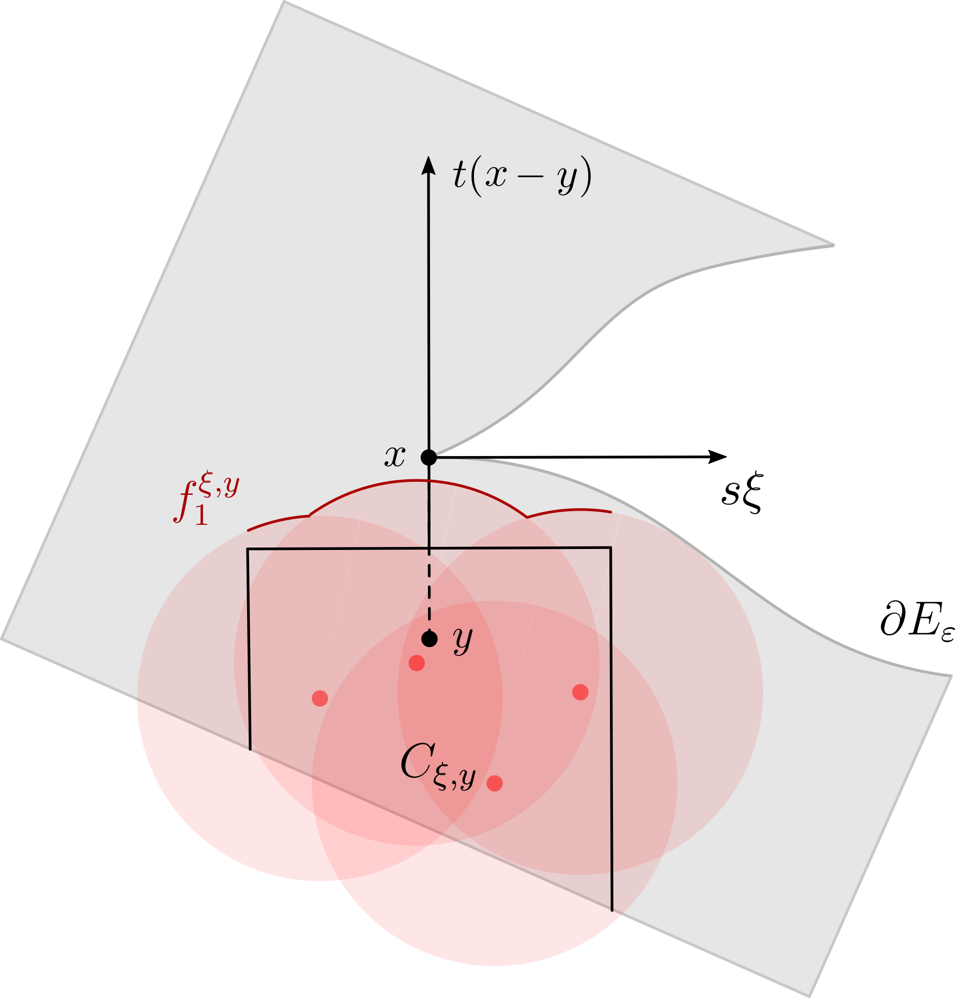
We now have the necessary ingredients in place for defining what we call local boundary representations near each boundary point $x\in\partial E_{\varepsilon}$ . The local contribution property, Proposition 3.1, implies that in order to describe the boundary $\partial E_{\varepsilon}$ near $x$ , one only needs to consider contributors $y\in E$ around the extremal contributors $y\in\Pi_{E}^{\mathrm{ext}}(x)$ . The extremal outward directions $\xi\in\Xi_{x}^{\mathrm{ext}}(E_{\varepsilon})$ together with their corresponding extremal contributors form extremal pairs $(\xi,y)$ that represent coordinate axes adapted to the orientation of the boundary near $x$ .

Definition 3.4 (Extremal pairs).

Let $E\subset\mathbb{R}^{d}$ be closed, let $x\in\partial E_{\varepsilon}$ and denote by $\Xi_{x}^{\mathrm{ext}}(E_{\varepsilon})$ and $\Pi_{E}^{\mathrm{ext}}(x)$ the sets of extremal outward directions and extremal contributors, respectively. We define the set of extremal pairs at $x$ as the collection

\mathcal{P}_{x}^{\mathrm{ext}}(E_{\varepsilon}):=\big{\{}(\xi,y)\in\Xi_{x}^{\mathrm{ext}}(E_{\varepsilon})\times\Pi_{E}^{\mathrm{ext}}(x)\,:\,\langle y-x,\xi\rangle=0\big{\}}.

One can thus choose a finite approximating sequence $D^{n}\subset E$ , interpret the boundaries $\partial B_{\varepsilon}(D^{n})$ near $x$ as graphs of continuous functions $f_{n}$ in the coordinate system $(\xi,y)\in\mathcal{P}_{x}^{\mathrm{ext}}(E_{\varepsilon})$ and obtain, as a uniform limit, a continuous function $f=\lim_{n\to\infty}f_{n}$ whose graph serves as a representation of a part of the boundary $\partial E_{\varepsilon}$ near $x$ . Using this construction for each extremal pair $(\xi,y)\in\mathcal{P}_{x}^{\mathrm{ext}}(E_{\varepsilon})$ one obtains a finite set of continuous graphs that give a complete representation of the boundary near $x$ .

We note that the proof of Proposition 3.5 below makes use of Lemma 3.7 which we have placed in the subsequent Section 3.3, together with other results on the geometry of the complement $E_{\varepsilon}^{c}$ .

Proposition 3.5 (Local boundary representation).

Let $E\subset\mathbb{R}^{2}$ be closed and let $x\in\partial E_{\varepsilon}$ . For each extremal pair $(\xi,y)\in\mathcal{P}_{x}^{\mathrm{ext}}(E_{\varepsilon})$ there exists a continuous function $f^{\xi,y}:[0,\varepsilon/2]\to\mathbb{R}$ and a corresponding function $g_{\xi,y}:[0,\varepsilon/2]\to\mathbb{R}^{2}$ , given by

(3.8)

g_{\xi,y}(s):=x+s\xi+f^{\xi,y}(s)(x-y),

so that the collection $\mathcal{G}(x):=\left\{g_{\xi,y}\,:\,(\xi,y)\in\mathcal{P}_{x}^{\mathrm{ext}}(E_{\varepsilon})\right\}$ satisfies

(3.9)

\partial E_{\varepsilon}\cap\overline{B_{r}(x)}=\bigcup_{(\xi,y)\in\mathcal{P}_{x}^{\mathrm{ext}}(E_{\varepsilon})}g_{\xi,y}\left(A_{\xi,y}\right)

for some $r>0$ and some closed $A_{\xi,y}\subset[0,\varepsilon/2]$ . We call the collection $\mathcal{G}(x)$ a local boundary representation (of radius $r$ ) at $x$ . For each extremal pair $(\xi,y)\in\mathcal{P}_{x}^{\mathrm{ext}}(E_{\varepsilon})$ the corresponding subset $A_{\xi,y}\subset[0,\varepsilon/2]$ is either

(a)

an interval $[0,s_{\xi,y}]$ for some $0<s_{\xi,y}\leq\varepsilon/2$ , or
(b)

a closed set whose complement in $[0,\varepsilon/2]$ contains a sequence of disjoint open intervals with $0$ as an accumulation point.

For wedges (type S1) and $x\in\mathrm{Unp_{\varepsilon}}(E)$ , case (a) above holds true for all $(\xi,y)\in\mathcal{P}_{x}^{\mathrm{ext}}(E_{\varepsilon})$ .

Proof.

Define for each extremal pair $(\xi,y)\in\mathcal{P}_{x}^{\mathrm{ext}}(E_{\varepsilon})$ the sets

	$\displaystyle C_{\xi,y}$	$\displaystyle:=\left\{x+s\xi+t(x-y)\,:\,(s,t)\in[-\varepsilon,\varepsilon]\times(-\infty,-\varepsilon/2]\right\},$
	$\displaystyle E_{\xi,y}$	$\displaystyle:=E\cap C_{\xi,y}.$

Consider a sequence $(D_{n})_{n=1}^{\infty}$ of finite approximating sets for the set $E$ (see Definition 3.3), and define $D_{n}^{\xi,y}:=E_{\xi,y}\cap D_{n}$ for each $n\in\mathbb{N}$ . Using the sets $D_{n}^{\xi,y}$ we define a sequence of functions $f_{n}^{\xi,y}:[-\varepsilon/2,\varepsilon/2]\to\mathbb{R}$ by setting

(3.10)

f_{n}^{\xi,y}(s):=\textrm{max}\left\{t\in\mathbb{R}\,:\,\mathrm{dist}\left(x+s\xi+t(x-y),D_{n}^{\xi,y}\right)\leq\varepsilon\right\},

where $\textrm{dist}\left(\cdot,D_{n}^{\xi,y}\right)$ denotes the Euclidean distance from the set $D_{n}^{\xi,y}$ . The maximum in (3.10) exists for all $s\in[-\varepsilon/2,\varepsilon/2]$ due to the compactness of $\overline{B_{\varepsilon}\big{(}D_{n}^{\xi,y}\big{)}}$ , which also implies that the functions $f_{n}^{\xi,y}$ are bounded for all $n\in\mathbb{N}$ . In addition, it follows from the definition of the values $f_{n}^{\xi,y}(s)$ that

x+s\xi+f_{n}^{\xi,y}(s)(x-y)\in\partial\overline{B_{\varepsilon}\big{(}D_{n}^{\xi,y}\big{)}}

for all $s\in[-\varepsilon/2,\varepsilon/2]$ . Since for each $n\in\mathbb{N}$ the boundary $\partial\overline{B_{\varepsilon}\big{(}D_{n}^{\xi,y}\big{)}}$ is composed of a finite collection of arc-segments, the corresponding functions $f_{n}^{\xi,y}$ are continuous.

It is easy to verify that the boundaries $\partial\overline{B_{\varepsilon}\left(D_{n}\right)}$ converge to the boundary $\partial E_{\varepsilon}$ uniformly in Hausdorff distance. Similarly the boundaries $\partial\overline{B_{\varepsilon}\big{(}D_{n}^{\xi,y}\big{)}}$ converge uniformly to the boundaries $\partial\overline{B_{\varepsilon}(E_{\xi,y})}$ . Hence $\left(f_{n}^{\xi,y}\right)_{n=1}^{\infty}$ is a uniformly convergent, monotonically increasing sequence of continuous functions on the compact interval $[-\varepsilon/2,\varepsilon/2]$ , which implies that the limiting function

(3.11)

f^{\xi,y}(s):=\lim_{n\to\infty}f_{n}^{\xi,y}(s)

is continuous. One can therefore define for each $(\xi,y)\in\mathcal{P}_{x}^{\mathrm{ext}}(E_{\varepsilon})$ a function $g_{\xi,y}:[0,\varepsilon/2]\to\mathbb{R}^{2}$ by

(3.12)

g_{\xi,y}(s):=x+s\xi+f^{\xi,y}(s)(x-y).

The remainder of the proof concerns the analysis of the relationship between the graphs $g_{\xi,y}([0,\varepsilon/2])$ and the boundary $\partial E_{\varepsilon}$ near the point $x$ , with the aim of identifying subsets $A_{\xi,y}\subset[0,\varepsilon/2]$ that satisfy (3.9).

Substituting $\delta=\varepsilon/2$ in Proposition 3.1 guarantees the existence of some $r>0$ , for which $z\in E_{\varepsilon}\cap B_{r}(x)$ if and only if either

\textrm{(i) }z\notin\overline{U_{r}(x,\xi)}\textrm{ for each }\xi\in\Xi_{x}^{\mathrm{ext}}(E_{\varepsilon}),\quad\textrm{or}\quad\textrm{(ii) }z\in\overline{B_{\varepsilon}\left(E\cap B_{\varepsilon/2}(\Pi_{E}^{\mathrm{ext}}(x))\right)}.

According to Proposition 2.14, the set of tangential directions $T_{x}(E_{\varepsilon})$ coincides with the set of extremal outward directions $\Xi_{x}^{\mathrm{ext}}(E_{\varepsilon})$ . This implies that condition (i) necessarily fails for all boundary points $z\in\partial E_{\varepsilon}\cap B_{r}(x)$ . Therefore condition (ii) holds true whenever $z\in\partial E_{\varepsilon}\cap B_{r}(x)$ , in which case $z\in\partial\overline{B_{\varepsilon}(E_{\xi,y})}$ for some $(\xi,y)\in\mathcal{P}_{x}^{\mathrm{ext}}(E_{\varepsilon})$ . Hence there exists some $s_{z}\in[0,\varepsilon/2]$ , for which $z=g_{\xi,y}(s_{z})$ . In other words, every boundary point $z\in\partial E_{\varepsilon}$ inside the neighbourhood $B_{r}(x)$ lies on one of the graphs $g_{\xi,y}([0,\varepsilon/2])$ with $(\xi,y)\in\mathcal{P}_{x}^{\mathrm{ext}}(E_{\varepsilon})$ .

It remains to be verified, for each $(\xi,y)\in\mathcal{P}_{x}^{\mathrm{ext}}(E_{\varepsilon})$ , which arguments $s\in[0,\varepsilon/2]$ satisfy $g_{\xi,y}(s)\in\partial E_{\varepsilon}\cap B_{r}(x)$ . We divide the rest of the proof into two cases, depending on whether or not there exist extremal contributors $y_{1},y_{2}\in\Pi_{E}^{\mathrm{ext}}(x)$ for which

(3.13)

y_{1}-x=-(y_{2}-x).

Condition (3.13) is schematically illustrated in Figure 9 (c) below.

(i) In case (3.13) is not satisfied by any $y_{1},y_{2}\in\Pi_{E}^{\mathrm{ext}}(x)$ , there is either only one contributor so that $x\in\mathrm{Unp_{\varepsilon}}(E)$ , or else $x$ is a wedge (see Definition 4.1). In both cases we have $\mathcal{P}_{x}^{\mathrm{ext}}(E_{\varepsilon})=\{(\xi_{1},y_{1}),(\xi_{2},y_{2})\}$ for some $\xi_{1},\xi_{2}\in\Xi_{\textrm{ext}}(x)$ and $y_{1},y_{2}\in\Pi_{E}^{\mathrm{ext}}(x)$ , where we allow for $y_{1}=y_{2}$ in case $x\in\mathrm{Unp_{\varepsilon}}(E)$ . It follows from Lemma 3.7 that for any outward directions $\eta_{1},\eta_{2}\in(\xi_{1},\xi_{2})_{S^{1}}$ there exists a neighbourhood $B_{\rho}(x)\subset B_{r}(x)$ in which the graphs of $g_{\xi_{1},y_{1}}$ and $g_{\xi_{2},y_{2}}$ are separated by the cone $V_{\rho}(x,\eta_{1},\eta_{2})$ . Hence

(3.14)

g_{\xi_{1},y_{1}}([0,\varepsilon/2])\cap g_{\xi_{2},y_{2}}([0,\varepsilon/2])\cap B_{\rho}(x)=\varnothing.

For $i\in\{1,2\}$ we define the upper bounds

s_{\xi_{i},y_{i}}:=\max\Big{\{}s\in[0,\varepsilon/2]\,:\,g_{\xi_{i},y_{i}}\left([0,s]\right)\in\overline{B_{\rho}(x)}\Big{\}}

and the corresponding sets $A_{\xi_{i},y_{i}}:=\left[0,s_{\xi_{i},y_{i}}\right]$ . It follows then from (3.14) and Proposition 3.1 that $g_{\xi_{i},y_{i}}(A_{\xi_{i},y_{i}})\subset\partial E_{\varepsilon}$ for $i\in\{1,2\}$ , which implies

\partial E_{\varepsilon}\cap\overline{B_{\rho}(x)}=\bigcup_{i\in\{1,2\}}g_{\xi_{i},y_{i}}\left(A_{\xi_{i},y_{i}}\right).

(ii) Assume then that (3.13) holds true for $y_{1},y_{2}\in\Pi_{E}^{\mathrm{ext}}(x)$ and consider some $\xi\in\Pi_{E}^{\mathrm{ext}}(x)$ . In this case the graphs $g_{\xi,y_{i}}([0,s])$ , $i\in\{1,2\}$ may generally intersect for arbitrarily small $s\in(0,\varepsilon/2]$ . Due to (3.13) one can write for $\{i,j\}=\{1,2\}$

	$\displaystyle g_{\xi,y_{i}}(s)$	$\displaystyle=x+s\xi+\left(f^{\xi,y_{j}}(s)-\alpha_{\xi}(s)\right)(x-y_{j})$
		$\displaystyle=g_{\xi,y_{j}}(s)-\alpha_{\xi}(s)(x-y_{j}),$

where $\alpha_{\xi}(s):=f^{\xi,y_{1}}(s)+f^{\xi,y_{2}}(s)$ . Hence it follows for $i\in\{1,2\}$ from Proposition 3.1 and the definitions of the functions $f_{n}^{\xi,y}$ and $f^{\xi,y}$ (see (3.10) and (3.11)) that

	$\displaystyle g_{\xi,y_{i}}(s)$	$\displaystyle\notin\partial E_{\varepsilon}\,\,\mathrm{whenever}\,\,\alpha_{\xi}(s)>0,\,\mathrm{and}$
	$\displaystyle g_{\xi,y_{i}}(s)$	$\displaystyle\in\partial E_{\varepsilon}\,\,\mathrm{whenever}\,\,\alpha_{\xi}(s)<0.$

For $\alpha_{\xi}(s)=0$ one has $g_{\xi,y_{1}}(s)=g_{\xi,y_{2}}(s)\in\partial E_{\varepsilon}$ if and only if there exists a sequence $(s_{n})_{n=1}^{\infty}$ with $s_{n}\to s$ , for which $\alpha_{\xi}(s_{n})<0$ for all $n\in\mathbb{N}$ . This follows from the fact that

\tau g_{\xi,y_{1}}(s)+(1-\tau)g_{\xi,y_{2}}(s)\in E_{\varepsilon}^{c}

whenever $s\in(0,r)$ , $\alpha_{\xi}(s)<0$ and $\tau\in(0,1)$ . Equation (3.9) is therefore satisfied for the neighbourhood $B_{r}(x)$ and the sets

A_{\xi,y_{i}}:=A_{\xi}:=\overline{\left\{s\in[0,r]\,:\,\alpha_{\xi}(s)<0\right\}}=\left\{s\in[0,r]\,:\,g_{\xi,y_{1}}(s),g_{\xi,y_{2}}(s)\in\partial E_{\varepsilon}\right\},

where $i\in\{1,2\}$ and $\xi\in\Xi_{x}^{\mathrm{ext}}(E_{\varepsilon})$ . Now either $[0,s_{\xi}]\subset A_{\xi}$ for some $s_{\xi}\in(0,r]$ or otherwise $[0,T]\setminus A_{\xi}\neq\varnothing$ for all $T>0$ . In any case $0$ is an accumulation point of $A_{\xi}$ , since $x\in\partial E_{\varepsilon}$ and $\xi\in T_{x}(E_{\varepsilon})$ (see Proposition 2.14). ∎

Consider a boundary point $x\in\partial E_{\varepsilon}$ and the corresponding local boundary representation $\mathcal{G}(x)$ with radius $r>0$ , and let $z\in\partial E_{\varepsilon}\cap B_{r}(x)$ with

z=g_{\xi,y}(s_{z})=x+s_{z}\xi+f^{\xi,y}(s_{z})(x-y)

for some $(\xi,y)\in\mathcal{P}_{x}^{\mathrm{ext}}(E_{\varepsilon})$ and $s_{z}\in[0,r]$ . The construction given in Proposition 3.5 guarantees that, when written in the $(\xi,y)$ -coordinates, the $\xi$ -coordinate $s_{w}$ of each contributor $w\in\Pi_{E}(z)$ satisfies $s_{w}\in[0,\varepsilon/2]$ . This implies a lower and upper bound for the local growth-rate of the function $f^{\xi,y}$ . Combining this observation with Proposition 2.14 allows us to deduce that the functions $f^{\xi,y}$ in (3.8) are in fact Lipschitz continuous on $[0,r]$ for all $(\xi,y)\in\mathcal{P}_{x}^{\mathrm{ext}}(E_{\varepsilon})$ , with a Lipschitz constant $K=1/\sqrt{3}\varepsilon$ .

Proposition 3.6 (Local boundary representation is Lipschitz).

Let $E\subset\mathbb{R}^{2}$ , let $x\in\partial E_{\varepsilon}$ and let $\mathcal{G}(x)$ be a local boundary representation at $x$ with radius $r>0$ . For each extremal pair $(\xi,y)\in\mathcal{P}_{x}^{\mathrm{ext}}(E_{\varepsilon})$ , the function $f^{\xi,y}$ in (3.8) is $1/\sqrt{3}\varepsilon$ -Lipschitz, and the function $g_{\xi,y}\in\mathcal{G}(x)$ is $2/\sqrt{3}$ -Lipschitz on the interval $[0,r]$ .

Proof.

In order to work in an orthonormal coordinate system, we define for all $(\xi,y)\in\mathcal{P}_{x}^{\mathrm{ext}}(E_{\varepsilon})$ the functions $h^{\xi,y}:[0,r]\to\mathbb{R}$ by setting $h^{\xi,y}(s):=\varepsilon f^{\xi,y}(s)$ so that

g_{\xi,y}(s)=x+s\xi+h^{\xi,y}(s)\varepsilon^{-1}(x-y)

for all $g_{\xi,y}\in\mathcal{G}(x)$ . We will show that the functions $h^{\xi,y}$ are $1/\sqrt{3}$ -Lipschitz, from which the claim follows.

Assume contrary to the claim that for some $(\xi,y)\in\mathcal{P}_{x}^{\mathrm{ext}}(E_{\varepsilon})$ there exist some $p>1/\sqrt{3}$ and $s,w\in[0,r]$ for which $|h^{\xi,y}(s)-h^{\xi,y}(w)|\geq p|s-w|$ . We present the argument for the case $w<s$ and $h^{\xi,y}(s)-h^{\xi,y}(w)\geq p(s-w)$ . Assuming $h^{\xi,y}(s)-h^{\xi,y}(w)\leq-p(s-w)$ leads to a contradiction through similar reasoning. Write $m:=(s+w)/2$ and define

(w_{1},s_{1}):=\left\{\begin{array}[]{c@{\quad\text{if}\,\,}l}(m,s)&h^{\xi,y}(s)-h^{\xi,y}(m)>p(s-m),\\ (w,m)&h^{\xi,y}(s)-h^{\xi,y}(m)\leq p(s-m)\end{array}\right.

so that $h^{\xi,y}(s_{1})-h^{\xi,y}(w_{1})\geq p(s_{1}-w_{1})$ . For $n\in\mathbb{N}$ we define inductively $m_{n}:=(s_{n}+w_{n})/2$ and

(w_{n+1},s_{n+1}):=\left\{\begin{array}[]{c@{\quad\text{if}\,\,}l}(m_{n},s_{n})&h^{\xi,y}(s_{n})-h^{\xi,y}(m_{n})>p(s_{n}-m_{n}),\\ (w_{n},m_{n})&h^{\xi,y}(s_{n})-h^{\xi,y}(m_{n})\leq p(s_{n}-m_{n})\end{array}\right.

so that for all $n\in\mathbb{N}$

(3.15)

h^{\xi,y}(s_{n})-h^{\xi,y}(w_{n})\geq p(s_{n}-w_{n}).

By construction, the sequence $(s_{n})_{n=1}^{\infty}$ is non-increasing, and the sequence $(w_{n})_{n=1}^{\infty}$ non-decreasing. Since $|s_{n}-w_{n}|=2^{-n}|s-w|\to 0$ as $n\to\infty$ and $s_{n}>w_{n}$ for all $n\in\mathbb{N}$ , there exists a unique limit $a=\lim_{n\to\infty}s_{n}=\lim_{n\to\infty}w_{n}$ . From (3.15) it follows that

(3.16)

p\leq D_{n}:=k_{s}(n)\frac{h^{\xi,y}(s_{n})-h^{\xi,y}(a)}{s_{n}-a}+k_{r}(n)\frac{h^{\xi,y}(a)-h^{\xi,y}(w_{n})}{a-w_{n}},

where the coefficients

k_{s}(n):=\frac{s_{n}-a}{s_{n}-w_{n}},\quad k_{w}(n):=\frac{a-w_{n}}{s_{n}-w_{n}}

satisfy $k_{s}(n)+k_{w}(n)=1$ for all $n\in\mathbb{N}$ . In case $s_{N}=a$ (resp. $w_{N}=a$ ) for some $N\in\mathbb{N}$ , the coefficient $k_{s}(n)$ (resp. $k_{w}(n)$ ) vanishes for all $n\geq N$ . Hence at least one and possibly both of the right and left derivatives of $h^{\xi,y}$ at $a$ are given by

D^{+}h^{\xi,y}(a):=\lim_{n\to\infty}\frac{h^{\xi,y}(s_{n})-h^{\xi,y}(a)}{s_{n}-a},\quad D^{-}h^{\xi,y}(a):=\lim_{n\to\infty}\frac{h^{\xi,y}(a)-h^{\xi,y}(w_{n})}{a-w_{n}}

and correspond to the tangential directions on $\partial E_{\varepsilon}$ at $x(a):=x+a\xi+h^{\xi,y}(a)\varepsilon^{-1}(x-y)$ . According to Proposition 2.14 these in turn coincide with the extremal outward directions $\xi_{a}^{+}$ and $\xi_{a}^{-}$ at $x(a)$ . Since the $\xi$ -coordinates of the corresponding extremal contributors $y_{a}^{+},y_{a}^{-}$ lie on the interval $[0,\varepsilon/2]$ , the directional derivatives necessarily satisfy the upper bound (see Figure LABEL:Figure_Maximal_Tangent)

D^{\pm}h^{\xi,y}(a)\leq\frac{\frac{\varepsilon}{2}}{\sqrt{\varepsilon^{2}-\big{(}\frac{\varepsilon}{2}\big{)}^{2}}}=\frac{1}{\sqrt{3}}.

The contradiction $p\leq\lim_{n\to\infty}D_{n}=1/\sqrt{3}<p$ follows by taking the limit $n\to\infty$ in (3.16).

It follows from the above reasoning that for all $x\in\partial E_{\varepsilon}$ and each $(\xi,y)\in\mathcal{P}_{x}^{\mathrm{ext}}(E_{\varepsilon})$ the functions $g_{\xi,y}\in\mathcal{G}(x)$ are $2/\sqrt{3}$ -Lipschitz, since for any $w,s\in[0,r]$

\displaystyle\|g_{\xi,y}(s)-g_{\xi,y}(w)\|

\displaystyle=\sqrt{|s-w|^{2}+\varepsilon^{2}|f^{\xi,y}(s)-f^{\xi,y}(w)|^{2}}\leq\frac{2}{\sqrt{3}}|s-w|.\qed

3.3. Local Structure of the Complement

In this section we analyse the connectedness of the complement $E_{\varepsilon}^{c}$ near points $x\in\mathrm{Unp_{\varepsilon}}(E)$ and wedges. For these points Lemma 3.8 guarantees the existence of a unique connected component $V\subset E_{\varepsilon}^{c}$ for which $x\in\partial V$ , while Proposition 3.9 makes the stronger statement that in fact $E_{\varepsilon}^{c}\cap B_{r}(x)=V\cap B_{r}(x)$ for some connected $V\subset E_{\varepsilon}^{c}$ and neighbourhood $B_{r}(x)$ .

Lemma 3.7 (Approximations of the outward cone).

Let $x\in\partial E_{\varepsilon}$ , let $\xi_{1},\xi_{2}\in\textrm{\emph{int}}_{S^{1}}\Xi_{x}(E_{\varepsilon})$ and define for each $r>0$ the truncated cone

V_{r}(x,\xi_{1},\xi_{2}):=\left\{x+sv\,:\,v\in(\xi_{1},\xi_{2})_{S^{1}},\,0<s<r\right\}.

Then there exists $r>0$ for which $V_{r}(x,\xi_{1},\xi_{2})\subset E_{\varepsilon}^{c}$ .

Proof.

Assume to the contrary that for each $n\in\mathbb{N}$ there exists $z_{n}\in E_{\varepsilon}\cap V_{1/n}(x,\xi_{1},\xi_{2})$ . Then $z_{n}\to x$ as $n\to\infty$ and we may assume without loss of generality that

\frac{z_{n}-x}{\left\lVert z_{n}-x\right\rVert}\to\xi\in[\xi_{1},\xi_{2}]_{S^{1}}.

Since $\xi_{1},\xi_{2}\in\textrm{int}_{S^{1}}\Xi_{x}(E_{\varepsilon})$ , Proposition 2.12 implies $\xi\in\textrm{int}_{S^{1}}\Xi_{x}(E_{\varepsilon})$ , which together with Lemma 2.10 (i) gives $\langle y-x,\xi\rangle<0$ for all $y\in\Pi_{E}(x)$ . It follows then from Lemma 2.9 (ii) that there exists $N\in\mathbb{N}$ , for which $z_{n}\in E_{\varepsilon}^{c}$ for all $n\geq N$ , which contradicts the assumption. ∎

Lemma 3.8 (Unique connected component).

Let $E\subset\mathbb{R}^{2}$ and let $x\in\partial E_{\varepsilon}$ either be a wedge (type S1) or $x\in\mathrm{Unp_{\varepsilon}}(E)$ . Then there exists a unique connected component $V\subset E_{\varepsilon}^{c}$ , for which $x\in\partial V$ .

Proof.

Since $\textrm{int}_{S^{1}}\Xi(x)\neq\varnothing$ whenever $x$ is a wedge or $x\in\mathrm{Unp_{\varepsilon}}(E)$ , there exist outward directions $\xi_{1},\xi_{2}\in\textrm{int}_{S^{1}}\Xi_{x}(E_{\varepsilon})$ . Lemma 3.7 then guarantees the existence of some $r>0$ for which the truncated open cone

(3.17)

V_{r}(x,\xi_{1},\xi_{2}):=\left\{x+sv\,:\,v\in(\xi_{1},\xi_{2})_{S^{1}},\,0<s<r\right\}

satisfies $V_{r}(x,\xi_{1},\xi_{2})\subset E_{\varepsilon}^{c}$ . Consequently there exists a connected component $V\subset E_{\varepsilon}^{c}$ with $V_{r}(x,\xi_{1},\xi_{2})\subset V$ and $x\in\partial V$ .

For each $(\xi,y)\in\mathcal{P}_{x}^{\mathrm{ext}}(E_{\varepsilon})$ , let $f^{\xi,y}:[0,\varepsilon/2]\to\mathbb{R}$ be the continuous function corresponding to the local boundary representation $\mathcal{G}(x)$ (see equation 3.8 in Proposition 3.5). To prove uniqueness, assume contrary to the claim that there exists another connected component $W\subset E_{\varepsilon}^{c}$ with $W\neq V$ and $x\in\partial W$ . Then for at least one $\xi\in\Xi_{x}^{\mathrm{ext}}(E_{\varepsilon})$ there exist arbitrarily small coordinates $s>0$ for which

w(s):=x+s\xi+t_{W}(s)(x-y)\in W

for some $t_{W}(s)>f^{\xi,y}(s)$ . Since the outward directions $\xi_{1},\xi_{2}$ in the definition of the cone $V_{r}(x,\xi_{1},\xi_{2})$ above may be chosen arbitrarily close to the extremal outward directions, it follows that for all sufficiently small $s$ there also exist coordinates $t_{V}(s)>t_{W}(s)$ for which

v(s):=x+s\xi+t_{V}(s)(x-y)\in V_{r}(x,\xi_{1},\xi_{2})\subset V.

It follows then from $t_{W}(s)>f^{\xi,y}(s)$ and the definition of the local boundary representation that in fact

z(s):=x+s\xi+t(x-y)\in E_{\varepsilon}^{c}

for all $t\in[t_{W}(s),t_{V}(s)]$ . But this contradicts the assumption that $V$ and $W$ are both connected and $V\cap W=\varnothing$ . ∎

Proposition 3.9 (Geometry of the complement).

Let $E\subset\mathbb{R}^{2}$ and let $x\in\partial E_{\varepsilon}$ either be a wedge or $x\in\mathrm{Unp_{\varepsilon}}(E)$ . Then there exists some $r>0$ , for which

(3.18)

E_{\varepsilon}^{c}\cap B_{r}(x)=V\cap B_{r}(x)=\bigcup_{0<\rho<r}x+A(\rho),

where $V\subset E_{\varepsilon}^{c}$ is connected and for each $\rho\in(0,r)$ either $A(\rho)=\rho(\alpha_{\rho},\beta_{\rho})_{S^{1}}$ or $A(\rho)=\rho\big{(}S^{1}\setminus[\alpha_{\rho},\beta_{\rho}]_{S^{1}}\big{)}$ for $\alpha_{\rho},\beta_{\rho}\in S^{1}$ and $\alpha_{\rho}\to\xi_{\alpha}$ , $\beta_{\rho}\to\xi_{\beta}$ , where $\Xi_{\textrm{ext}}(x)=\{\xi_{\alpha},\xi_{\beta}\}$ .

Proof.

According to Proposition 3.5 we may assume that $x$ has a local boundary representation $\mathcal{G}(x)$ with radius $r>0$ for which the functions $g_{\xi,y}\in\mathcal{G}(x)$ are of the form

g_{\xi,y}(s)=x+s\xi+f^{\xi,y}(s)(x-y)

with the functions $f^{\xi,y}:[0,\varepsilon/2]\to\mathbb{R}$ continuous. We divide the proof into two parts depending on whether $x$ is a wedge or $x\in\mathrm{Unp_{\varepsilon}}(E)$ .

(i) Assume first that $x\in\mathrm{Unp_{\varepsilon}}(E)$ with $\Pi_{E}(x)=\{y\}$ . Then $\mathcal{G}(x)=\left\{g_{\xi_{1},y},g_{\xi_{2},y}\right\}$ where $g_{\xi_{i},y}\,:\,[0,r]\to\mathbb{R}^{2}$ and

g_{\xi_{i},y}(s)=x+s\xi_{i}+f^{\xi_{i},y}(s)(x-y)

for $i\in\{1,2\}$ . Consider for each $s\in(0,r)$ the distances

\mathcal{D}_{1}(s):=\left\lVert g_{\xi_{1},y}(s)-x\right\rVert,\quad\mathcal{D}_{2}(s):=\left\lVert g_{\xi_{2},y}(s)-x\right\rVert.

Due to Proposition 2.14 and Lemma 2.13 (i) we can assume $r$ to be small enough so that both $\mathcal{D}_{1}$ and $\mathcal{D}_{2}$ are strictly increasing on $(0,r)$ . One can thus define for each $\rho\in(0,r)$ the points $\alpha_{\rho},\beta_{\rho}\in S^{1}$ by

\displaystyle\alpha_{\rho}:=\rho^{-1}\left(g_{\xi_{1},y}\left(\mathcal{D}_{1}^{-1}(\rho)\right)-x\right),\qquad\beta_{\rho}:=\rho^{-1}\left(g_{\xi_{2},y}\left(\mathcal{D}_{2}^{-1}(\rho)\right)-x\right).

According to Lemma 3.8 there exists a unique connected component $V$ of $E_{\varepsilon}^{c}$ for which $x\in\partial V$ , and due to Proposition 3.1 we can assume $r$ to be sufficiently small so that

B_{r}(x)\cap E\subset\overline{B_{\varepsilon}\left(E\cap B_{\varepsilon/2}(y)\right)}.

This implies that for each $\rho\in(0,r)$ the geodesic curve segment

A(\rho):=\rho(\alpha_{\rho},(x-y)/\varepsilon)_{S^{1}}\cup\{\rho(x-y)/\varepsilon\}\cup\rho((x-y)/\varepsilon,\beta_{\rho})_{S^{1}}\subset\rho S^{1}

satisfies

x+A(\rho)\subset V\cap B_{r}(x)\quad\mathrm{and}\quad x+\rho S^{1}\setminus A(\rho)\subset\overline{B_{\varepsilon}\left(E\cap B_{\varepsilon/2}(y)\right)}\subset E_{\varepsilon}.

Hence

E_{\varepsilon}^{c}\cap B_{r}(x)=V\cap B_{r}(x)=\bigcup_{0<\rho<r}x+A(\rho).

(ii) Let then $x$ be a wedge. As above, one can assume that the distances

\mathcal{D}_{1}(s):=\left\lVert g_{\xi_{1},y_{1}}(s)-x\right\rVert,\quad\mathcal{D}_{2}(s):=\left\lVert g_{\xi_{2},y_{2}}(s)-x\right\rVert

are strictly increasing in $(0,r)$ . Furthermore, since $\langle\xi_{1},\xi_{2}\rangle>-1$ , one may define the average $\xi_{\mathrm{av}}:=(\xi_{1}+\xi_{2})/\left\lVert\xi_{1}+\xi_{2}\right\rVert$ . Due to Lemma 2.13 (i) and that fact that $\xi_{\mathrm{av}}\notin\Xi_{x}^{\mathrm{ext}}(E_{\varepsilon})$ , we may assume $r$ to be small enough so that the boundary segments represented by the functions $g_{\xi_{i},y_{i}}$ are separated by the line segment $\{x+\rho\xi_{\mathrm{av}}\,:\,\rho\in(0,r)\}$ in the neighbourhood $B_{r}(x)$ .

For each $\rho\in(0,r)$ , we once again define the points $\alpha_{\rho},\beta_{\rho}\in S^{1}$ by

\displaystyle\alpha_{\rho}:=\rho^{-1}\left(g_{\xi_{1},y}\left(\mathcal{D}_{1}^{-1}(\rho)\right)-x\right)\qquad\textrm{and}\qquad\beta_{\rho}:=\rho^{-1}\left(g_{\xi_{2},y}\left(\mathcal{D}_{2}^{-1}(\rho)\right)-x\right).

Analogously to part (i), Proposition 3.1 and Lemma 3.8 guarantee that for all $\rho\in(0,r)$ the geodesic curve segment

\widehat{A}(\rho):=\rho(\alpha_{\rho},\xi_{\mathrm{av}})_{S^{1}}\cup\{\rho\xi_{\mathrm{av}}\}\cup\rho(\xi_{\mathrm{av}},\beta_{\rho})_{S^{1}}\subset\rho S^{1}

satisfies

x+\widehat{A}(\rho)\subset V\cap B_{r}(x)\quad\mathrm{and}\quad x+\rho S^{1}\setminus\widehat{A}(\rho)\subset\overline{B_{\varepsilon}\left(E\cap B_{\varepsilon/2}(\{y_{1},y_{2}\})\right)}\subset E_{\epsilon},

where $V$ is the unique connected component of the complement $E_{\varepsilon}^{c}$ for which $B_{r}(x)\cap E_{\varepsilon}^{c}=B_{r}(x)\cap V$ . Hence

E_{\varepsilon}^{c}\cap B_{r}(x)=V\cap B_{r}(x)=\bigcup_{0<\rho<r}x+\widehat{A}(\rho).\qed

4. Classification of Boundary Points

In this section we present a classification of the boundary points $x\in\partial E_{\varepsilon}$ based on their local geometric and topological properties. Using the results obtained in Sections 2 and 3 above, we prove our first main result, Theorem 1, which states that the classification given in Definition 4.1 defines a partition of the boundary $\partial E_{\varepsilon}$ into disjoint subsets.

The geometric aspect of the classification scheme relies on the orientation of the extremal contributors $y\in\Pi_{E}^{\mathrm{ext}}(x)$ at each boundary point $x\in\partial E_{\varepsilon}$ . In the planar case, there are essentially three different ways this orientation can be realised, depicted schematically in Figure 9 below. The defining property $y_{1}-x=-(y_{2}-x)$ for the extremal contributors $y_{1},y_{2}\in\Pi_{E}^{\mathrm{ext}}(x)$ in case (c) can be equivalently expressed by $\big{\langle}(y_{1}-x)/\varepsilon,(y_{2}-x)/\varepsilon\big{\rangle}=-1$ , and we will make use of both formulations in what follows.

4.1. Types of Singularities

The classification of singularities is given in Definition 4.1 below. Schematic illustrations of the different types of singularities are given in Figure 1 in the Introduction. Recall that $U_{r}(x,v)$ denotes an open $x$ -centered half-ball of radius $r$ oriented in the direction of $v\in S^{1}$ (see (3.2)). We denote by $S(E_{\varepsilon})$ the set of singularities on the boundary $\partial E_{\varepsilon}$ .

Definition 4.1 (Types of singularities).

Let $E\subset\mathbb{R}^{2}$ be closed, let $x\in S(E_{\varepsilon})$ and let $\Xi_{x}^{\mathrm{ext}}(E_{\varepsilon})=\{\xi_{1},\xi_{2}\}$ be the set of extremal outward directions, where we allow for the possibility $\xi_{1}=\xi_{2}$ . We define the following eight types of singularities.

S1:

$x$ is a wedge, if $\xi_{1}\notin\{\xi_{2},-\xi_{2}\}$ , i.e. the angle $\theta$ between the vectors $\xi_{1},\xi_{2}$ satisfies $0<\theta<\pi$ ;
S2:

$x$ is a (one-sided) sharp singularity, if $\xi_{1}=\xi_{2}$ , and there exists some $\delta>0$ for which the intersection $B_{\delta}(x)\cap E_{\varepsilon}^{c}$ is a connected set;
S3:

$x$ is a sharp-sharp singularity, if $\xi_{1}=-\xi_{2}$ and for each $i\in\{1,2\}$ there exists some $\delta_{i}>0$ for which the intersection $U_{\delta_{i}}(x,\xi_{i})\cap E_{\varepsilon}^{c}$ is a connected set;
S4:
$x$ is a (one-sided) shallow singularity if $x\in\mathrm{Unp_{\varepsilon}}(E)$ and
1. (i)
  
  $U_{\delta_{1}}(x,\xi_{1})\cap\partial E_{\varepsilon}\subset\mathrm{Unp_{\varepsilon}}(E)$ for some $\delta_{1}>0$ , and
2. (ii)
  
  $U_{\delta_{2}}(x,\xi_{2})\cap\partial E_{\varepsilon}\not\subset\mathrm{Unp_{\varepsilon}}(E)$ for all $\delta_{2}>0$ .
S5:

$x$ is a shallow-shallow singularity if $x\in\mathrm{Unp_{\varepsilon}}(E)$ and $U_{\delta}(x,\xi_{i})\cap\partial E_{\varepsilon}\not\subset\mathrm{Unp_{\varepsilon}}(E)$ for all $\delta>0$ and $i\in\{1,2\}$ .
S6:

$x$ is a (one-sided) chain singularity, if $\xi_{1}=\xi_{2}$ and there exists a sequence of singularities $(x_{n})_{n=1}^{\infty}\subset S(E_{\varepsilon})$ , for which $x_{n}\to x$ and

$\left\langle\frac{y_{n}^{(1)}-x_{n}}{\varepsilon},\frac{y_{n}^{(2)}-x_{n}}{\varepsilon}\right\rangle\rightarrow-1,$

where $\big{\{}y_{n}^{(1)},y_{n}^{(2)}\big{\}}=\Pi_{E}^{\mathrm{ext}}(x_{n})$ is the set of extremal contributors at each $x_{n}$ ;
S7:

$x$ is a chain-chain singularity, if $\xi_{1}=-\xi_{2}$ and for each $i\in\{1,2\}$ there exists some $\delta_{i}>0$ and a sequence $(x_{i,n})_{n=1}^{\infty}\subset U_{\delta_{i}}(x,\xi_{i})\cap S(E_{\varepsilon})$ , for which $x_{i,n}\to x$ and

$\left\langle\frac{y_{i,n}^{(1)}-x_{i,n}}{\varepsilon},\frac{y_{i,n}^{(2)}-x_{i,n}}{\varepsilon}\right\rangle\rightarrow-1,$

where $\big{\{}y_{i,n}^{(1)},y_{i,n}^{(2)}\big{\}}=\Pi_{E}^{\mathrm{ext}}(x_{i,n})$ is the set of extremal contributors at each $x_{i,n}$ ;
S8:
$x$ is a sharp-chain singularity, if $\xi_{1}=-\xi_{2}$ and
1. (i)
  
  there exists a $\delta_{1}>0$ for which the intersection $U_{\delta_{1}}(x,\xi_{1})\cap E_{\varepsilon}^{c}$ is a connected set, and
2. (ii)
  
  there exists some $\delta_{2}>0$ and a sequence $(x_{n})_{n=1}^{\infty}\subset U_{\delta_{2}}(x,\xi_{2})\cap S(E_{\varepsilon})$ , for which $x_{n}\to x$ and
  
  $\left\langle\frac{y_{n}^{(1)}-x_{n}}{\varepsilon},\frac{y_{n}^{(2)}-x_{n}}{\varepsilon}\right\rangle\rightarrow-1,$
  
  where $\big{\{}y_{n}^{(1)},y_{n}^{(2)}\big{\}}=\Pi_{E}^{\mathrm{ext}}(x_{n})$ is the set of extremal contributors at each $x_{n}$ .

Note that S8 may be interpreted both as a sharp singularity and as a chain singularity. Theorem 3 below states that the set $\mathcal{C}(\partial E_{\varepsilon}):=\{x\in\partial E_{\varepsilon}\,:\,x\textrm{ is of type S6--S8}\}$ is closed, while on the other hand all the singularities of type S8 share an important property with those of type S1–S5: they all lie on the boundary $\partial V$ of some connected component $V$ of the complement $E_{\varepsilon}^{c}$ . We show in Corollary 4.3 that this is exactly the property that is lacking from singularities of type S6 and S7 (see also Remark 4.4 below).

Motivated by these considerations we define a boundary point to be

(i)

a sharp singularity, if it is of type S2, S3 or S8,
(ii)

a chain singularity, if it is of type S6, S7 or S8, and
(iii)

an inaccessible singularity, if it is of type S6 or S7.

The typology presented above is neither strictly topological nor strictly geometric. If one wanted to accomplish a strictly topological classification for neighbourhoods $\partial E_{\varepsilon}\cap B_{\delta}(x)$ for some $\delta:=\delta(x)>0$ , types S6–S8 would necessitate an infinite tree-like classification scheme, in order to account for the potentially accumulating chain and shallow singularities in arbitrarily small neighbourhoods $B_{r}(x)$ with $0<r<\delta$ (see Section 5.2 and Theorem 3).

4.2. Classification of Singularities

Proposition 4.2 below provides a characterisation of the topological and geometric structure of the complement $E_{\varepsilon}^{c}$ near those singularities $x\in S(E_{\varepsilon})$ , whose extremal contributors $y_{1},y_{2}$ satisfy $y_{1}-x=-(y_{2}-x)$ . Geometrically these correspond to case (c) in Figure 9.

Proposition 4.2 (Difference between sharp-type and chain-type geometry).

Let $E\subset\mathbb{R}^{2}$ , $x\in\partial E_{\varepsilon}$ and $\Pi_{E}^{\mathrm{ext}}(x)=\{y_{1},y_{2}\}$ with $y_{1}-x=-(y_{2}-x)$ . Furthermore, let $\mathcal{G}(x)$ be a local boundary representation with radius $r>0$ at $x$ , let $\xi\in\Xi_{x}^{\mathrm{ext}}(E_{\varepsilon})$ and let $g_{\xi,y_{1}},g_{\xi,y_{2}}\in\mathcal{G}(x)$ be as in (3.8). Then exactly one of the cases (i) and (ii) below holds true:

(i)

(sharp-type) There exists some $r>0$ , for which $g_{\xi,y_{1}}(s)\neq g_{\xi,y_{2}}(s)$ for all $s\in(0,r)$ , and

(4.1)

E_{\varepsilon}^{c}\cap U_{r}(x,\xi)=V_{\xi}\cap U_{r}(x,\xi)=\bigcup_{0<s<r}x+s\big{(}\alpha(s),\beta(s)\big{)}_{S^{1}},

where $V_{\xi}$ is the unique connected component of $E_{\varepsilon}^{c}$ intersecting $U_{r}(x,\xi)$ , $\alpha(s),\beta(s)\in S^{1}$ for all $s\in(0,r)$ and $\alpha(s),\beta(s)\to\xi$ as $s\to 0$ .

(ii)
(chain-type) There exists a sequence $(s_{n})_{n=1}^{\infty}\subset\mathbb{R}_{+}$ with the following properties:
- (a)
  
  $s_{n}\to 0$ and $g_{\xi,y_{1}}(s_{n})=g_{\xi,y_{2}}(s_{n})$ for all $n\in\mathbb{N}$ . We denote this common value by $x_{n}$ .
- (b)
  
  There exists some $r>0$ and a sequence $(V_{n})_{n=1}^{\infty}\subset U_{r}(x,\xi)$ of disjoint connected components of $E_{\varepsilon}^{c}$ with $\mathrm{dist}_{H}(x,V_{n})\to 0$ as $n\to\infty$ and $x_{n}\in\partial V_{n}$ for all $n\in\mathbb{N}$ .
- (c)
  
  $x_{n}\in S(E_{\varepsilon})$ for each $n\in\mathbb{N}$ , with
  
  (4.2) $\lim_{n\to\infty}\left\langle\frac{y_{n}^{(1)}-x_{n}}{\varepsilon},\frac{y_{n}^{(2)}-x_{n}}{\varepsilon}\right\rangle=-1,$
  
  where $\Pi_{E}^{\mathrm{ext}}(x_{n})=\big{\{}y_{n}^{(1)},y_{n}^{(2)}\big{\}}$ for all $n\in\mathbb{N}$ .

Proof.

Clearly, either there exists some $r>0$ , for which $g_{\xi,y_{1}}(s)\neq g_{\xi,y_{2}}(s)$ for all $s\in(0,r)$ , or else there exists a sequence $(q_{n})_{n=1}^{\infty}\subset\mathbb{R}_{+}$ with $q_{n}\to 0$ , for which $g_{\xi,y_{1}}(q_{n})=g_{\xi,y_{2}}(q_{n})$ for all $n\in\mathbb{N}$ , and these cases are mutually exclusive. The proof amounts to showing that in the former case representation (4.1) is valid for some connected component $V_{\xi}\subset E_{\varepsilon}^{c}$ and arc-segments $(\alpha(s),\beta(s))_{S^{1}}$ , and in the latter, to identifying the prescribed sequences $(s_{n})_{n=1}^{\infty}\subset\mathbb{R}_{+}$ and $(V_{n})_{n=1}^{\infty}\subset U_{r}(x,\xi)$ as well as confirming the limit (4.2) and that $x_{n}\in\partial V_{n}$ for all $n\in\mathbb{N}$ .

Consider for $i\in\{1,2\}$ the continuous functions $f^{\xi,y_{i}}:[0,\varepsilon/2]\to\mathbb{R}$ for which

g_{\xi,y_{1}}(s)=x+s\xi+f^{\xi,y_{1}}(s)(x-y_{1})\neq x+s\xi+f^{\xi,y_{2}}(s)(x-y_{2})=g_{\xi,y_{2}}(s)

(see Proposition 3.5). The assumption $x-y_{1}=-(x-y_{2})$ implies that the vector representing the difference at $s\in(0,r)$ between the graphs $g_{\xi,y_{1}}([0,r])$ and $g_{\xi,y_{2}}([0,r])$ , is given by

(4.3)

g_{\xi,y_{2}}(s)-g_{\xi,y_{1}}(s)=-\left(f^{\xi,y_{1}}(s)+f^{\xi,y_{2}}(s)\right)(x-y_{1}).

(i) We start by assuming that there exists some $r>0$ , for which $g_{\xi,y_{1}}(s)\neq g_{\xi,y_{2}}(s)$ for all $s\in(0,r)$ which implies $\alpha_{\xi}(s):=f^{\xi,y_{1}}(s)+f^{\xi,y_{2}}(s)\neq 0$ for all $s\in(0,r)$ . Due to continuity, this implies either

\textrm{(1)}\quad\alpha_{\xi}(s)>0\,\,\textrm{for all}\,\,s\in(0,r),\qquad\textrm{or}\qquad\textrm{(2)}\quad\alpha_{\xi}(s)<0\,\,\textrm{for all}\,\,s\in(0,r).

Note that (1) would contradict the assumption $\xi\in\Xi_{x}^{\mathrm{ext}}(E_{\varepsilon})$ , so that (2) necessarily holds true. Hence the average $h_{\xi}:[0,r]\to\mathbb{R}^{2}$ , given by

(4.4)

h_{\xi}(s):=\frac{g_{\xi,y_{1}}(s)+g_{\xi,y_{2}}(s)}{2}=x+s\xi+\left(f^{\xi,y_{1}}(s)-\frac{\alpha_{\xi}(s)}{2}\right)(x-y_{1}),

satisfies $h_{\xi}(s)\in E_{\varepsilon}^{c}$ for all $s\in(0,r)$ . Note that although we have defined the function $h_{\xi}$ in (4.4) in terms of the contributor $y_{1}$ , we could have equally well chosen $y_{2}$ due to symmetry. Combining the facts that $h_{\xi}$ is continuous, $h_{\xi}((0,r))\subset E_{\varepsilon}^{c}$ and $x=h_{\xi}(0)$ , we may deduce that there exists a connected component $V_{\xi}\subset E_{\varepsilon}^{c}$ for which $h_{\xi}((0,r))\subset V_{\xi}$ and $x\in\partial V_{\xi}$ . Emulating the reasoning presented in the proof of Lemma 3.8 allows one to confirm that $V_{\xi}$ is the only connected component of $E_{\varepsilon}^{c}$ that intersects $U_{r}(x,\xi)$ .

To obtain representation (4.1), consider for each $s\in(0,r)$ the unit vectors $h(s),\alpha(s),\beta(s)\in S^{1}$ , given by

(4.5)

h(s):=\frac{h_{\xi}(s)-x}{\left\lVert h_{\xi}(s)-x\right\rVert},\quad\alpha(s):=\frac{g_{\xi,y_{1}}(s)-x}{\left\lVert g_{\xi,y_{1}}(s)-x\right\rVert},\quad\beta(s):=\frac{g_{\xi,y_{2}}(s)-x}{\left\lVert g_{\xi,y_{2}}(s)-x\right\rVert}.

Due to Proposition 2.14 and Lemma 2.13 (i) we know that the boundary $\partial E_{\varepsilon}$ aligns itself with the extremal outward directions $\xi\in\Xi_{x}^{\mathrm{ext}}(E_{\varepsilon})$ near each boundary point $x\in\partial E_{\varepsilon}$ . We can hence assume $r$ to be small enough such that the distances

\mathcal{D}_{h}(s):=\left\lVert h_{\xi}(s)-x\right\rVert,\quad\mathcal{D}_{\alpha}(s):=\left\lVert g_{\xi,y_{1}}(s)-x\right\rVert,\quad\mathcal{D}_{\beta}(s):=\left\lVert g_{\xi,y_{2}}(s)-x\right\rVert

appearing in the divisors in (4.5) are all strictly increasing in $s$ on the interval $(0,r)$ . By definition we also have $\mathrm{max}\,\big{\{}\mathcal{D}_{h}^{-1}(s),\mathcal{D}_{\alpha}^{-1}(s),\mathcal{D}_{\beta}^{-1}(s)\big{\}}\leq s$ for all $s\in(0,r)$ .

Hence, for each $s\in(0,r)$

h_{\xi}\big{(}\mathcal{D}_{h}^{-1}(s)\big{)}=x+sh\big{(}\mathcal{D}_{h}^{-1}(s)\big{)}\in x+s\big{(}\alpha(\mathcal{D}_{\alpha}^{-1}(s)),\beta(\mathcal{D}_{\beta}^{-1}(s))\big{)}_{S^{1}}\subset V_{\xi}\cap U_{r}(x,\xi).

In addition, we can assume Proposition 3.1 to apply at $x$ with the choices $r:=r$ and $\delta:=\varepsilon/2$ . From this it follows for $C_{s}:=s\left(S^{1}\setminus\big{(}\alpha(s),\beta(s)\big{)}_{S^{1}}\right)\cap U_{r}(x,\xi)$ that

x+C_{s}\subset\overline{B_{\varepsilon}\left(E\cap B_{\varepsilon/2}(\Pi_{E}^{\mathrm{ext}}(x))\right)}\subset E_{\varepsilon}

for all $s\in(0,r)$ . Hence

E_{\varepsilon}^{c}\cap U_{r}(x,\xi)=V_{\xi}\cap U_{r}(x,\xi)=\bigcup_{0<s<r}x+s\big{(}\alpha(s),\beta(s)\big{)}_{S^{1}}.

(ii) Assume then that there exists a sequence $(q_{n})_{n=1}^{\infty}\subset\mathbb{R}_{+}$ for which $g_{\xi,y_{1}}(q_{n})=g_{\xi,y_{2}}(q_{n})$ for all $n\in\mathbb{N}$ and $q_{n}\to 0$ . This situation corresponds to the chain-type geometry characteristic of chain singularities (types S6–S8; see Definition 4.1 and Figure 1). Note that since $x\in\partial E_{\varepsilon}$ and $\xi\in\Xi_{x}^{\mathrm{ext}}(E_{\varepsilon})$ , there exists for all $s>0$ some $0<\lambda<s$ , for which $\alpha_{\xi}(\lambda)=f^{\xi,y_{1}}(\lambda)+f^{\xi,y_{2}}(\lambda)<0$ . One can thus define two new sequences $(s_{n})_{n=1}^{\infty}\subset\mathbb{R}_{+}$ and $(p_{n})_{n=1}^{\infty}\subset\mathbb{R}_{+}$ inductively as follows. First, choose some $\lambda_{1}\in(0,q_{1})$ with $f^{\xi,y_{1}}(\lambda_{1})+f^{\xi,y_{2}}(\lambda_{1})<0$ and define

	$\displaystyle s_{1}$	$\displaystyle:=\sup\left\{s\,:\,s>\lambda_{1}\,\,\textrm{and}\,\,f^{\xi,y_{1}}(\lambda)+f^{\xi,y_{2}}(\lambda)<0\,\,\textrm{for all}\,\,\lambda\in[\lambda_{1},s]\right\},$
	$\displaystyle p_{1}$	$\displaystyle:=\inf\left\{s\,:\,s<\lambda_{1}\,\,\textrm{and}\,\,f^{\xi,y_{1}}(\lambda)+f^{\xi,y_{2}}(\lambda)<0\,\,\textrm{for all}\,\,\lambda\in[s,\lambda_{1}]\right\}.$

For the induction step, assume we have already chosen the points $s_{1},\ldots,s_{n-1}$ and $p_{1},\ldots,p_{n-1}$ for some $n\in\mathbb{N}$ . One can then choose some $\lambda_{n}\in(0,\textrm{min}\{p_{n-1},q_{n}\})$ with $f^{\xi,y_{1}}(\lambda_{n})+f^{\xi,y_{2}}(\lambda_{n})<0$ , and define

	$\displaystyle s_{n}$	$\displaystyle:=\sup\left\{s\,:\,s>\lambda_{n}\,\,\textrm{and}\,\,f^{\xi,y_{1}}(\lambda)+f^{\xi,y_{2}}(\lambda)<0\,\,\textrm{for all}\,\,\lambda\in[\lambda_{n},s]\right\},$
	$\displaystyle p_{n}$	$\displaystyle:=\inf\left\{s\,:\,s<\lambda_{n}\,\,\textrm{and}\,\,f^{\xi,y_{1}}(\lambda)+f^{\xi,y_{2}}(\lambda)<0\,\,\textrm{for all}\,\,\lambda\in[s,\lambda_{n}]\right\}.$

Then $p_{n}<s_{n}\leq p_{n-1}<s_{n-1}$ for all $n\in\mathbb{N}$ and $f^{\xi,y_{1}}(s)+f^{\xi,y_{2}}(s)=0$ for all $s\in(s_{n})_{n=1}^{\infty}\cup(p_{n})_{n=1}^{\infty}$ . Also, by definition, $f^{\xi,y_{1}}(s)+f^{\xi,y_{2}}(s)<0$ for all $s\in(p_{n},s_{n})$ and $n\in\mathbb{N}$ . This implies that for each $n\in\mathbb{N}$ the open set

V_{n}:=\left\{\tau g_{\xi,y_{1}}(s)+(1-\tau)g_{\xi,y_{2}}(s)\,:\,\tau\in(0,1),\,s\in(p_{n},s_{n})\right\}

is connected and satisfies $x_{n}:=g_{\xi,y_{1}}(s_{n})=g_{\xi,y_{2}}(s_{n})\in\partial V_{n}$ . In addition $V_{n}\cap V_{m}=\varnothing$ whenever $n\neq m$ , and for every $r>0$ there exists some $N\in\mathbb{N}$ , for which $0<p_{n}<s_{n}<r$ for all $n\geq N$ . It thus follows from Propositions 2.14 and Lemma 2.13 (i) that $\mathrm{dist}_{H}(x,V_{n})\to 0$ as $n\to\infty$ .

Since $x_{n}:=g_{\xi,y_{1}}(s_{n})=g_{\xi,y_{2}}(s_{n})$ for each $n\in\mathbb{N}$ , there exist for $i\in\{1,2\}$ extremal contributors $y_{n}^{(i)}\in\Pi_{E}^{\mathrm{ext}}(x_{n})$ , for which $y_{n}^{(i)}\in B_{\varepsilon/2}(y_{i})$ . This, together with Lemma 2.13 (ii)(a), implies $y_{n}^{(i)}\to y_{i}$ for $i\in\{1,2\}$ as $n\to\infty$ , and consequently

\lim_{n\to\infty}\left\langle\frac{y_{n}^{(1)}-x_{n}}{\varepsilon},\frac{y_{n}^{(2)}-x_{n}}{\varepsilon}\right\rangle=-1.\qed

As a consequence of Proposition 4.2 we obtain the following characterisation for inaccessible boundary points $x$ , which are defined by the property that $x\notin\partial V$ for all connected components $V$ of the complement $E_{\varepsilon}^{c}:=\mathbb{R}^{2}\setminus E_{\varepsilon}$ .

Corollary 4.3 (Inaccessible singularities).

Let $E\subset\mathbb{R}^{2}$ and $x\in\partial E_{\varepsilon}$ . Then $x\notin\partial V$ for all connected components $V$ of the complement $E_{\varepsilon}^{c}$ if and only if $x$ is a one-sided chain singularity (S6) or a chain-chain singularity (S7).

Proof.

Assume first that $x\notin\partial V$ for all connected components $V$ of the complement $E_{\varepsilon}^{c}$ . Proposition 3.9 then implies that $x$ is not a wedge and $x\notin\mathrm{Unp_{\varepsilon}}(E)$ , so that the extremal contributors $y_{1},y_{2}\in\Pi_{E}^{\mathrm{ext}}(x)$ satisfy $y_{1}-x=-(y_{2}-x)$ .

In case $x$ has only one extremal outward direction $\xi\in\Xi_{x}^{\mathrm{ext}}(E_{\varepsilon})$ , Proposition 3.1 implies the existence of some $r<\varepsilon/2$ for which $E_{\varepsilon}^{c}\cap B_{r}(x)\subset U_{r}(x,\xi)$ . By assumption there cannot exist any connected component $V_{\xi}$ described in case (i) of Proposition 4.2, which implies that case (ii) holds. Hence $x$ is a (one-sided) chain singularity.

If, on the other hand, there exist extremal outward directions $\xi_{1},\xi_{2}$ with $\xi_{1}=-\xi_{2}$ , Proposition 4.2 again rules out case (i) for each one of them, and consequently $x$ fulfils the definition of a chain-chain singularity.

Assume then that $x$ is either a one-sided chain singularity (S6) or a chain-chain singularity (S7). In the former case $\Xi_{x}^{\mathrm{ext}}(E_{\varepsilon})=\{\xi\}$ for some $\xi\in S^{1}$ , and Proposition 3.1 again implies the existence of some $r<\varepsilon/2$ for which $E_{\varepsilon}^{c}\cap B_{r}(x)\subset U_{r}(x,\xi)$ . We aim to deduce a contradiction by assuming there exists a connected $V\subset U_{r}(x,\xi)\cap E_{\varepsilon}^{c}$ for which $x\in\partial V$ . Note that every $z\in V$ has a representation

(4.6)

z=x+s\xi+t(s)(x-y_{1})

for some $s=s(z)>0$ and $t(s)\in\mathbb{R}$ . Now choose some $s_{0}>0$ and $t(s_{0})$ so that $z_{0}=x+s_{0}\xi+t(s_{0})(x-y_{1})\in V$ . Given that $V$ is connected and $x\in\partial V$ , it follows from $z_{0}\in V$ that there exists a path $\gamma:[0,1]\to V$ for which $\gamma(0)=x$ and $\gamma(1)=z_{0}$ . Following (4.6), we may write

\gamma(u)=x+s(u)\xi+t(s(u))(x-y_{1}),

where the coordinate $s(u)$ depends continuously on $u\in[0,1]$ . Since $\gamma(u)\notin E_{\varepsilon}$ for all $u\in[0,1]$ , Proposition 3.5 implies that the coordinate $t(s(u))$ satisfies $t(s(u))\in\big{(}f^{\xi,y_{1}}(s(u)),-f^{\xi,y_{2}}(s(u))\big{)}$ for all $u\in[0,1]$ , where the functions $f^{\xi,y_{i}}$ are as in Proposition 3.5. However, Proposition 4.2 implies the existence of some $0<q<s_{0}$ for which $f^{\xi,y_{1}}(q)=-f^{\xi,y_{2}}(q)$ , and since $s(\cdot)$ is continuous as a function of $u$ , there exists some $u_{q}$ for which $s(u_{q})=q$ . For this coordinate we thus obtain the contradiction $t(s(u_{q}))=t(q)\in\big{(}f^{\xi,y_{1}}(q),-f^{\xi,y_{2}}(q)\big{)}=\varnothing$ .

In case $x$ is a chain-chain singularity (S7), one may again follow the above reasoning to deduce that the existence of a connected component $V$ of $E_{\varepsilon}^{c}$ with $x\in\partial V$ would contradict the existence of a sequence $s_{n}\to 0$ with $f^{\xi_{i},y_{1}}(s_{n})=-f^{\xi_{i},y_{2}}(s_{n})$ , which is on the other hand guaranteed for both $\xi_{1},\xi_{2}\in\Xi_{x}^{\mathrm{ext}}(E_{\varepsilon})$ by Proposition 4.2. ∎

Remark 4.4.

Corollary 4.3 states that it is impossible for a chain singularity (S6) or a chain-chain singularity (S7) $x$ to lie on the boundary of any connected component $V\subset E_{\varepsilon}^{c}$ , even though a sequence $(V_{n})_{n=1}^{\infty}$ of connected components $V_{n}\subset E_{\varepsilon}^{c}$ converges to $x$ in Hausdorff distance. This is the motivation for the terminology of inaccessible singularities and can be seen as an analogue of the distinction between accessible and inaccessible points in a Cantor set $C\subset[0,1]$ , where inaccessible points do not lie on the boundary of any of the countably many removed open intervals $[a_{n},b_{n}]\subset[0,1]$ . See also Example 5.7 and the discussion after Definition 4.1 above.

Proposition 4.5 (Characterisation of chain singularities).

Let $E\subset\mathbb{R}^{2}$ , let $x\in\partial E_{\varepsilon}$ and let $\mathcal{G}(x)$ be a local boundary representation at $x$ with the functions $g_{\xi,y}\in\mathcal{G}(x)$ as in (3.8). Then the following are equivalent:

(i)

$x$ is a chain singularity (type S6, S7 or S8).
(ii)

There exists a sequence $(V_{n})_{n=1}^{\infty}$ of mutually disjoint connected components $V_{n}\subset E_{\varepsilon}^{c}$ for which $\mathrm{dist}_{H}(x,V_{n})\to 0$ as $n\to\infty$ .
(iii)

There exists a sequence $(x_{n})_{n=1}^{\infty}$ of singularities on $\partial E_{\varepsilon}$ for which $x_{n}\to x$ and

(4.7) $\lim_{n\to\infty}\left\langle\frac{y_{n}^{(1)}-x_{n}}{\varepsilon},\frac{y_{n}^{(2)}-x_{n}}{\varepsilon}\right\rangle=-1,$

where $\Pi_{E}^{\mathrm{ext}}(x_{n})=\big{\{}y_{n}^{(1)},y_{n}^{(2)}\big{\}}$ for each $n\in\mathbb{N}$ .
(iv)

The extremal contributors $\Pi_{E}^{\mathrm{ext}}(x)=\{y_{1},y_{2}\}$ satisfy $y_{1}-x=-(y_{2}-x)$ and there exist some $\xi\in\Xi_{x}^{\mathrm{ext}}(E_{\varepsilon})$ and corresponding functions $g_{\xi,y_{1}},g_{\xi,y_{2}}\in\mathcal{G}(x)$ for which $g_{\xi,y_{1}}(s_{n})=g_{\xi,y_{2}}(s_{n})$ for all $n\in\mathbb{N}$ for some sequence $(s_{n})_{n=1}^{\infty}\subset\mathbb{R}_{+}$ with $s_{n}\to 0$ as $n\to\infty$ .

Proof.

We begin by showing that (ii) $\Rightarrow$ (iv) $\Rightarrow$ (iii) $\Rightarrow$ (ii). Since clearly (i) implies (iii), the result then follows by showing that (iii) $\wedge$ (iv) $\Rightarrow$ (i).

(ii) $\Rightarrow$ (iv). Assume there exists a sequence $(V_{n})_{n=1}^{\infty}\subset E_{\varepsilon}^{c}$ of mutually disjoint connected components of the complement $E_{\varepsilon}^{c}$ with $\mathrm{dist}_{H}(x,V_{n})\to 0$ as $n\to\infty$ . It follows then from Proposition 3.9 that $x\notin\mathrm{Unp_{\varepsilon}}(E)$ and it cannot be a wedge, which implies $y_{1}-x=-(y_{2}-x)$ for the extremal contributors $\Pi_{E}^{\mathrm{ext}}(x)=\{y_{1},y_{2}\}$ .

For each $n\in\mathbb{N}$ , choose a point $v_{n}\in V_{n}$ , and define $\xi_{n}:=(v_{n}-x)/\left\lVert v_{n}-x\right\rVert$ . Due to compactness, one can choose a subsequence $(v_{n_{k}})_{k=1}^{\infty}$ for which $\xi_{n_{k}}\to\xi\in S^{1}$ . Since $v_{n}\in E_{\varepsilon}^{c}$ for all $n\in\mathbb{N}$ , it follows from Lemma 2.9 that $\langle y_{i}-x,\xi\rangle=0$ for $i\in\{1,2\}$ , so that $\xi\in\Xi_{x}^{\mathrm{ext}}(E_{\varepsilon})$ .

Assume contrary to the claim that there exists $\delta>0$ for which $g_{\xi,y_{1}}(s)\neq g_{\xi,y_{2}}(s)$ for all $s\in(0,\delta)$ . According to Proposition 4.2 this implies

(4.8)

E_{\varepsilon}^{c}\cap U_{\delta}(x,\xi)=V\cap U_{\delta}(x,\xi)=\bigcup_{0<\rho<\delta}\rho(\alpha_{\rho},\beta_{\rho})_{S^{1}},

where $V$ is the unique connected component of the complement $E_{\varepsilon}^{c}$ that intersects $U_{\delta}(x,\xi)$ . Since $\xi_{n_{k}}\to\xi$ as $k\to\infty$ , equation (4.8) now implies $v_{n_{k}}\in V$ for large $k\in\mathbb{N}$ , which in turn contradicts the assumption that the sets $V_{n}$ are connected and mutually disjoint. Hence, no such $\delta$ can exist, and (iv) follows.

(iv) $\Rightarrow$ (iii). Case (ii) in Proposition 4.2 now holds true, and directly implies (iii) here.

(iii) $\Rightarrow$ (ii). Write $\Pi_{E}^{\mathrm{ext}}(x)=\{y_{1},y_{2}\}$ and define $\xi_{n}:=(x_{n}-x)/\left\lVert x_{n}-x\right\rVert$ . Due to Lemma 2.13 (i) there exists a subsequence $(x_{n_{k}})_{k=1}^{\infty}$ , for which $\xi_{n_{k}}\to\xi\in\Xi_{x}^{\mathrm{ext}}(E_{\varepsilon})$ as $k\to\infty$ . Furthermore, since $\Pi_{E}^{\mathrm{ext}}(x_{n})=\big{\{}y_{n}^{(1)},y_{n}^{(2)}\big{\}}$ for all $n\in\mathbb{N}$ , Lemma 2.13 (ii)(a) together with (4.7) implies the existence of a further subsequence $(x_{m})_{m=1}^{\infty}\subset(x_{n_{k}})_{k=1}^{\infty}$ for which $y_{m}^{(i)}\to y_{i}\in\Pi_{E}^{\mathrm{ext}}(x)$ for $i\in\{1,2\}$ . Hence $y_{1}-x=-(y_{2}-x)$ .

To complete the argument we show that for any $\delta>0$ there exists some $0<s_{m}<\delta$ for which $x_{m}=g_{\xi,y_{1}}(s_{m})=g_{\xi,y_{2}}(s_{m})$ . Once this is established, the statement follows from Proposition 4.2. Since $x_{m}\to x$ as $m\to\infty$ , there exists for all $\delta>0$ some $M\in\mathbb{N}$ for which $\left\lVert x_{m}-x\right\rVert\leq\delta$ for all $m>M$ . Hence there exists for all $m>M$ some $s_{m}\leq\delta$ for which $x_{m}=g_{\xi,y_{i}}(s_{m})$ for some $i\in\{1,2\}$ . But since $y_{m}^{(i)}\to y_{i}\in\Pi_{E}^{\mathrm{ext}}(x)$ for $i\in\{1,2\}$ as $m\to\infty$ , where $y_{1}-x=-(y_{2}-x)$ , we have in fact $x_{m}=g_{\xi,y_{1}}(s_{m})=g_{\xi,y_{2}}(s_{m})$ for all sufficiently large $m>M$ .

(iii) $\wedge$ (iv) $\Rightarrow$ (i). Since $y_{1}-x=-(y_{2}-x)$ for the extremal contributors $y_{1},y_{2}\in\Pi_{E}^{\mathrm{ext}}(x)$ , it follows from Lemma 2.10 that the extremal outward directions $\xi_{1},\xi_{2}\in\Xi_{x}^{\mathrm{ext}}(E_{\varepsilon})$ satisfy either $\xi_{1}=\xi_{2}$ or $\xi_{1}=-\xi_{2}$ . In the former case $x$ is a one-sided chain singularity (S6). In the latter case we may assume without loss of generality that $\xi_{n}:=(x_{n}-x)/\left\lVert x_{n}-x\right\rVert\to\xi_{1}$ . Proposition 4.2 then states that for some $\delta>0$ , the boundary subset $\partial E_{\varepsilon}\cap U_{\delta}(x,\xi_{2})$ exhibits either 'sharp'-type or 'chain'-type geometry and that these cases are mutually exclusive. In the former case $x$ is a sharp-chain singularity (S8), in the latter a chain-chain singularity (S7). ∎

We employ Proposition 4.5 to show that our definition of smooth points (see Definition 2.2) coincides with the property of lying on a $C^{1}$ -smooth curve. By a curve we mean the image $\Gamma=\gamma([0,1])$ of a continuous, injective map $\gamma:[0,1]\to\mathbb{R}^{2}$ .

Proposition 4.6 (Characterisation of smooth points).

Let $E\subset\mathbb{R}^{2}$ and $x\in\partial E_{\varepsilon}$ . Then $x$ is smooth in the sense of Definition 2.2 if and only if there exists a $C^{1}$ -curve $\Gamma$ for which $\Gamma=\partial E_{\varepsilon}\cap\overline{B_{r}(x)}$ for some $\delta>0$ .

Proof.

According to Proposition 3.5 there exists a local boundary representation $\mathcal{G}(x)$ with radius $r>0$ and continuous functions $f^{\xi,y}:[0,\varepsilon/2]\to\mathbb{R}$ for which

g_{\xi,y}(s)=x+s\xi+f^{\xi,y}(s)(x-y)

for all $g_{\xi,y}\in\mathcal{G}(x)$ and $s\in[0,s_{\xi,y}]$ .

(i) Assume first that $x$ is smooth in the sense of Definition 2.2. Then there exists $0<\delta<r$ for which $\overline{B_{\delta}(x)}\cap\partial E_{\varepsilon}\subset\mathrm{Unp_{\varepsilon}}(E)$ . Proposition 2.12 then implies that for all $z\in\overline{B_{\delta}(x)}\cap\partial E_{\varepsilon}$ the set of extremal outward directions satisfies $\Xi_{z}^{\mathrm{ext}}(E_{\varepsilon})=\{\xi,-\xi\}$ for some $\xi\in S^{1}$ . According to Proposition 2.14, the extremal outward directions coincide with tangential directions on the boundary, and hence $\Xi_{z}^{\mathrm{ext}}(E_{\varepsilon})=\{\xi,-\xi\}$ implies that $g_{\xi,y}$ is differentiable at $s=s_{z}$ , where $z=g_{\xi,y}(s_{z})$ . Since this is true for all $z\in\overline{B_{\delta}(x)}\cap\partial E_{\varepsilon}$ , the boundary $\partial E_{\varepsilon}$ inside $\overline{B_{\delta}(x)}$ is contained in the union of images $g_{\xi_{1},y}([0,s_{\xi_{1},y}])\cup g_{\xi_{2},y}([0,s_{\xi_{2},y}])$ under the differentiable maps $g_{\xi_{1},y}$ and $g_{\xi_{2},y}$ . Since $g_{\xi_{1},y}([0,s_{\xi_{1},y}])\cap g_{\xi_{2},y}([0,s_{\xi_{2},y}])=\{x\}$ and both images can be represented as graphs of the corresponding functions $f^{\xi_{i},y}$ for $i\in\{1,2\}$ , the claim follows.

(ii) Let then $\Gamma$ be a $C^{1}$ -curve for which $\Gamma=\partial E_{\varepsilon}\cap\overline{B_{\delta}(x)}$ for some $\delta>0$ . Then for each $z\in\partial E_{\varepsilon}\cap\overline{B_{\delta}(x)}$ , Proposition 2.14 implies $\Xi_{z}^{\mathrm{ext}}(E_{\varepsilon})=\{\xi,-\xi\}$ for some $\xi\in S^{1}$ . Consider now some $z\in\partial E_{\varepsilon}\cap\overline{B_{\delta}(x)}$ . Since $\Gamma$ is $C^{1}$ -smooth, the correspondence between tangents and extremal outward directions given by Proposition 2.14 implies that $z$ is not a wedge (S1) or a sharp singularity (S2–S3). On the other hand, as a curve $\Gamma$ is connected, which together with Proposition 4.5 implies that $z$ cannot be a chain singularity (S6–S8). Hence it follows from Theorem 1 below that $z$ is necessarily either a smooth point or a shallow (S4–S5) singularity, which implies $z\in\mathrm{Unp_{\varepsilon}}(E)$ . The same argument applies to all $z\in\partial E_{\varepsilon}\cap\overline{B_{r}(x)}$ , which means that $x$ is smooth in the sense of Definition 2.2. ∎

4.2.1. Proof of Theorem 1

We conclude this section with the proof of our first main result, a classification of boundary points on $\partial E_{\varepsilon}$ . We restate the result here for the convenience of the reader.

Theorem 1 (Classification of boundary points).

Let $E\subset\mathbb{R}^{2}$ be compact, $\varepsilon>0$ and let $x\in\partial E_{\varepsilon}$ be a boundary point of $E_{\varepsilon}$ that is not smooth. Then $x$ belongs to precisely one of the eight categories of singularities given in Definition 4.1.

Proof.

Note first that for any $u,v\in S^{1}$ either $u=v$ , $u=-v$ , or $u\notin\{v,-v\}$ . Hence we obtain the following categorisation of boundary point types according to the orientation of the extremal outward directions $\Xi_{x}^{\mathrm{ext}}(E_{\varepsilon})=\{\xi_{1},\xi_{2}\}$ :

$\displaystyle\xi_{1}$	$\displaystyle\notin\{\xi_{2},-\xi_{2}\}:$	type S1
$\displaystyle\xi_{1}$	$\displaystyle=\xi_{2}:$	types S2 and S6
$\displaystyle\xi_{1}$	$\displaystyle=-\xi_{2}:$	smooth points and types S3–S5, S7–S8

These are due to Proposition 2.12 for $x\in\mathrm{Unp_{\varepsilon}}(E)$ and Definition 4.1 for $x\notin\mathrm{Unp_{\varepsilon}}(E)$ , and they correspond to the cases (a)–(c) illustrated in Figure 9. It follows immediately that if $x$ is a wedge (S1), it cannot be of any other type, and vice versa. In addition, of all the defined types of boundary points, only the shallow singularities (S4 and S5) and smooth points satisfy $\Pi_{E}^{\mathrm{ext}}(x)=\{y\}$ for some $y\in\partial E$ , and these types are by definition mutually exclusive.

Hence it suffices to show that the remaining types S2–S3 and S6–S8 (corresponding to case (c) in Figure 9) are mutually exclusive. For all these types, the set of extremal contributors $\Pi_{E}^{\mathrm{ext}}(x)=\{y_{1},y_{2}\}$ satisfies $y_{1}-x=-(y_{2}-x)$ . Proposition 4.2 then states that for each $\xi\in\Xi_{x}^{\mathrm{ext}}(E_{\varepsilon})$ either

(i)

there exists a connected component $V\subset E_{\varepsilon}^{c}$ and $r>0$ for which $E_{\varepsilon}^{c}\cap U_{r}(x,\xi)=V\cap U_{r}(x,\xi)$ and $x\in\partial V$ , or
(ii)

there exists a sequence of singularities $(x_{n})_{n=1}^{\infty}$ in $S(E_{\varepsilon})$ with $x_{n}\to x$ as $n\to\infty$ and $(x_{n}-x)/\left\lVert x_{n}-x\right\rVert\to\xi$ , and

$\lim_{n\to\infty}\left\langle\frac{y_{n}^{(1)}-x_{n}}{\varepsilon},\frac{y_{n}^{(2)}-x_{n}}{\varepsilon}\right\rangle=-1,$

and that these situations are mutually exclusive. In other words, for each extremal outward direction $\xi\in\Xi_{x}^{\mathrm{ext}}(E_{\varepsilon})$ , the intersection $\partial E_{\varepsilon}\cap U_{r}(x,\xi)$ exhibits either 'sharp'-type or 'chain'-type geometry (see Definition 4.1). In case $\xi_{1}=\xi_{2}$ , the point $x$ is hence either a sharp (S2) or a chain (S6) singularity, and in case $\xi_{2}=-\xi_{1}$ , it is either a sharp-sharp (S3), a chain-chain (S7), or a sharp-chain (S8) singularity, and all these cases are mutually exclusive. ∎

5. Topological Structure of the Set of Singularities

Since the categories of boundary points given in Definition 4.1 define a partition of the boundary, it makes sense to inquire on their cardinalities and topological structure. Our second main result, Theorem 2, states that for any compact $E\in\mathbb{R}^{2}$ and $\varepsilon>0$ , the sets of wedges (S1), sharp singularities (S2, S3 and S8) and one-sided chain singularities (S6) on $\partial E_{\varepsilon}$ are at most countably infinite. This does not hold in general for the sets of shallow-shallow singularities (S5) or chain-chain singularities (S7), which may even have a positive one-dimensional Hausdorff measure on the boundary (see [14, 15]). In Section 5.2 we show that the set $\mathcal{C}(\partial E_{\varepsilon})$ of chain singularities is nevertheless nowhere dense, and hence small in the topological sense.

5.1. Cardinalities of Sets of Singularities

In order to prove the above-mentioned results on the cardinalities of the sets of singularities, we proceed by treating one by one the cases of wedges, sharp singularities, and one-sided shallow and chain singularities. We begin with the following general result on the geometry of accumulating singularities, which is essentially a corollary of Lemma 2.13 on the asymptotic behaviour of sequences of boundary points.

Lemma 5.1 (Geometry of accumulating singularities).

Let $E\subset\mathbb{R}^{2}$ , let $(x_{n})_{n=1}^{\infty}\subset S(E_{\varepsilon})$ be a sequence of pair-wise disjoint singularities with $x_{n}\to x\in\partial E_{\varepsilon}$ and let $\Xi_{x_{n}}^{\mathrm{ext}}(E_{\varepsilon})=\big{\{}\xi_{n}^{(1)},\xi_{n}^{(2)}\big{\}}$ for each $n\in\mathbb{N}$ . Then $\lim_{n\to\infty}\big{|}\big{\langle}\xi_{n}^{(1)},\xi_{n}^{(2)}\big{\rangle}\big{|}=1$ .

Proof.

Due to Lemma 2.13 (i) we can assume that the limit $\xi:=\lim_{n\to\infty}(x_{n}-x)/\left\lVert x_{n}-x\right\rVert$ exists. Note that depending on the geometry at the singularities $x_{n}$ , each of the extremal outward directions $\xi_{n}^{(i)}$ for $i\in\{1,2\}$ may be more aligned with $\xi$ than $-\xi$ , or vice versa. However, for each $i\in\{1,2\}$ , Lemma 2.13 (ii)(b) implies that there exist sequences of coefficients $\big{(}a_{n}^{(i)}\big{)}_{n=1}^{\infty}\in\{1,-1\}^{\mathbb{N}}$ for which $\big{|}\big{\langle}\xi_{n}^{(i)},\xi\big{\rangle}\big{|}=\big{\langle}a_{n}^{(i)}\xi_{n}^{(i)},\xi\big{\rangle}$ and

(5.1)

\lim_{n\to\infty}\big{\langle}a_{n}^{(1)}\xi_{n}^{(1)},\xi\big{\rangle}=\lim_{n\to\infty}\big{\langle}a_{n}^{(2)}\xi_{n}^{(2)},\xi\big{\rangle}=1.

Let $\theta_{n}^{(i)}\geq 0$ be the angle for which $\big{\langle}a_{n}^{(i)}\xi_{n}^{(i)},\xi\big{\rangle}=\cos\big{(}\theta_{n}^{(i)}\big{)}$ . Equation (5.1) implies $\theta_{n}^{(i)}\to 0$ for $i\in\{1,2\}$ , and in particular there exists some $N\in\mathbb{N}$ for which $\big{|}\big{\langle}\xi_{n}^{(1)},\xi_{n}^{(2)}\big{\rangle}\big{|}=\big{\langle}a_{n}^{(1)}\xi_{n}^{(1)},a_{n}^{(2)}\xi_{n}^{(2)}\big{\rangle}$ for all $n\geq N$ . Writing $\theta_{n}^{\textrm{max}}:=\max\big{\{}\theta_{n}^{(1)},\theta_{n}^{(2)}\big{\}}$ for $n\in\mathbb{N}$ , we have

(5.2)

\big{\langle}a_{n}^{(1)}\xi_{n}^{(1)},a_{n}^{(2)}\xi_{n}^{(2)}\big{\rangle}=\cos\big{(}\theta_{n}^{(1)}+\theta_{n}^{(2)}\big{)}\geq\cos\left(2\theta_{n}^{\textrm{max}}\right)\longrightarrow 1,

as $n\to\infty$ , and the result follows. ∎

A particular consequence of Lemma 5.1 is that accumulating wedges (S1) become increasingly acute/obtuse as they approach a limit point, with the angles $\theta_{n}:=\sphericalangle\big{(}\xi_{n}^{(1)},\xi_{n}^{(2)}\big{)}$ between the extremal outward directions approaching an asymptotic value $\theta=\lim_{n\to\infty}\theta_{n}\in\{0,\pi\}$ . It follows that for any fixed $p>0$ , there can only exist finitely many wedges whose sharpness deviates from these asymptotic values by more than $p$ , which in turn implies that the total number of wedges can at most be countably infinite. Lemma 5.2 below makes this argument precise.

Lemma 5.2 (Number of wedges).

For any compact $E\subset\mathbb{R}^{2}$ and $\varepsilon>0$ , the number of wedges (S1) on $\partial E_{\varepsilon}$ is at most countably infinite.

Proof.

We begin by showing that for each $p\in(0,1)$ , the subset $A(p)\subset\partial E_{\varepsilon}$ defined by

A(p):=\big{\{}x\in\partial E_{\varepsilon}\,:\,\big{|}\big{\langle}\xi^{(1)},\xi^{(2)}\big{\rangle}\big{|}\leq p\,\,\,\,\textrm{for}\,\,\,\,\xi^{(1)},\xi^{(2)}\in\Xi_{x}^{\mathrm{ext}}(E_{\varepsilon})\big{\}}

contains only finitely many points. Assume contrary to this that for some $p\in(0,1)$ the set $A(p)$ contains infinitely many points. This implies that there exists a pair-wise disjoint sequence $(x_{n})_{n=1}^{\infty}$ with $x_{n}\in A(p)$ for all $n\in\mathbb{N}$ , and due to compactness of $\partial E_{\varepsilon}$ we may assume that $x_{n}\to x\in\partial E_{\varepsilon}$ as $n\to\infty$ . Writing $\Xi_{x_{n}}^{\mathrm{ext}}(E_{\varepsilon})=\big{\{}\xi_{n}^{(1)},\xi_{n}^{(2)}\big{\}}$ for each $n\in\mathbb{N}$ , Lemma 5.1 then implies $\lim_{n\to\infty}\big{|}\big{\langle}\xi_{n}^{(1)},\xi_{n}^{(2)}\big{\rangle}\big{|}=1$ , contradicting the assumption that $\big{|}\big{\langle}\xi_{n}^{(1)},\xi_{n}^{(2)}\big{\rangle}\big{|}\leq p<1$ for all $n\in\mathbb{N}$ .

By definition, each wedge $x\in\partial E_{\varepsilon}$ belongs to the set $A(p)$ for some $p\in(0,1)$ . Hence the union

A:=\bigcup_{n=1}^{\infty}A\big{(}1-n^{-1}\big{)}

contains all the wedges on $\partial E_{\varepsilon}$ . According to the reasoning above, each of the sets $A(1-n^{-1})$ contains only finitely many points, from which the result follows. ∎

We next show that for a given connected component $U$ of the complement $E_{\varepsilon}^{c}$ , there can only exist finitely many sharp singularities on $\partial U$ . This essentially follows from Propositions 3.5 and 4.5 which imply that any convergent sequence of pairwise disjoint sharp singularities $x_{n}\in\partial U$ is associated with a sequence $(U_{n})_{n=1}^{\infty}$ of pairwise disjoint connected components of $E_{\varepsilon}^{c}$ , aligned with one of the extremal outward directions $\xi\in\Xi_{x}^{\mathrm{ext}}(E_{\varepsilon})$ and satisfying $U_{n}\neq U$ and $x_{n}\in\partial U_{n}$ for all $n\in\mathbb{N}$ (or, to be precise, at least from some $N\in\mathbb{N}$ onwards). Negotiating the topological and geometric constraints of the situation would then require that $U=U_{n}$ for all $n\in\mathbb{N}$ , which is clearly impossible.

Lemma 5.3 (Number of sharp singularities).

Let $E\subset\mathbb{R}^{2}$ be compact. For any connected component $U$ of the complement $E_{\varepsilon}^{c}$ , the number of sharp singularities (S2, S3 and S8) on the boundary $\partial U$ is finite.

Proof.

Assume that the claim fails for some connected $U\subset E_{\varepsilon}^{c}$ . Since $\partial U$ is compact, this implies the existence of a pair-wise disjoint sequence $(x_{n})_{n=1}^{\infty}\subset\partial U$ of sharp singularities with $x_{n}\to x\in\partial U$ . We may furthermore assume that the sequence is ordered so that

(5.3)

\left\lVert x_{n+1}-x\right\rVert<\left\lVert x_{n}-x\right\rVert

for all $n\in\mathbb{N}$ , and that the limit $\xi:=\lim_{n\to\infty}(x_{n}-x)/\left\lVert x_{n}-x\right\rVert$ exists. Write $\Pi_{E}^{\mathrm{ext}}(x_{n})=\big{\{}y_{n}^{(1)},y_{n}^{(2)}\big{\}}$ . It follows from the definition of a sharp singularity that

(5.4)

y_{n}^{(1)}-x_{n}=-\big{(}y_{n}^{(2)}-x_{n}\big{)}

for all $n\in\mathbb{N}$ . According to Proposition 4.5, also the extremal contributors $y_{1},y_{2}\in\Pi_{E}^{\mathrm{ext}}(x)$ satisfy $y_{1}-x=-(y_{2}-x)$ , and $y_{n}^{(i)}\to y_{i}$ for $i\in\{1,2\}$ as $n\to\infty$ . Let $\mathcal{G}(x)$ be the local boundary representation (of radius $r>0$ ) at $x$ , given by Proposition 3.5, and consider for $i\in\{1,2\}$ the functions $g_{\xi,y_{i}}\in\mathcal{G}(x)$ ,

g_{\xi,y_{i}}(s):=x+s\xi+f^{\xi,y_{i}}(s)(x-y_{i})

where the functions $f^{\xi,y_{i}}:[0,\varepsilon/2]\to\mathbb{R}$ are continuous. Due to equation (5.4), and since $x_{n}\to x$ , there exists a sequence $(s_{n})_{n=1}^{\infty}\subset\mathbb{R}_{+}$ with $s_{n}\to 0$ and some $N\in\mathbb{N}$ , for which $n>N$ implies $x_{n}=g_{\xi,y_{1}}(s_{n})=g_{\xi,y_{2}}(s_{n})$ and consequently $f^{\xi,y_{1}}(s_{n})+f^{\xi,y_{2}}(s_{n})=0$ . Inequality (5.3) implies $s_{n+1}<s_{n}<s_{n-1}$ for all $n>N$ , and one can define the open sets

	$\displaystyle S_{n}$	$\displaystyle:=\left\{s\in(s_{n+1},s_{n-1})\,:\,f^{\xi,y_{1}}(s)+f^{\xi,y_{2}}(s)<0\right\},$
	$\displaystyle U_{n}$	$\displaystyle:=\left\{\tau g_{\xi,y_{1}}(s)+(1-\tau)g_{\xi,y_{2}}(s)\,:\,\tau\in(0,1),\,s\in S_{n}\right\}.$

For each $n>N$ , the set $U_{n}$ is contained in the interior $\textrm{int}\,R_{n}$ of the closed rectangle

R_{n}:=\Big{\{}x+s\xi+t(x-y_{1})\,:\,s_{n+1}\leq s\leq s_{n-1},\,\inf_{s\in S_{n}}\left\{f^{\xi,y_{1}}(s)\right\}\leq t\leq-\inf_{s\in S_{n}}\left\{f^{\xi,y_{2}}(s)\right\}\Big{\}}.

By definition $s_{n}\in S_{n}$ for all $n>N$ , from which it follows that $x_{n}\notin\partial V$ for any open $V\subset E_{\varepsilon}^{c}\cap R_{n}^{c}$ . On the other hand $x_{n}\in\partial U$ for all $n\in\mathbb{N}$ which implies $U\subset\textrm{int}\,R_{n}$ for all $n\in\mathbb{N}$ , since $U$ is connected and $\partial R_{n}\cap E_{\varepsilon}^{c}=\varnothing$ by definition. However, given that $x\in\partial U\cap R_{n}^{c}$ , this leads to the contradiction $U\subset R_{n}\cap R_{n}^{c}$ for all $n>N$ . ∎

Lemmas 5.4 and 5.6 below state that the sets of one-sided shallow singularities (S4) and chain singularities (S6) are both at most countably infinite. The argument in both cases rests on the fact that for any finite sum $M:=\sum_{x\in A}m_{x}<\infty$ of non-negative real numbers $m_{x}$ indexed by a (potentially uncountable) set $A$ , the index subset $A_{0}:=\{x\in A\,:\,m_{x}>0\}$ corresponding to the positive elements in the sum is at most countably infinite.²²2This follows from the observation that the set $A_{n}:=\{x\in A\,:\,m_{x}>1/n\}$ is finite for each $n\in\mathbb{N}$ and hence $A_{0}:=\{x\in A\,:\,m_{x}>0\}=\bigcup_{n\in\mathbb{N}}A_{n}$ is countable as a countable union of finite sets. In the case of shallow singularities, the numbers being summed will represent lengths (one-dimensional Hausdorff measures) $m_{x}:=\mathcal{H}^{1}(I_{x})$ of boundary segments $I_{x}\subset\partial E_{\varepsilon}$ , and in the case of chain singularities they will stand for surface areas $m_{x}:=\mathcal{H}^{2}(A_{x})$ of open subsets $A_{x}\subset\mathrm{int}\,E_{\varepsilon}$ . In each case, these numbers will be strictly positive by definition for every $x$ , implying that the underlying index sets—corresponding to the sets of singularities in question—are themselves at most countably infinite.

Lemma 5.4 (Number of one-sided shallow singularities).

For a compact set $E\subset\mathbb{R}^{2}$ , the number of one-sided shallow singularities (S4) on $\partial E_{\varepsilon}$ is at most countably infinite.

Proof.

Write $W$ for the set of one-sided shallow singularities on $\partial E_{\varepsilon}$ , and consider some $x\in W$ . By definition of a one-sided shallow singularity, there exists a $\xi\in\Xi_{x}^{\mathrm{ext}}(E_{\varepsilon})$ and $\delta>0$ for which $J_{x}:=U_{\delta}(x,\xi)\cap\partial E_{\varepsilon}\subset\mathrm{Unp_{\varepsilon}}(E)$ . Due to Proposition 3.5 there exists a local boundary representation $\mathcal{G}(x)$ and some some $r(x)>0$ for which $J_{x}=g_{\xi,y}([0,r(x)])$ , where $\Pi_{E}^{\mathrm{ext}}(x)=\{y\}$ and $g_{\xi,y}\in\mathcal{G}(x)$ , satisfies

g_{\xi,y}(s)=x+s\xi+f^{\xi,y}(s)(x-y)

for some continuous $f:[0,\varepsilon/2]\to\mathbb{R}$ . In particular, the open subsegment $I_{x}:=g_{\xi,y}((0,r(x)/2))\subset J_{x}$ contains only smooth points and has a positive, finite length $r(x)/2<\mathcal{H}^{1}(I_{x})<\infty$ . This follows for instance from the fact that $g_{\xi,y}$ satisfies $|s-w|\leq\left\lVert g_{\xi,y}(s)-g_{\xi,y}(w)\right\rVert\leq 2|s-w|/\sqrt{3}$ for all $s,w\in(0,r(x)/2)$ (see Proposition 3.6) and since the increase of the Hausdorff measure under a Lipschitz map is bounded by the Lipschitz constant (see for instance [1, Proposition 2.49]). If $z\neq x$ is another one-sided shallow singularity, the corresponding segment $I_{z}$ satisfies $I_{z}\cap I_{x}=\varnothing$ by definition. Hence, the collection $I:=\bigcup_{x\in W}I_{x}\subset\partial E_{\varepsilon}$ has finite length

(5.5)

\mathcal{H}^{1}(I)=\sum_{x\in W}\mathcal{H}^{1}(I_{x})<\mathcal{H}^{1}(E_{\varepsilon})<\infty.

The last inequality in (5.5) was established already by Erdős in [11, Section 6]. According to the counting argument preceding the statement of the result, inequality (5.5) implies that the set $W$ can be at most countably infinite. ∎

The following example demonstrates that the set of two-sided shallow singularities (S5) can be dense and have positive Hausdorff measure on the boundary $\partial E_{\varepsilon}$ . The idea is to construct a suitably jagged function on the interval $[0,1]$ (say) and interpret its graph as a subset of the boundary $\partial E_{\varepsilon}$ of a corresponding set $E\subset\mathbb{R}^{2}$ .

Example 5.5 (Dense, positive measure set of shallow singularities).

Consider a bounded, increasing function $\alpha:[0,1]\to\mathbb{R}$ that is discontinuous at every rational number $q\in\mathbb{Q}\cap[0,1]$ but continuous at every irrational number $p\in[0,1]\setminus\mathbb{Q}$ .³³3One way to construct such a function is to write $\mathbb{Q}\cap[0,1]=\big{\{}q_{n}\,:\,n\in\mathbb{N}\big{\}}$ , define $N(x):=\{n\,:\,q_{n}\leq x\}$ , take any positive summable sequence $(a_{n})_{n=1}^{\infty}$ , and set $\alpha(x):=\sum_{n\in N(x)}a_{n}$ for all $x\in[0,1]$ . This way $\alpha$ is increasing on $[0,1]$ , has a jump of amplitude $a_{n}$ at each rational $x=q_{n}$ , is continuous at every $x\in[0,1]\setminus\mathbb{Q}$ , and satisfies $\alpha(1)=\sum_{n=1}^{\infty}a_{n}<\infty$ . As an almost everywhere continuous bounded function, every such $\alpha$ is Riemann-integrable, and its monotonicity implies that the integral function $I_{\alpha}(x):=\int_{0}^{x}\alpha(s)ds$ is convex. Most significantly for our example, $I_{\alpha}$ has a well-defined derivative at every irrational $p\in[0,1]\setminus\mathbb{Q}$ , but not at any rational $q\in\mathbb{Q}\cap[0,1]$ .

For any $\varepsilon>0$ , one may thus interpret the graph $G:=\big{\{}(s,I_{\alpha}(s))\,:\,s\in[0,1]\big{\}}$ as a subset of an boundary $\partial E_{\varepsilon}$ as follows. Since the one-sided derivatives

D^{\pm}I_{\alpha}(s):=\lim_{h\to\pm 0}\frac{I_{\alpha}(s+h)-I_{\alpha}(s)}{h}

exist at every $s\in[0,1]$ , one can define for each $x(s):=(s,I_{\alpha}(s))$ the corresponding contributors $y^{-}(s),y^{+}(s)\in\Pi_{E}(x(s))$ by setting $y^{\pm}(s):=\big{(}s+a^{\pm}(s),\,I_{\alpha}(s)-b^{\pm}(s)\big{)}$ , where for each $s\in[0,1]$

a^{\pm}(s):=\frac{\varepsilon D^{\pm}I_{\alpha}(s)}{\sqrt{1+\big{[}D^{\pm}I_{\alpha}(s)\big{]}^{2}}}\qquad\textrm{and}\qquad b^{\pm}(s):=\frac{\varepsilon}{\sqrt{1+\big{[}D^{\pm}I_{\alpha}(s)\big{]}^{2}}}.

A direct computation shows that $D^{\pm}I_{\alpha}(s)=b^{\pm}(s)/a^{\pm}(s)$ and $\left\lVert x(s)-y^{\pm}(s)\right\rVert=\varepsilon$ for all $s\in[0,1]$ . Furthermore, the convexity of $I_{\alpha}$ implies that for each $y^{\pm}(s)$ the ball $\overline{B_{\varepsilon}(y^{\pm}(s))}$ intersects $G$ only at the corresponding $x(s)$ , which implies that $G\subset\partial E_{\varepsilon}$ for the set $E:=\{y^{\pm}(s)\,:\,s\in[0,1]\}$ .

By construction, $y^{+}(p)=y^{-}(p)$ for the irrational $p\in[0,1]\setminus\mathbb{Q}$ , whereas $y^{+}(q)>y^{-}(q)$ for all rational $q\in\mathbb{Q}\cap[0,1]$ . Hence $x(q)$ is a wedge for each rational $q$ while $x(p)\in\mathrm{Unp_{\varepsilon}}(E)$ for every irrational $p$ , which implies that the points $x(p)$ are in fact two-sided shallow singularities (S5). Due to the continuity of $I_{\alpha}$ , these points form a dense set on $G$ . Given that $I_{\alpha}$ is convex and absolutely continuous as an integral function, and the derivative $\alpha$ is bounded, $I_{\alpha}$ is in fact Lipschitz continuous with some Lipschitz constant $K$ . It then follows from the basic properties of Hausdorff measure (see for instance [1, Proposition 2.49]) and the rectifiability of $\partial E_{\varepsilon}$ (see [27, Proposition 2.3] and [12, Corollary 3.3]) that $\mathcal{H}^{1}([0,1])\leq\mathcal{H}^{1}(G)<\infty$ and the set $P:=\big{\{}(p,I_{\alpha}(p))\,:\,p\in[0,1]\setminus\mathbb{Q}\big{\}}$ of two-sided singularities has full measure on $G$ .

Lemma 5.6 (Number of one-sided chain singularities).

For a compact set $E\subset\mathbb{R}^{2}$ , the number of one-sided chain singularities (S6) on $\partial E_{\varepsilon}$ is at most countably infinite.

Proof.

Write $C$ for the set of one-sided chain singularities on $\partial E_{\varepsilon}$ . We argue that there exists a collection $\{A_{x}\}_{x\in C}$ of pair-wise disjoint open sets $A_{x}\subset\textrm{int}\,E_{\varepsilon}$ , indexed by $C$ . The result then follows from the counting argument discussed in the lead-up to Lemma 5.4 above.

For each $x\in C$ , the set of outward directions is a singleton $\Xi_{x}(E_{\varepsilon})=\{\xi\}$ . Let $x\in C$ and let $\mathcal{G}(x)$ be a local boundary representation at $x$ so that for $i\in\{1,2\}$ and $g_{\xi,y_{i}}\in\mathcal{G}(x)$

g_{\xi,y_{i}}(s)=x+s\xi+f^{\xi,y_{i}}(s)(x-y_{i})

for some continuous functions $f^{\xi,y_{i}}:[0,\varepsilon/2]\to\mathbb{R}$ . It follows from the definition of one-sided chain singularities that the extremal contributors $y_{1},y_{2}\in\Pi_{E}^{\mathrm{ext}}(x)$ satisfy $y_{1}-x=-(y_{2}-x)$ for all $x\in C$ . Since $-\xi\notin\Xi_{x}(E_{\varepsilon})$ , there are two possibilities:

(i)

there exists some non-extremal contributor $y\in\Pi_{E}(x)$ for which $\langle y-x,\xi\rangle<0$ , or else

(ii)

there exists some $\delta_{0}\in\mathbb{R}_{+}$ such that for all $\delta<\delta_{0}$ ,

\overline{B_{\varepsilon}(E\cap U_{\delta}(y_{1},-\xi))}\cap\overline{B_{\varepsilon}(E\cap U_{\delta}(y_{2},-\xi))}\setminus\{x\}\neq\varnothing

(see Proposition 3.1 for clarification). In both cases there exists some $p(x)<0$ for which

(5.6)

Q(x):=\big{\{}x+s\xi+t(x-y_{1})\,:\,p(x)<s<0,\,-\varepsilon/2<t<\varepsilon/2\big{\}}\subset\mathrm{int}\,E_{\varepsilon}.

One can then define $A_{x}:=U_{p(x)/3}(x,-\xi)$ . Note that for all $x\in C$ the set $A_{x}$ is open and has a positive surface area $\mathcal{H}^{2}(A_{x})>0$ . Furthermore, $A_{x}\subset Q(x)\subset\textrm{int}\,E_{\varepsilon}$ and it follows from the construction that if $z\neq x$ is any other one-sided chain singularity, its distance from $x$ satisfies $|z-x|\geq p(x)$ , implying $A_{x}\cap A_{z}=\varnothing$ . The sets $A_{x}$ are thus pair-wise disjoint, open and contained in some bounded ball $B_{R}(0)$ due to the compactness of $E_{\varepsilon}$ . Hence the sum $\sum_{x\in C}\mathcal{H}^{2}(A_{x})$ of their surface areas is finite, from which the result follows by the counting argument discussed in the lead-up to Lemma 5.4. ∎

5.1.1. Proof of Theorem 2

We conclude this section with the proof of Theorem 2, which combines Lemmas 5.2–5.4 and 5.6 into one statement.

Theorem 2 (Countable sets of singularities).

For a compact set $E\subset\mathbb{R}^{2}$ , the number of wedges (S1), sharp singularities (S2, S3 and S8) and one-sided shallow singularities (S4) and chain singularities (S6) on $\partial E_{\varepsilon}$ is at most countably infinite.

Proof.

Consider the collection $\{U_{i}\}_{i\in I}$ of the connected components of $E_{\varepsilon}^{c}$ . Since $E$ is assumed to be compact, $E\subset B_{R}(0)$ for some $R>0$ . It follows that all but one (denote this by $U_{j}$ ) of the connected components $U_{i}$ are bounded, so that

\bigcup_{i\in I\setminus\{j\}}U_{i}\subset B_{R}(0).

Following the counting argument presented immediately before the statement of Lemma 5.4, this implies that the index set $I$ is at most countably infinite. By definition every sharp singularity (S2, S3, S8) $x\in\partial E_{\varepsilon}$ satisfies $x\in\bigcup_{i\in I}\partial U_{i}$ . It follows then from Lemma 5.3 that the set of sharp singularities on $\partial E_{\varepsilon}$ is countable as a countable union of finite sets. Finally, Lemmas 5.2, 5.4 and 5.6 guarantee that the number of wedges (S1) and one-sided shallow (S4) and chain (S6) singularities (respectively) are at most countably infinite, and the proof is complete. ∎

5.2. Chain Singularities Form a Totally Disconnected Set

We conclude the paper by showing that the set $\mathcal{C}(\partial E_{\varepsilon})$ of chain singularities (types S6–S8) is closed and totally disconnected. This implies that $\mathcal{C}(\partial E_{\varepsilon})$ is nowhere dense, meaning that it is small in the topological sense, even though it may have a positive one-dimensional Hausdorff measure on the boundary.

Before presenting the proof of the above result, we provide a concrete example of a set $E\subset\mathbb{R}^{2}$ and $\varepsilon>0$ for which the one-dimensional Hausdorff measure of the set of chain-chain singularities on $\partial E_{\varepsilon}$ is positive. Essentially, we analyse [27, Example 2.2] from the geometric point of view.

Example 5.7 (A set of chain singularities with positive measure).

Let $C\subset[0,1]$ be a 'fat' Cantor set (a Cantor set with positive one-dimensional Hausdorff measure) and consider the set $E:=\big{\{}(s,t)\in\mathbb{R}^{2}\,:\,s\in C,\,t\in\{0,1\}\big{\}}$ . The Cantor set is obtained by removing from the interval $[0,1]$ a certain countable collection $\mathcal{I}:=\{I_{n}\,:\,n\in\mathbb{N}\}$ of open subintervals. By construction $C$ is totally disconnected and thus contains no intervals itself, and since it is uncountable, most of the points $s\in C$ do not lie on the boundary of any of the removed intervals. Denote the collection of these points by $C^{*}:=C\setminus\bigcup_{n\in\mathbb{N}}\partial I_{n}$ . By construction, every $s\in C^{*}$ is however an accumulation point of $\bigcup_{n\in\mathbb{N}}I_{n}$ . Since the sets $I_{n}$ are open, it is clear that for $\varepsilon=1/2$ the sets $V_{n}:=\{(s,1/2)\,:\,s\in I_{n}\}$ satisfy $V_{n}\subset E_{\varepsilon}^{c}$ for all $n\in\mathbb{N}$ . Thus, for every point $x\in A:=\{(s,1/2)\,:\,s\in C^{*}\}\subset\partial E_{\varepsilon}$ there exists a sequence $(w_{m})_{m=1}^{\infty}\subset E_{\varepsilon}^{c}$ , where $w_{m}=(s_{m},1/2)\in V_{m}$ for some $s_{m}\in I_{n(m)}$ , and $s_{m}\to s$ as $m\to\infty$ . We can also assume that $I_{n(m)}\neq I_{n(m^{\prime})}$ whenever $m\neq m^{\prime}$ . For the connected components $W_{m}\supset V_{m}$ of $E_{\varepsilon}^{c}$ this implies $W_{m}\neq W_{m^{\prime}}$ whenever $m\neq m^{\prime}$ . It is easy to see that condition (ii) in Proposition 4.5 thus holds true for all $x\in A$ so that $A\subset\mathcal{C}(\partial E_{\varepsilon})$ . Hence $\mathcal{H}^{1}(\mathcal{C}(\partial E_{\varepsilon}))\geq\mathcal{H}^{1}(A)=\mathcal{H}^{1}(C^{*})>0$ due to the translation invariance of Hausdorff measure.

5.2.1. Proof of Theorem 3

The proof of our third main result builds on many of the results presented in the previous sections. To show that the set of chain singularities is closed, we combine Proposition 3.9 regarding the connectedness of the complement $E_{\varepsilon}^{c}$ near wedges and $x\in\mathrm{Unp_{\varepsilon}}(E)$ with the characterisation of chain singularities provided by Proposition 4.5. The second part of the proof also makes use of the basic results established in Section 2.2.

Theorem 3 (The set of chain singularities is closed and totally disconnected).

For any compact set $E\subset\mathbb{R}^{2}$ and $\varepsilon>0$ , the set $\mathcal{C}(\partial E_{\varepsilon})$ of chain singularities is closed and totally disconnected.

Proof.

We begin by showing that the complement $\partial E_{\varepsilon}\setminus\mathcal{C}(\partial E_{\varepsilon})$ is open. To this end, consider some $x\in\partial E_{\varepsilon}\setminus\mathcal{C}(\partial E_{\varepsilon})$ . If $x$ is a wedge (S1) or if $x\in\mathrm{Unp_{\varepsilon}}(E)$ , Proposition 3.9 implies that there exists some neighbourhood $B_{r}(x)$ and a connected subset $V_{x}\subset E_{\varepsilon}^{c}$ for which

(5.7)

B_{r}(x)\cap E_{\varepsilon}^{c}=B_{r}(x)\cap V_{x}.

One the other hand, Proposition 4.5 states that each chain singularity $x\in\mathcal{C}(\partial E_{\varepsilon})$ is associated with a sequence $(V_{n})_{n=1}^{\infty}\subset E_{\varepsilon}^{c}$ of disjoint connected components of the complement $E_{\varepsilon}^{c}$ , for which $\mathrm{dist}_{H}(x,V_{n})\to 0$ as $n\to\infty$ . Equation (5.7) hence implies that $B_{r}(x)\cap\mathcal{C}(\partial E_{\varepsilon})=\varnothing$ . Similarly, for a sharp singularity (type S2) or a sharp-sharp singularity (type S3), Proposition 4.2 implies the existence of a neighbourhood $B_{r}(x)$ for which $B_{r}(x)\cap\mathcal{C}(\partial E_{\varepsilon})=\varnothing$ . Hence $\partial E_{\varepsilon}\setminus\mathcal{C}(\partial E_{\varepsilon})$ is open on the boundary.

To demonstrate that $\mathcal{C}(\partial E_{\varepsilon})$ is totally disconnected, we show that for any two chain singularities $x,z\in\mathcal{C}(\partial E_{\varepsilon})$ there exist disjoint open sets $A_{x},A_{z}\subset\mathbb{R}^{2}$ for which $x\in A_{x},z\in A_{z}$ and $\mathcal{C}(\partial E_{\varepsilon})\subset(A_{x}\cup A_{z})\cap\partial E_{\varepsilon}$ . More specifically, we will consider for each $x\in\mathcal{C}(\partial E_{\varepsilon})$ and $s_{1}\leq 0\leq s_{2}$ the sets

(5.8)

A_{x,\xi}(s_{1},s_{2}):=\big{\{}x+s\xi+t(x-y_{1})\,:\,s_{1}<s<s_{2},\,\,-\varepsilon/2<t<\varepsilon/2\big{\}}

and show that for each $z\in\mathcal{C}(\partial E_{\varepsilon})\setminus\{x\}$ there exist $\xi\in\Xi_{x}^{\mathrm{ext}}(E_{\varepsilon})$ and $s_{1}<0<s_{2}$ for which $\partial A_{x,\xi}(s_{1},s_{2})\cap\mathcal{C}(\partial E_{\varepsilon})=\varnothing$ and $z\notin A_{x,\xi}(s_{1},s_{2})$ .

Given that $x$ is a chain singularity, Proposition 4.2 implies that for $r>0$ the boundary region $\partial E_{\varepsilon}\cap U_{r}(x,\xi)$ exhibits 'chain-type' geometry near $x$ for at least one extremal outward direction $\xi\in\Xi_{x}^{\mathrm{ext}}(E_{\varepsilon})$ . We begin by assuming that $\xi$ is such a direction, and consider the corresponding sets $A_{x,\xi}(0,s)$ for $s>0$ . Writing $R(z):=\left\lVert z-x\right\rVert$ , our aim is to find some $s<R(z)/2$ for which $\partial A_{x,\xi}(0,s)\cap\mathcal{C}(\partial E_{\varepsilon})=\{x\}$ . To this end, let $\mathcal{G}(x)$ be a local boundary representation at $x$ and let $f^{\xi,y_{1}},f^{\xi,y_{2}}:[0,\varepsilon/2]\to\mathbb{R}$ be the continuous functions for which

g_{\xi,y_{i}}(s)=x+s\xi+f^{\xi,y_{i}}(s)(x-y_{i})

for every $g_{\xi,y_{i}}\in\mathcal{G}(x)$ , $i\in\{1,2\}$ and all $s\in[0,\varepsilon/2]$ . As argued in the proof of Proposition 4.2 (ii), there exist sequences $(s_{n})_{n=1}^{\infty}\subset\mathbb{R}_{+}$ and $(p_{n})_{n=1}^{\infty}\subset\mathbb{R}_{+}$ for which

•

$p_{n}<s_{n}\leq p_{n-1}<s_{n-1}$ for all $n\in\mathbb{N}$ ,
•

$f^{\xi,y_{1}}(s)+f^{\xi,y_{2}}(s)=0$ for all $s\in(s_{n})_{n=1}^{\infty}\cup(p_{n})_{n=1}^{\infty}$ , and
•

$f^{\xi,y_{1}}(s)+f^{\xi,y_{2}}(s)<0$ for all $s\in(p_{n},s_{n})$ and $n\in\mathbb{N}$ .

It follows that the open set

V_{n}:=\big{\{}\tau g_{\xi,y_{1}}(s)+(1-\tau)g_{\xi,y_{2}}(s)\,:\,\tau\in(0,1),\,s\in(p_{n},s_{n})\big{\}}

is a connected component of the complement $E_{\varepsilon}^{c}$ for all $n\in\mathbb{N}$ . Consequently there exists some $N\in\mathbb{N}$ for which $\mathrm{dist}_{H}(V_{n},x)<R(z)/2$ whenever $n\geq N$ . The definition of the sets $V_{n}$ implies that for each $n\geq N$ , the boundary point $x_{n}^{(1)}:=g_{\xi,y_{1}}\big{(}\frac{p_{n}+s_{n}}{2}\big{)}\in\partial V_{n}\subset\partial E_{\varepsilon}$ has an outward direction aligned with the vector

\eta_{n}^{(1)}:=g_{\xi,y_{2}}\left(\frac{p_{n}+s_{n}}{2}\right)-g_{\xi,y_{1}}\left(\frac{p_{n}+s_{n}}{2}\right)=-\left(f^{\xi,y_{1}}\left(\frac{p_{n}+s_{n}}{2}\right)+f^{\xi,y_{2}}\left(\frac{p_{n}+s_{n}}{2}\right)\right)(x-y_{1})

(the reader is encouraged to compare this with equation (4.3) in the proof of Proposition 4.2), and the analogous expression (obtained by replacing the roles of $y_{1}$ and $y_{2}$ ) holds true for $x_{n}^{(2)}$ and $\eta_{n}^{(2)}$ defined similarly. We claim that there exists some $n\geq N$ , for which $x_{n}^{(i)}\notin\mathcal{C}(\partial E_{\varepsilon})$ for $i\in\{1,2\}$ . Assume this were not the case. Then it follows from the definition of chain-singularities and Proposition 2.12 that for at least one $i\in\{1,2\}$ we have $\eta_{n}^{(i)}\in\Xi_{x_{n}^{(i)}}^{\mathrm{ext}}(E_{\varepsilon})$ for infinitely many $n\geq N$ . By virtue of the definition of the sets $V_{n}$ as regions between the graphs $g_{\xi,y_{i}}$ , and since $x_{n}^{(i)}\in\partial V_{n}\subset\partial E_{\varepsilon}$ for all $n\in\mathbb{N}$ , it follows from Proposition 2.14 that $\xi=\lim_{n\to\infty}\big{(}x_{n}^{(i)}-x\big{)}\big{/}\big{\|}x_{n}^{(i)}-x\big{\|}$ for $i\in\{1,2\}$ . But then, due to Lemma 2.13 (ii)(b), we have

0=\left\langle\frac{x-y_{i}}{\varepsilon},\,\xi\right\rangle=\lim_{n\to\infty}\big{\langle}\eta_{n}^{(i)},\xi\big{\rangle}=1,

which is impossible. Thus, there exists some $n\in\mathbb{N}$ for which $x_{n}^{(i)}\notin\mathcal{C}(\partial E_{\varepsilon})$ for $i\in\{1,2\}$ , which in turn implies that $\partial A_{x,\xi}\big{(}0,(p_{n}+s_{n})/2\big{)}\cap\mathcal{C}(\partial E_{\varepsilon})=\{x\}$ , since

\partial A_{x,\xi}\left(0,\frac{p_{n}+s_{n}}{2}\right)\cap\partial E_{\varepsilon}=\big{\{}x,x_{n}^{(1)},x_{n}^{(2)}\big{\}}.

In the remainder of the proof we consider one by one the cases of one-sided chain (S6), chain-chain (S7) and sharp-chain (S8) singularities, and identify the sets $A_{x}$ and $A_{z}$ mentioned in the beginning of the proof.

(i) Assume $x$ is a one-sided chain singularity (S6), so that $\Xi_{x}^{\mathrm{ext}}(E_{\varepsilon})=\{\xi\}$ for some $\xi\in S^{1}$ . By the argument presented above, there exists some $0<s_{2}<R(z)/2$ for which $\partial A_{x,\xi}\big{(}0,s_{2}\big{)}\cap\mathcal{C}(\partial E_{\varepsilon})=\{x\}$ . On the other hand, according to the reasoning presented in the proof of Lemma 5.6, the set

Q_{p}(x):=\big{\{}x+s\xi+t(x-y_{1})\,:\,p<s<0,\,-\varepsilon/2<t<\varepsilon/2\big{\}}

satisfies $Q_{p}(x)\subset\mathrm{int}\,E_{\varepsilon}$ for some $p<0$ (see equation (5.6)). By setting $s_{1}:=-\mathrm{min}\big{\{}p,R(z)/2\big{\}}$ it follows then that $\partial A_{x,\xi}(s_{1},s_{2})\cap\mathcal{C}(\partial E_{\varepsilon})=\varnothing$ and we may define $A_{x}:=A_{x,\xi}(s_{1},s_{2})$ and $A_{z}:=\big{(}\mathbb{R}^{2}\setminus\overline{A_{x}}\big{)}$ .

(ii) Assume then that $x$ is a chain-chain singularity (S7) with $\Xi_{x}^{\mathrm{ext}}(E_{\varepsilon})=\{\xi,-\xi\}$ for some $\xi\in S^{1}$ . Since now both of the extremal outward directions $\xi$ and $-\xi$ are associated with 'chain'-type geometry, one can again utilise the argument above in order to choose for $\xi_{1}:=\xi$ and $\xi_{2}:=-\xi$ the corresponding $s_{1},s_{2}>0$ for which $\partial A_{x,\xi_{i}}\big{(}0,s_{i}\big{)}\cap\mathcal{C}(\partial E_{\varepsilon})=\{x\}$ and $s_{i}<R(z)/2$ for $i\in\{1,2\}$ . By setting $s_{3}=\mathrm{min}\{s_{1},s_{2}\}$ we may define $A_{x}:=A_{x,\xi}(-s_{3},s_{3})$ and $A_{z}:=\big{(}\mathbb{R}^{2}\setminus\overline{A_{x}}\big{)}$ .

(iii) Finally, assume that $x$ is a sharp-chain singularity (S8) with $\Xi_{x}^{\mathrm{ext}}(E_{\varepsilon})=\{\xi,-\xi\}$ for some $\xi\in S^{1}$ . We may assume that $\xi$ is associated with 'chain'-type geometry, so that once again we have $\partial A_{x,\xi}\big{(}0,s_{2}\big{)}\cap\mathcal{C}(\partial E_{\varepsilon})=\{x\}$ for some $0<s_{2}<R(z)/2$ due to the arguments presented above. For the direction $-\xi$ , Proposition 4.2 (i) implies that there exists some $r>0$ for which

E_{\varepsilon}^{c}\cap U_{r}(x,-\xi)=V\cap U_{r}(x,-\xi)=\bigcup_{0<s<r}x+s\big{(}\alpha(s),\beta(s)\big{)}_{S^{1}},

where $V$ is the unique connected component of $E_{\varepsilon}^{c}$ intersecting $U_{r}(x,-\xi)$ , $\alpha(s),\beta(s)\in S^{1}$ for all $s\in(0,r)$ and $\alpha(s),\beta(s)\to-\xi$ as $s\to 0$ . It follows then from the definition of chain singularity that $U_{r}(x,-\xi)\cap\mathcal{C}(\partial E_{\varepsilon})=\varnothing$ . By setting $s_{1}=-\mathrm{min}\{r/2,\varepsilon/2,R(z)/2\}$ we may thus define $A_{x}:=A_{x,\xi}(s_{1},s_{2})$ and $A_{z}:=\big{(}\mathbb{R}^{2}\setminus\overline{A_{x}}\big{)}$ and the proof is complete. ∎

The set $\mathcal{I}$ of inaccessible singularities (types S6 and S7) inherits the properties of being totally disconnected and nowhere dense, but it may generally fail to be closed. Since the set $\mathcal{C}(\partial E_{\varepsilon})$ on the other hand is compact and separable as a subset of $\mathbb{R}^{2}$ , it follows from the Cantor-Bendixson Theorem (see [19, Thm. 6.4]) that whenever the cardinality of the chain-chain singularities (type S7) is uncountable, the set $\mathcal{C}(\partial E_{\varepsilon})$ can be written as a disjoint union $\mathcal{C}(\partial E_{\varepsilon})=C\cup P$ , where $C$ is homeomorphic to the Cantor set and $P$ is countable. For further information on totally disconnected spaces, see [19].

Acknowledgements

This project has received funding from the European Union's Horizon 2020 research and innovation Programme under the Marie Skłodowska-Curie grant agreement no. 643073. The authors express their gratitude to Gabriel Fuhrman, Vadim Kulikov, Tuomas Orponen, Sebastian van Strien and Dmitry Turaev for many useful discussions and valuable comments regarding earlier versions of this article.

References

[1] L. Ambrosio, N. Fusco, and D. Pallara, Functions of Bounded Variation and Free Discontinuity Problems, Oxford University Press, 2000.
[2] J.-P. Aubin and H. Frankowska, Set-Valued Analysis, Birkhäuser, Boston, 1990.
[3] F. Bigolin and G. H. Greco, Geometric characterizations of ${C}^{1}$ -manifolds in euclidean spaces by tangent cones, J. Math. Anal. Appl. 396 (2012), 145–163.
[4] A. Blokh, M. Misiurewicz, and L. Oversteegen, Sets of constant distance from a compact set in 2-manifolds with a geodesic metric, Proc. Amer. Math. Soc. 137 (2009), no. 2, 733–743.
[5] G. Bouligand, Sur les surfaces dépourvues de points hyperlimites, Ann. Soc. Polon. Math. 9 (1930), 32–41.
[6] by same author, Introduction á la géométrie infinitésimale directe, Gauthier-Villars, 1932.
[7] M. Brown, Sets of constant distance from a planar set, Michigan Math. J. 19 (1972), 321–323.
[8] F. H. Clarke, Generalized gradients and applications, Trans. Am. Math. Soc. 205 (1975), 247–262.
[9] F. Colonius and W. Kliemann, The Dynamics of Control, Birkhäuser, Boston, 2000.
[10] M. D. Donsker and S. R. S. Varadhan, Asymptotics for the Wiener Sausage, Comm. Pure and Appl. Math. 28 (1975), 525–565.
[11] P. Erdős, Some remarks on the measurability of certain sets, Bull. Amer. Math. Soc. 51 (1945), no. 10, 728–731.
[12] K. J. Falconer, The geometry of fractal sets, Cambridge University Press, 1985.
[13] H. Federer, Curvature measures, Trans. Amer. Math. Soc. 93 (1959), 418–491.
[14] S. Ferry, When $\varepsilon$ -boundaries are manifolds, Fund. Math. 90 (1976), 199–210.
[15] J.H.G. Fu, Tubular neighborhoods in Euclidian spaces, Duke Mathematical Journal 52 (1985), no. 4, 1025–1046.
[16] Y. Hamana, On the expected volume of the Wiener sausage, J. Math. Soc. Japan 62 (2010), no. 1, 1113–1136.
[17] A. Kac and J. M. Luttinger, Bose-Einstein condensation in the presence of impurities, J. Math. Phys. 14 (1973), 1626–1628.
[18] A. Käenmäki, J. Lehrbäck, and M. Vuorinen, Dimensions, Whitney covers, and tubular neighborhoods, Indiana Univ. Math. J. 62 (2013), no. 6, 1861–1889.
[19] A.S. Kechris, Classical descriptive set theory, Graduate Texts in Mathematics, pp. 31–32, 35–36, Springer-Verlag, 1995.
[20] B. Klartag, Eldan's Stochastic Localization and Tubular Neighborhoods of Complex-Analytic Sets, The Journal of Geometric Analysis 28 (2018), 2008–2018.
[21] J.S.W. Lamb, M. Rasmussen, and C. Rodrigues, Topological bifurcations of minimal invariant sets for set-valued dynamical systems, Proceedings of the American Mathematical Society 143 (2015), no. 9, 3927–3937.
[22] S. Nekovar and G. Pruessner, A Field-Theoretic Approach to the Wiener Sausage, Journal of Statistical Physics 163 (2016), 604–641.
[23] I. Ya. Oleksiv and N. I. Pesin, Finiteness of the Hausdorff measure of level sets of bounded subsets in Euclidian space, Mat. Zametki 37 (1985), 422–431, (in Russian).
[24] A. Przeworski, An upper bound on density for packings of collars about hyperplanes in $\mathbb{H}^{n}$ , Geom. Dedicata 163 (2013), 193–213.
[25] J. Rataj, E. Spodarev, and D. Meschenmoser, Approximations of the Wiener Sausage and Its Curvature Measures, The Annals of Applied Probability 19 (2009), no. 5, 1840–1859.
[26] J. Rataj and E. Spodarev V. Schmidt, On the Expected Surface Area of the Wiener Sausage, Mathematische Nachrichten 282 (2009), no. 4, 591–603.
[27] J. Rataj and S. Winter, On volume and surface area of parallel sets, Indiana University Mathematics Journal 59 (2010), no. 5, 1661–1685.
[28] J. Rataj and L. Zajíček, Properties of distance functions on convex surfaces and applications, Czech. Math. J. 61 (2011), 247–269.
[29] by same author, Smallness of the critical values of distance functions in two-dimensional euclidean and riemannian spaces, Mathematika 66 (2020), 297–324.
[30] R. T. Rockafellar, Clarke's tangent cones and the boundaries of closed sets in $\mathbb{R}^{n}$ , Nonlinear Analysis: Theory, Methods and Applications 3 (1979), no. 1, 145–154.
[31] R. T. Rockafellar and R. J.-B. Wets, Variational analysis, Springer-Verlag, 1998.
[32] F. Spitzer, Electrostatic Capacity, Heat Flow, and Brownian Motion, Z. Wahrscheinlichkeitstheorie 3 (1964), 110–121.
[33] L.L. Stachó, On the volume function of parallel sets, Acta Sci. Math. 38 (1976), 365–374.

On Boundaries of -neighbourhoods of Planar Sets, Part I: Singularities

Abstract.

2020 Mathematics Subject Classification:

1. Introduction

1.1. Motivation

1.2. Main results

Theorem 1.

Theorem 2.

Theorem 3.

1.3. Context

1.4. Outlook

1.5. Structure of the paper

2. -neighbourhoods

Definition 2.1 (Contributor).

Definition 2.2 (Smooth point, singularity).

2.1. Tangents via Outward Directions

Definition 2.3 (Tangent set).

Definition 2.4 (Outward direction).

Remark 2.5.

Definition 2.6 (Extremal contributor, extremal outward direction).

2.2. Properties of Contributors and Outward Directions

Proposition 2.7 (The set of outward directions is non-empty and closed).

Proof.

Lemma 2.8 (Convergence of contributors).

Proof.

Lemma 2.9 (Tails of directed sequences).

Proof.

Lemma 2.10 (Orientation of outward directions relative to contributors).

Proof.

Definition 2.11 (Geodesic arc-segment).

Proposition 2.12 (Structure of sets of outward directions).

Proof.

Lemma 2.13 (Orientation in converging sequences of boundary points).

Proof.

Proposition 2.14 (Extremal outward directions coincide with tangents).

Proof.

3. Local Structure of the Boundary

3.1. Local Contribution

Proposition 3.1 (Local contribution).

Proof.

3.2. Approximating the Boundary with Continuous Graphs

Definition 3.2 (Hausdorff distance).

Definition 3.3 (Finite approximating sets).

Definition 3.4 (Extremal pairs).

Proposition 3.5 (Local boundary representation).

Proof.

Proposition 3.6 (Local boundary representation is Lipschitz).

Proof.

3.3. Local Structure of the Complement

Lemma 3.7 (Approximations of the outward cone).

Proof.

Lemma 3.8 (Unique connected component).

Proof.

Proposition 3.9 (Geometry of the complement).

Proof.

4. Classification of Boundary Points

4.1. Types of Singularities

Definition 4.1 (Types of singularities).

4.2. Classification of Singularities

Proposition 4.2 (Difference between sharp-type and chain-type geometry).

Proof.

Corollary 4.3 (Inaccessible singularities).

Proof.

Remark 4.4.

Proposition 4.5 (Characterisation of chain singularities).

Proof.

Proposition 4.6 (Characterisation of smooth points).

Proof.

4.2.1. Proof of Theorem 1

Theorem 1 (Classification of boundary points).

Proof.

5. Topological Structure of the Set of Singularities

5.1. Cardinalities of Sets of Singularities

Lemma 5.1 (Geometry of accumulating singularities).

Proof.

Lemma 5.2 (Number of wedges).

Proof.

Lemma 5.3 (Number of sharp singularities).

Proof.

Lemma 5.4 (Number of one-sided shallow singularities).

On Boundaries of -neighbourhoods
of Planar Sets, Part I: Singularities