This paper was converted on www.awesomepapers.org from LaTeX by an anonymous user.
Want to know more? Visit the Converter page.

On Approximation by Kantorovich Exponential Sampling Operators

Shivam Bajpeyi Department of Mathematics, Visvesvaraya National Institute of Technology, Nagpur, Nagpur-440010, India.
E-mail: [email protected]
   A. Sathish Kumar Department of Mathematics, Visvesvaraya National Institute of Technology, Nagpur, Nagpur-440010, India.
E-mail: [email protected]
Abstract

In this article, we extend our study of Kantorovich type exponential sampling operators introduced in [34]. We derive the Voronovskaya type theorem and its quantitative estimates for these operators in terms of an appropriate K-functional. Further, we improve the order of approximation by using the convex type linear combinations of these operators. Subsequently, we prove the estimates concerning the order of convergence for these linear combinations. Finally, we give some examples of kernels along with the graphical representations.

Keywords.  Kantorovich type sampling operators. Order of approximation. K-functional. Mellin transform

2010 Mathematics Subject Classification. 41A35. 30D10. 94A20. 41A25.

1 Introduction

The sampling theory has been finding its great applications mainly in approximation theory and signal processing. One of the most prominent result of the sampling theory is named after Wittaker-Kotelnikov-Shannon (WKS). The WKS sampling theorem [4] provides an exact reconstruction formula for the band-limited functions. Butzer [25] initiated the study of generalized sampling series which generalizes the WKS theorem for the functions which are not necessarily band-limited. These operators have great importance in developing the models for the reconstruction of signals. The theory has been developed by many authors in various aspects, see eg., [24, 8, 30, 42, 6, 22, 23, 41].

In the past three decades, the exponential sampling has become an advantageous tool to deal with the problems arising in the wide areas of mathematics as well as physics, see eg. [19, 21, 32, 40]. Bartero, Pike [19] and Gori [32] proposed the exponential sampling formula to approximate the Mellin band-limited functions having exponentially spaced data. This formula is widely considered as the Mellin-version of the well known Shannon sampling theorem [25]. But, the pioneering idea of mathematical study of exponential sampling formula is credited to Butzer and Jansche (see [27]) by using the theory of Mellin transform. The separate study of Mellin’s theory has been initiated by Mamedov in [38] and carried forward in [26, 27, 28]. Bardaro et al. generalized the above theory by replacing the linclin_{c} function in the exponential sampling formula by the more general kernel function in [16]. It allows to approximate a continuous function by using its values at the points (ekw).(e^{\frac{k}{w}}). But in practice, it is difficult to obtain the sample values at these nodes exactly. Thus, it is advantageous to replace the value f(ekw)f(e^{\frac{k}{w}}) by the mean value of f(ex)f(e^{x}) in the interval [kw,k+1w]\big{[}\frac{k}{w},\frac{k+1}{w}\big{]} for k,w>0.k\in\mathbb{Z},\ w>0. This led us to introduce and analyze the Kantorovich version of the generalized exponential sampling series in [34]. The Kantorovich type generalization of operators is a significant subject in approximation theory as the Lebesgue integrable functions can be approximated by using Kantorovich type operators. In the last few decades, the Kantorovich modifications of several operators have been constructed and analyzed, eg.[5, 7, 9, 25, 29, 31, 36, 35, 1, 33, 2]. We also refer some of the recent developments related to the theory of exponential sampling, see [16, 12, 17, 3, 18, 34].

In view of Corollary 2 of [16], it is evident that the convergence of the operator (Swϕf)(S_{w}^{\phi}f) to ff is of order 𝒪(wr)\mathcal{O}(w^{-r}) for fC(r)(+)f\in C^{(r)}(\mathbb{R}^{+}) under the assumptions that the higher order moments of the kernel are null. The situation becomes comparatively downer for the Kantorovich version of the above operator which is introduced and analyzed in [34]. In Theorem 2 of [34], we derived the following asymptotic formula under the assumption that the first order discrete moment vanishes. For fC(2)(+)f\in C^{(2)}(\mathbb{R}^{+}) and w>0,w>0, we have

limww[(Iwχf)(x)f(x)]=(θf)(x)2,x+.\lim_{w\rightarrow\infty}w\big{[}(I_{w}^{\chi}f)(x)-f(x)\big{]}=\frac{(\theta f)(x)}{2}\ ,\hskip 8.5359ptx\in\mathbb{R}^{+}.

It is clear from the above formula that the convergence of the operator (Iwχf)(I_{w}^{\chi}f) to ff is of order 𝒪(w1)\mathcal{O}(w^{-1}) for fC(2)(+).f\in C^{(2)}(\mathbb{R}^{+}). In view of Theorem 3.1 of section 3, it is evident that one can not improve the order of convergence even if the existence of the higher derivatives for the function is assured and the higher order moments for the kernel are vanishing on +.\mathbb{R}^{+}. Subsequently, it is hard to find the examples of the kernel function such that the higher order moments of the kernel are null. This motivates us to investigate further about the order of convergence of the family of operators (Iwχ(f,.))w>0.(I_{w}^{\chi}(f,.))_{w>0}.

The idea of considering the linear combination of the operators is mainly inspired from the pioneer study of Butzer [20] and by many authors in [37, 10, 11, 3]. In this paper, we implement this constructive approach to improve the order of convergence for the Kantorovich exponential sampling operators avoiding the constraint that the higher order moments for the kernels must vanish on +.\mathbb{R}^{+}.

The paper is organized as follows. In section 3, we obtain the asymptotic formula and the quantitative estimates for the above family of operators in terms of Peetre’s K-functional. The section 4 is devoted to analyse the approximation properties of the linear combinations of Kantorovich exponential sampling operators. We also prove the better order of convergence for these operators. Finally we have shown the approximation of different functions by the Kantorovich exponential sampling operators and its linear combination of operators. The error estimates are also provided.

2 Preliminaries

In what follows, we denote by C(r)(+),rC^{(r)}(\mathbb{R}^{+}),\ r\in\mathbb{N} the space of all functions such that upto rthr^{th} order derivatives are continuous and bounded on +\mathbb{R}^{+}. Let C(+C(\mathbb{R}^{+}) be the space of all continuous and bounded functions on +\mathbb{R}^{+}. A function fC(+f\in C(\mathbb{R}^{+}) is called log-uniformly continuous on +\mathbb{R}^{+}, if for any given ϵ>0,\epsilon>0, there exists δ>0\delta>0 such that |f(u)f(v)|<ϵ|f(u)-f(v)|<\epsilon whenever |logulogv|δ,|\log u-\log v|\leq\delta, for any u,v+.u,v\in\mathbb{R}^{+}. We denote the space of all log-uniformly continuous and bounded functions defined on +\mathbb{R}^{+} by 𝒞(+).\mathcal{C}(\mathbb{R}^{+}). Similarly, 𝒞(r)(+)\mathcal{C}^{(r)}(\mathbb{R}^{+}) denotes the space of functions which are n-times Mellin continuously differentiable and θrf𝒞(+).\theta^{r}f\in\mathcal{C}(\mathbb{R}^{+}). We consider M(+)M(\mathbb{R}^{+}) as the class of all Lebesgue measurable functions on +\mathbb{R}^{+} and L(+)L^{\infty}(\mathbb{R}^{+}) as the space of all bounded functions on +\mathbb{R}^{+} throughout this paper.

For 1p<+1\leq p<+\infty, let Lp(+L^{p}(\mathbb{R}^{+}) be the space of all the Lebesgue measurable and pp-integrable functions defined on +\mathbb{R}^{+} equipped with the usual norm fp\|f\|_{p}. For cc\in\mathbb{R}, we define the space

Xc={f:+:f()()c1L1(+)}X_{c}=\{f:\mathbb{R}^{+}\rightarrow\mathbb{C}:f(\cdot)(\cdot)^{c-1}\in L^{1}(\mathbb{R}^{+})\}

equipped with the norm

fXc=f()()c11=0+|f(u)|uc1𝑑u.\|f\|_{X_{c}}=\|f(\cdot)(\cdot)^{c-1}\|_{1}=\int_{0}^{+\infty}|f(u)|u^{c-1}du.

The Mellin transform of a function fXcf\in X_{c} is defined by

M^[f](s):=0+us1f(u)𝑑u,(s=c+it,t).\hat{M}[f](s):=\int_{0}^{+\infty}u^{s-1}f(u)\ du\ ,\,\ (s=c+it,t\in\mathbb{R}).

A function fXcC(+),cf\in X_{c}\cap C(\mathbb{R}^{+}),c\in\mathbb{R} is called Mellin band-limited in the interval [η,η],[-\eta,\eta], if M^[f](c+iw)=0\hat{M}[f](c+iw)=0 for all |w|>η,η+.|w|>\eta,\ \eta\in\mathbb{R}^{+}.

Let f:+f:\mathbb{R}^{+}\rightarrow\mathbb{C} and c.c\in\mathbb{R}. Then, Mellin differential operator θc\theta_{c} is defined by

θcf(x):=xf(x)+cf(x),x+.\theta_{c}f(x):=xf^{\prime}(x)+cf(x),\ \ \ \ \ x\in\mathbb{R}^{+}.

We consider θf(x):=θ0f(x)\theta f(x):=\theta_{0}f(x) throughout this paper. The Mellin differential operator of order rr\in\mathbb{N} is defined by θcr:=θc(θcr1),θc1:=θc,.\theta_{c}^{r}:=\theta_{c}(\theta_{c}^{r-1}),\,\,\ \theta_{c}^{1}:=\theta_{c},. The basic properties of the Mellin transform can be found in [26].

2.1 Kantorovich type Exponential Sampling Operators

Let x+x\in\mathbb{R}^{+} and w>0.w>0. The Kantorovich version of the exponential sampling operators is defined by ([34])

(Iwχf)(x)=k=+χ(ekxw)wkwk+1wf(eu)𝑑u,(I_{w}^{\chi}f)(x)=\sum_{k=-\infty}^{+\infty}\chi(e^{-k}x^{w})\ w\int_{\frac{k}{w}}^{\frac{k+1}{w}}f(e^{u})\ du,\ \ (2.1)

where f:+f:\mathbb{R}^{+}\rightarrow\mathbb{R} is locally integrable such that the above series is convergent for every x+x\in\mathbb{R}^{+}. It is clear that for fL(+),f\in L^{\infty}(\mathbb{R}^{+}), the above series is well defined for every x+.x\in\mathbb{R}^{+}. Let χ:+\chi:\mathbb{R}^{+}\rightarrow\mathbb{R} be the kernel function which is continuous on +\mathbb{R}^{+} such that it satisfies the following conditions:
(i) For every x+,x\in\mathbb{R}^{+},

k=+χ(ekxw)=1.\sum_{k=-\infty}^{+\infty}\chi(e^{-k}x^{w})=1.

(ii) For some r>0,r>0, Mr(χ)<+M_{r}(\chi)<+\infty and

limγ+|klog(u)|>γ|χ(eku)||klog(u)|r=0,\lim_{\gamma\rightarrow+\infty}\sum_{|k-\log(u)|>\gamma}|\chi(e^{-k}u)|\ |k-\log(u)|^{r}=0,

uniformly with respect to u+.u\in\mathbb{R}^{+}.

Remark 2.1

The condition (ii) implies that there holds

limη+|klog(u)|>η|χ(eku)||klog(u)|j=0,j=0,1,r1.\lim_{\eta\rightarrow+\infty}\sum_{|k-\log(u)|>\eta}|\chi(e^{-k}u)|\ |k-\log(u)|^{j}=0,\ \ j=0,1,\cdots r-1.

We define the algebraic moments of order ν\nu for the kernel function χ\chi as

mν(χ,u):=k=+χ(eku)(klog(u))ν,u+.m_{\nu}(\chi,u):=\sum_{k=-\infty}^{+\infty}\chi(e^{-k}u)(k-\log(u))^{\nu},\hskip 14.22636pt\forall\ u\in\mathbb{R}^{+}.

Similarly, the absolute moment of order ν\nu can be defined as

Mν(χ,u):=k=+|χ(eku)||klog(u)|ν,u+.M_{\nu}(\chi,u):=\sum_{k=-\infty}^{+\infty}|\chi(e^{-k}u)||k-\log(u)|^{\nu},\hskip 14.22636pt\forall\ u\in\mathbb{R}^{+}.

We define Mν(χ):=supu+Mν(χ,u).\displaystyle M_{\nu}(\chi):=\sup_{u\in\mathbb{R}^{+}}M_{\nu}(\chi,u).

3 Approximation Results

In this section, we establish some direct results e.g., Voronovskaya type asymptotic formula and its quantitative estimation for the Kantorovich exponential sampling operators (2.1).

Theorem 3.1

Let χ\chi be the kernel function and fC(r)(+).f\in C^{(r)}(\mathbb{R}^{+}). Then we have

[(Iwχf)(x)f(x)]=i=1r(θif)(x)(i+1)!wi[j=1i+1(i+1j)mij+1(χ,x)]+Rr(x),[(I_{w}^{\chi}f)(x)-f(x)]=\sum_{i=1}^{r}\frac{(\theta^{i}f)(x)}{(i+1)!\ w^{i}}\Bigg{[}\sum_{j=1}^{i+1}\binom{i+1}{j}m_{i-j+1}(\chi,x)\Bigg{]}+R_{r}(x),

where Rr(x)R_{r}(x) represents an absolutely convergent series given by

k=+χ(ekxw)wkwk+1wh(eux)(ulogx)r𝑑u.\sum_{k=-\infty}^{+\infty}\chi(e^{-k}x^{w})\ w\int_{\frac{k}{w}}^{\frac{k+1}{w}}h\left(\frac{e^{u}}{x}\right)(u-\log x)^{r}\ du.

Moreover, we have Rr(x)=o(wr)R_{r}(x)=o(w^{-r}) as w.w\rightarrow\infty.

Proof. For fC(r)(+),f\in C^{(r)}(\mathbb{R}^{+}), the Taylor’s formula in terms of Mellin derivatives ([16]) can be written as

f(eu)=f(x)+(θf)(x)(ulogx)+(θ2f)(x)2!(ulogx)2++(θrf)(x)r!(ulogx)r(x)+h(eux)(ulogx)r,f(e^{u})=f(x)+(\theta f)(x)(u-\log x)+\frac{(\theta^{2}f)(x)}{2!}(u-\log x)^{2}+\cdots+\frac{(\theta^{r}f)(x)}{r!}(u-\log x)^{r}(x)+h\left(\frac{e^{u}}{x}\right)(u-\log x)^{r},

where h:+h:\mathbb{R}^{+}\rightarrow\mathbb{R} is a bounded function such that limt1h(t)=0.\displaystyle\lim_{t\rightarrow 1}h(t)=0. In view of (2.1) we obtain [(Iwχf)(x)f(x)][(I_{w}^{\chi}f)(x)-f(x)]

=\displaystyle= k=+χ(ekxw)wkwk+1w(i=1r(θif)(x)i!(ulogx)i+h(eux)(ulogx)r)𝑑u\displaystyle\sum_{k=-\infty}^{+\infty}\chi(e^{-k}x^{w})\ w\int_{\frac{k}{w}}^{\frac{k+1}{w}}\left(\sum_{i=1}^{r}\frac{(\theta^{i}f)(x)}{i!}(u-\log x)^{i}+h\left(\frac{e^{u}}{x}\right)(u-\log x)^{r}\right)du
=\displaystyle= i=1r(θif)(x)i!k=+χ(ekxw)wkwk+1w(ulogx)i𝑑u+Rr(x),\displaystyle\sum_{i=1}^{r}\frac{(\theta^{i}f)(x)}{i!}\sum_{k=-\infty}^{+\infty}\chi(e^{-k}x^{w})\ w\int_{\frac{k}{w}}^{\frac{k+1}{w}}(u-\log x)^{i}\ du+R_{r}(x),

where Rr(x):=k=+χ(ekxw)wkwk+1wh(eux)(ulogx)r𝑑u.\displaystyle R_{r}(x):=\sum_{k=-\infty}^{+\infty}\chi(e^{-k}x^{w})\ w\int_{\frac{k}{w}}^{\frac{k+1}{w}}h\left(\frac{e^{u}}{x}\right)(u-\log x)^{r}du. For any fixed index η,\eta, we obtain

k=+χ(ekxw)wkwk+1w(θηf)(x)η!(ulogx)η𝑑u=(θηf)(x)wη(η+1)![j=1η+1(η+1j)mηj+1(χ)].\sum_{k=-\infty}^{+\infty}\chi(e^{-k}x^{w})\ w\int_{\frac{k}{w}}^{\frac{k+1}{w}}\frac{(\theta^{\eta}f)(x)}{\eta!}(u-\log x)^{\eta}du=\frac{(\theta^{\eta}f)(x)}{w^{\eta}(\eta+1)!}\Bigg{[}\sum_{j=1}^{\eta+1}\binom{\eta+1}{j}m_{\eta-j+1}(\chi)\Bigg{]}.

Next we estimate the remainder term Rr(x).R_{r}(x).

|Rr(x)|\displaystyle|R_{r}(x)| \displaystyle\leq k=+|χ(ekxw)||wkwk+1wh(eux)(ulogx)r𝑑u|\displaystyle\sum_{k=-\infty}^{+\infty}|\chi(e^{-k}x^{w})|\ \left|w\int_{\frac{k}{w}}^{\frac{k+1}{w}}h\left(\frac{e^{u}}{x}\right)(u-\log x)^{r}\ du\right|
\displaystyle\leq (|kwlogx|<γ+|kwlogx|γ)|χ(ekxw)||wkwk+1wh(eux)(ulogx)r𝑑u|.\displaystyle\left(\sum_{|\frac{k}{w}-\log x|<\gamma}+\sum_{|\frac{k}{w}-\log x|\geq\gamma}\right)|\chi(e^{-k}x^{w})|\ \left|w\int_{\frac{k}{w}}^{\frac{k+1}{w}}h\left(\frac{e^{u}}{x}\right)(u-\log x)^{r}\ du\right|.

Using condition (ii) and the fact that h(x)h(x) is bounded such that limx1h(x)=0,\displaystyle\lim_{x\rightarrow 1}h(x)=0, we see that

wr|Rr(x)|ϵ(r+1)(j=1r+1(r+1j)Mrj+1(χ)+h).w^{r}|R_{r}(x)|\leq\frac{\epsilon}{(r+1)}\left(\sum_{j=1}^{r+1}\binom{r+1}{j}M_{r-j+1}(\chi)+\|h\|_{\infty}\right).

This clearly shows that the series is absolutely convergent and Rr(x)=o(wr)R_{r}(x)=o(w^{-r}) as ww\rightarrow\infty for arbitrary ϵ>0.\epsilon>0. On combining all the estimates, we obtain the desired result.

As a consequence of the above theorem, we establish the following corollary.

Corollary 3.1

Let χ\chi be the kernel and fC(1)(+).f\in C^{(1)}(\mathbb{R}^{+}). Then, we have the following asymptotic formula

limww[(Iwχf)(x)f(x)]=(θf)(x)2(1+2m1(χ,x))+o(w1).\displaystyle\lim_{w\rightarrow\infty}\ w[(I_{w}^{\chi}f)(x)-f(x)]=\frac{(\theta f)(x)}{2}\big{(}1+2m_{1}(\chi,x)\big{)}+o(w^{-1}).

Moreover, if mj(χ,x)=0m_{j}(\chi,x)=0 for 1jr11\leq j\leq r-1 then for fC(r)(+),f\in C^{(r)}(\mathbb{R}^{+}), we have

[(Iwχf)(x)f(x)]=i=1r(θif)(x)(i+1)!wi+(θrf)(x)(r!)wrmr(χ,x)+o(wr).[(I_{w}^{\chi}f)(x)-f(x)]=\sum_{i=1}^{r}\frac{(\theta^{i}f)(x)}{(i+1)!\ w^{i}}+\frac{(\theta^{r}f)(x)}{(r!)\ w^{r}}m_{r}(\chi,x)+o(w^{-r}).

3.1 Quantitative estimates

Now we derive the quantitative estimates concerning the order of convergence for the family of operators (Iwχ(f,.))w>0(I_{w}^{\chi}(f,.))_{w>0} by using the Peetre’s- K functional (see [13]). The Peetre’s K-functional for f𝒞(+)f\in\mathcal{C}(\mathbb{R}^{+}) is defined by

K^(f,ϵ,𝒞(+),𝒞(1)(+)):=inf{fg+ϵθg:g𝒞(1)(+),ϵ0}.\hat{K}(f,\epsilon,\mathcal{C}(\mathbb{R}^{+}),\mathcal{C}^{(1)}(\mathbb{R}^{+})):=\inf\{\|f-g\|_{\infty}+\epsilon\|\theta g\|_{\infty}:g\in\mathcal{C}^{(1)}(\mathbb{R}^{+}),\epsilon\geq 0\}.
Theorem 3.2

Let χ\chi be the kernel function and f𝒞(1)(+).f\in\mathcal{C}^{(1)}(\mathbb{R}^{+}). Then the following estimate holds

|[(Iwχf)(x)f(x)](θf)(x)2w(1+2m1(χ,x))|1+2M1(χ)wK^(f,16w(1+3M1(χ)+3M2(χ)1+2M1(χ))).\left|[(I_{w}^{\chi}f)(x)-f(x)]-\frac{(\theta f)(x)}{2w}\big{(}1+2m_{1}(\chi,x)\big{)}\right|\leq\frac{1+2M_{1}(\chi)}{w}\hat{K}\left(f,\frac{1}{6w}\left(\frac{1+3M_{1}(\chi)+3M_{2}(\chi)}{1+2M_{1}(\chi)}\right)\right).

Proof. From the Mellin’s Taylor formula for r=1,r=1, we have

|[(Iwχf)(x)f(x)](θf)(x)2w(1+2m1(χ,x))|\displaystyle\left|[(I_{w}^{\chi}f)(x)-f(x)]-\frac{(\theta f)(x)}{2w}\big{(}1+2m_{1}(\chi,x)\big{)}\right| =\displaystyle= |k=+χ(ekxw)wkwk+1wh(eux)(ulogx)𝑑u|\displaystyle\left|\sum_{k=-\infty}^{+\infty}\chi(e^{-k}x^{w})\ w\int_{\frac{k}{w}}^{\frac{k+1}{w}}h\left(\frac{e^{u}}{x}\right)(u-\log x)du\right|
\displaystyle\leq k=+|χ(ekxw)||wkwk+1wh(eux)(ulogx)𝑑u|:=I.\displaystyle\sum_{k=-\infty}^{+\infty}|\chi(e^{-k}x^{w})|\left|w\int_{\frac{k}{w}}^{\frac{k+1}{w}}h\left(\frac{e^{u}}{x}\right)(u-\log x)du\right|:=I.

Now we substitute R1(f,x,u)=h(eux)(ulogx),u[kw,k+1w].\displaystyle R_{1}(f,x,u)=h\left(\frac{e^{u}}{x}\right)(u-\log x),\ u\in\left[\frac{k}{w},\frac{k+1}{w}\right]. Then, by using the estimate |R1(f,x,u)|2|ulogx|K^(θf,|ulogx|4)\displaystyle|R_{1}(f,x,u)|\leq 2|u-\log x|\ \hat{K}\left(\theta f,\frac{|u-\log x|}{4}\right) (see [13]), we can write

I\displaystyle I \displaystyle\leq k=+|χ(ekxw)|wkwk+1w2|ulogx|K^(θf,|ulogx|4)𝑑u\displaystyle\sum_{k=-\infty}^{+\infty}|\chi(e^{-k}x^{w})|\ w\int_{\frac{k}{w}}^{\frac{k+1}{w}}2|u-\log x|\hat{K}\left(\theta f,\frac{|u-\log x|}{4}\right)du
=\displaystyle= 2θ(fg)k=+|χ(ekxw)|wkwk+1w|ulogx|𝑑u+θ2g2k=+|χ(ekxw)|wkwk+1w|ulogx|2𝑑u\displaystyle 2\|\theta(f-g)\|_{\infty}\sum_{k=-\infty}^{+\infty}|\chi(e^{-k}x^{w})|w\int_{\frac{k}{w}}^{\frac{k+1}{w}}|u-\log x|\ du+\frac{\|\theta^{2}g\|_{\infty}}{2}\sum_{k=-\infty}^{+\infty}|\chi(e^{-k}x^{w})|w\int_{\frac{k}{w}}^{\frac{k+1}{w}}|u-\log x|^{2}du
=\displaystyle= θ(fg)(1+2M1(χ)w)+θ2g(1+3M1(χ)+3M2(χ)6w2)\displaystyle\|\theta(f-g)\|_{\infty}\left(\frac{1+2M_{1}(\chi)}{w}\right)+\|\theta^{2}g\|_{\infty}\left(\frac{1+3M_{1}(\chi)+3M_{2}(\chi)}{6w^{2}}\right)
=\displaystyle= (1+2M1(χ)w)(θ(fg)+θ2g16w(1+3M1(χ)+3M2(χ)1+2M1(χ))).\displaystyle\left(\frac{1+2M_{1}(\chi)}{w}\right)\left(\|\theta(f-g)\|_{\infty}+\|\theta^{2}g\|_{\infty}\ \frac{1}{6w}\left(\frac{1+3M_{1}(\chi)+3M_{2}(\chi)}{1+2M_{1}(\chi)}\right)\right).

Taking infimum over g𝒞2(+),g\in\mathcal{C}^{2}(\mathbb{R}^{+}), we obtain

I1+2M1(χ)wK^(f,16w(1+3M1(χ)+3M2(χ)1+2M1(χ))).I\leq\frac{1+2M_{1}(\chi)}{w}\hat{K}\left(f,\frac{1}{6w}\left(\frac{1+3M_{1}(\chi)+3M_{2}(\chi)}{1+2M_{1}(\chi)}\right)\right).
Theorem 3.3

Let f𝒞(r)(+)f\in\mathcal{C}^{(r)}(\mathbb{R}^{+}) and χ\chi be the kernel such that mj(χ,x)=0m_{j}(\chi,x)=0 for 1jr1.1\leq j\leq r-1. Then, we have

|[(Iwχf)(x)f(x)]i=1r(θif)(x)(i+1)!wi(θrf)(x)(r!)wrmr(χ,x)|2Awr(r+1)!K^(f,B2A(r+1)w),\Bigg{|}[(I_{w}^{\chi}f)(x)-f(x)]-\sum_{i=1}^{r}\frac{(\theta^{i}f)(x)}{(i+1)!\ w^{i}}-\frac{(\theta^{r}f)(x)}{(r!)w^{r}}m_{r}(\chi,x)\Bigg{|}\leq\frac{2A}{w^{r}(r+1)!}\ \hat{K}\left(f,\frac{B}{2A(r+1)w}\right),

where A=(1+(r+1)Mr(χ))A=(1+(r+1)M_{r}(\chi)) and B=(1+(r+2)Mr+1(χ)).B=(1+(r+2)M_{r+1}(\chi)).

Proof. From the Mellin’s Taylor formula, we have

|[(Iwχf)(x)f(x)]i=1r(θif)(x)(i+1)!wi(θrf)(x)(r!)wrmr(χ,x)|\displaystyle\Big{|}[(I_{w}^{\chi}f)(x)-f(x)]-\sum_{i=1}^{r}\frac{(\theta^{i}f)(x)}{(i+1)!\ w^{i}}-\frac{(\theta^{r}f)(x)}{(r!)w^{r}}m_{r}(\chi,x)\Big{|}

\displaystyle\leq k=+|χ(ekxw)||wkwk+1wh(eux)(ulogx)r𝑑u|:=J.\displaystyle\sum_{k=-\infty}^{+\infty}|\chi(e^{-k}x^{w})|\Big{|}w\int_{\frac{k}{w}}^{\frac{k+1}{w}}h\left(\frac{e^{u}}{x}\right)(u-\log x)^{r}du\big{|}:=J.

Putting Rr(f,x,u)=h(eux)(ulogx)r,u[kw,k+1w]\displaystyle R_{r}(f,x,u)=h\left(\frac{e^{u}}{x}\right)(u-\log x)^{r},\ u\in\left[\frac{k}{w},\frac{k+1}{w}\right] and using the estimate |Rr(f,x,u)|2|ulogx|rr!K^(θrf,|ulogx|2(r+1)),\displaystyle|R_{r}(f,x,u)|\leq 2\frac{|u-\log x|^{r}}{r!}\ \hat{K}\left(\theta^{r}f,\frac{|u-\log x|}{2(r+1)}\right), we obtain

J\displaystyle J \displaystyle\leq 2θr(fg)r!k=+|χ(ekxw)|wkwk+1w|ulogx|r𝑑u\displaystyle\frac{2\|\theta^{r}(f-g)\|_{\infty}}{r!}\sum_{k=-\infty}^{+\infty}|\chi(e^{-k}x^{w})|w\int_{\frac{k}{w}}^{\frac{k+1}{w}}|u-\log x|^{r}du
+θr+1g(r+1)!k=+|χ(ekxw)|wkwk+1w|ulogx|r+1𝑑u\displaystyle+\frac{\|\theta^{r+1}g\|_{\infty}}{(r+1)!}\sum_{k=-\infty}^{+\infty}|\chi(e^{-k}x^{w})|w\int_{\frac{k}{w}}^{\frac{k+1}{w}}|u-\log x|^{r+1}du
\displaystyle\leq 2θr(fg)wr(r+1)!(1+(r+1)Mr(χ))+θr+1gwr+1(r+2)!(1+(r+2)Mr+1(χ))\displaystyle\frac{2\|\theta^{r}(f-g)\|_{\infty}}{w^{r}(r+1)!}(1+(r+1)M_{r}(\chi))+\frac{\|\theta^{r+1}g\|_{\infty}}{w^{r+1}(r+2)!}(1+(r+2)M_{r+1}(\chi))
\displaystyle\leq 2(1+(r+1)Mr(χ))wr(r+1)!(θr(fg)+12(r+1)w(1+(r+2)Mr+1(χ))(1+(r+1)Mr(χ))θr+1g).\displaystyle\frac{2(1+(r+1)M_{r}(\chi))}{w^{r}(r+1)!}\left(\|\theta^{r}(f-g)\|_{\infty}+\frac{1}{2(r+1)w}\frac{(1+(r+2)M_{r+1}(\chi))}{(1+(r+1)M_{r}(\chi))}\|\theta^{r+1}g\|_{\infty}\right).

Now taking infimum over g𝒞2(+),g\in\mathcal{C}^{2}(\mathbb{R}^{+}), we get the desired estimate.

4 Construction of linear combinations

This section is devoted to the study of approximation properties of the linear combinations of the Kantorovich exponential sampling operators. Our central aim is to construct the appropriate linear combination of the operators (Iwχ(f,.))w>0(I_{w}^{\chi}(f,.))_{w>0} to produce the better order of convergence in the asymptotic formula. Let ci,i=1,2,,pc_{i},\ i=1,2,...,p be non-zero real numbers such that i=1pci=1.\displaystyle\sum_{i=1}^{p}c_{i}=1. For x+x\in\mathbb{R}^{+} and w>0,w>0, we define the linear combination of the above operators as follows.

(Iw,pχ)(f,x)\displaystyle(I_{w,p}^{\chi})(f,x) =\displaystyle= i=1pcik=+χ(ekxiw)(iw)kiwk+1iwf(eu)𝑑u=i=1pci(Iiwχ)(f,x).\displaystyle\sum_{i=1}^{p}c_{i}\sum_{k=-\infty}^{+\infty}\chi(e^{-k}x^{iw})\ (iw)\int_{\frac{k}{iw}}^{\frac{k+1}{iw}}f(e^{u})\ du=\sum_{i=1}^{p}c_{i}\ (I_{iw}^{\chi})(f,x). (4.2)

Now we prove the asymptotic formula for the family of operators defined in (4.2).

Theorem 4.1

Let χ\chi be the kernel function and fC(r)(+).f\in C^{(r)}(\mathbb{R}^{+}). Then, we have

[(Iw,pχ)(f,x)f(x)]=i=1pj=1r(θjf)(x)(j+1)!wjM¯jp(χ)+o(wr),[(I_{w,p}^{\chi})(f,x)-f(x)]=\sum_{i=1}^{p}\sum_{j=1}^{r}\frac{(\theta^{j}f)(x)}{(j+1)!\ w^{j}}\bar{M}_{j}^{p}(\chi)+o(w^{-r}),

where M¯kp(χ):=i=1pciik(j=1k+1(k+1j)mkj+1(χ,x)).\displaystyle\bar{M}_{k}^{p}(\chi):=\sum_{i=1}^{p}\frac{c_{i}}{i^{k}}\left(\sum_{j=1}^{k+1}\binom{k+1}{j}m_{k-j+1}(\chi,x)\right).

Proof. From the condition i=1pci=1,\displaystyle\sum_{i=1}^{p}c_{i}=1, we can write

[(Iw,pχ)(f,x)f(x)]=i=1pcik=+χ(ekxiw)(iw)kiwk+1iw(f(eu)f(x))𝑑u.[(I_{w,p}^{\chi})(f,x)-f(x)]=\sum_{i=1}^{p}c_{i}\sum_{k=-\infty}^{+\infty}\chi(e^{-k}x^{iw})\ (iw)\int_{\frac{k}{iw}}^{\frac{k+1}{iw}}(f(e^{u})-f(x))\ du.

Now using the rthr^{th} order Mellin’s Taylor formula, we obtain

[(Iw,pχ)(f,x)f(x)]\displaystyle[(I_{w,p}^{\chi})(f,x)-f(x)] =\displaystyle= i=1pcik=+χ(ekxiw)(iw)kiwk+1iw(j=1r(θjf)(x)j!(ulogx)j+h(eux)(ulogx)r)𝑑u\displaystyle\sum_{i=1}^{p}c_{i}\sum_{k=-\infty}^{+\infty}\chi(e^{-k}x^{iw})\ (iw)\int_{\frac{k}{iw}}^{\frac{k+1}{iw}}\left(\sum_{j=1}^{r}\frac{(\theta^{j}f)(x)}{j!}(u-\log x)^{j}+h\left(\frac{e^{u}}{x}\right)(u-\log x)^{r}\right)\ du
=\displaystyle= i=1pcik=+χ(ekxiw)(iw)kiwk+1iw(j=1r(θjf)(x)j!(ulogx)jdu)\displaystyle\sum_{i=1}^{p}c_{i}\sum_{k=-\infty}^{+\infty}\chi(e^{-k}x^{iw})\ (iw)\int_{\frac{k}{iw}}^{\frac{k+1}{iw}}\left(\sum_{j=1}^{r}\frac{(\theta^{j}f)(x)}{j!}(u-\log x)^{j}du\right)
+i=1pcik=+χ(ekxiw)(iw)kiwk+1iwh(eux)(ulogx)r𝑑u\displaystyle+\sum_{i=1}^{p}c_{i}\sum_{k=-\infty}^{+\infty}\chi(e^{-k}x^{iw})\ (iw)\int_{\frac{k}{iw}}^{\frac{k+1}{iw}}h\left(\frac{e^{u}}{x}\right)(u-\log x)^{r}\ du
=\displaystyle= i=1pci(j=1r(θjf)(x)wj(j+1)!ij(η=1j+1(j+1η)mjη+1(χ,x)))+I,\displaystyle\sum_{i=1}^{p}c_{i}\left(\sum_{j=1}^{r}\frac{(\theta^{j}f)(x)}{w^{j}(j+1)!\ i^{j}}\left(\sum_{\eta=1}^{j+1}\binom{j+1}{\eta}m_{j-\eta+1}(\chi,x)\right)\right)+I,

where I=i=1pcik=+χ(ekxiw)(iw)kiwk+1iwh(eux)(ulogx)r𝑑u.\displaystyle I=\sum_{i=1}^{p}c_{i}\sum_{k=-\infty}^{+\infty}\chi(e^{-k}x^{iw})\ (iw)\int_{\frac{k}{iw}}^{\frac{k+1}{iw}}h\left(\frac{e^{u}}{x}\right)(u-\log x)^{r}\ du. Now proceeding along the lines of Theorem 3.1, it follows that I=o(wr)I=o(w^{-r}) as w.w\rightarrow\infty. Hence, the proof is completed.

From the above theorem, we deduce the following Voronovskaja type asymptotic results.

Corollary 4.1

For fC(1)(+),f\in C^{(1)}(\mathbb{R}^{+}), we have

[(Iw,pχ)(f,x)f(x)]=i=1pcii((θf)(x)2w(1+2m1(χ,x)))+o(w1).[(I_{w,p}^{\chi})(f,x)-f(x)]=\sum_{i=1}^{p}\frac{c_{i}}{i}\left(\frac{(\theta f)(x)}{2w}(1+2m_{1}(\chi,x))\right)+o(w^{-1}).

Furthermore, if mj(χ,x)=0m_{j}(\chi,x)=0 for 1jr1,1\leq j\leq r-1, we have

[(Iw,pχ)(f,x)f(x)]=i=1pci(j=1r(θjf)(x)(j+1)!wjij)+i=1pciir((θrf)(x)r!wrmr(χ,x))+o(wr).[(I_{w,p}^{\chi})(f,x)-f(x)]=\sum_{i=1}^{p}c_{i}\left(\sum_{j=1}^{r}\frac{(\theta^{j}f)(x)}{(j+1)!w^{j}\ i^{j}}\right)+\sum_{i=1}^{p}\frac{c_{i}}{i^{r}}\left(\frac{(\theta^{r}f)(x)}{r!\ w^{r}}m_{r}(\chi,x)\right)+o(w^{-r}).
Corollary 4.2

Under the assumptions of Theorem 4.1 and if M¯kp(χ)=0\bar{M}_{k}^{p}(\chi)=0 for k=1,2,p1,k=1,2,\cdots p-1, then for fC(r)(+)f\in C^{(r)}(\mathbb{R}^{+}) with rp,r\geq p, we have

limwwp[(Iw,pχf)(x)f(x)]=(θpf)(x)p+1!M¯pp(χ).\lim_{w\rightarrow\infty}w^{p}[(I_{w,p}^{\chi}f)(x)-f(x)]=\frac{(\theta^{p}f)(x)}{p+1!}\bar{M}_{p}^{p}(\chi).

It is important to remark that M¯kp(χ)\bar{M}_{k}^{p}(\chi) does not vanish in general, even if the higher order moments for the kernel are zero on +.\mathbb{R}^{+}. So, in order to have M¯kp(χ)=0\bar{M}_{k}^{p}(\chi)=0 for k=0,1,2,p1,k=0,1,2,\cdots p-1, we need to solve the following system

i=1pci=1,i=1pcii=0,i=1pcii2=0,i=1pciip1=0.\sum_{i=1}^{p}c_{i}=1,\ \sum_{i=1}^{p}\frac{c_{i}}{i}=0,\ \sum_{i=1}^{p}\frac{c_{i}}{i^{2}}=0,\ \cdots\sum_{i=1}^{p}\frac{c_{i}}{i^{p-1}}=0.

The solution of the above system yields a linear combination which provides the convergence of order at least pp for functions fC(p)(+).f\in C^{(p)}(\mathbb{R}^{+}). Let fC(2)(+)f\in C^{(2)}(\mathbb{R}^{+}) and p=2,p=2, then we have

c1+c2=1andc1+c22=0.c_{1}+c_{2}=1\ \ \ \mbox{and}\ \ \ c_{1}+\frac{c_{2}}{2}=0.

On solving, we obtain c1=1c_{1}=-1 and c2=2.c_{2}=2. Then the linear combination is given by

(Iw,2χ)(f,x)=(Iwχ)(f,x)+2(I2wχ)(f,x),x+.(I_{w,2}^{\chi})(f,x)=-(I_{w}^{\chi})(f,x)+2(I_{2w}^{\chi})(f,x)\ ,\ \ \ x\in\mathbb{R}^{+}. (4.3)

Now for r2,r\geq 2, the asymptotic formula for combination (4.3) acquires the form

[(Iw,2χ)(f,x)f(x)]=j=2r(θjf)(x)(j+1)!wjM¯j2(χ)+o(wr),[(I_{w,2}^{\chi})(f,x)-f(x)]=\sum_{j=2}^{r}\frac{(\theta^{j}f)(x)}{(j+1)!w^{j}}\bar{M}_{j}^{2}(\chi)+o(w^{-r}),

which provides the convergence of order at least 2 for fC(2)(+).f\in C^{(2)}(\mathbb{R}^{+}). Similarly, if we take p=3p=3 then for fC(3)(+),f\in C^{(3)}(\mathbb{R}^{+}), we need to solve the following system:

c1+c2+c3\displaystyle c_{1}+c_{2}+c_{3} =\displaystyle= 1\displaystyle 1
c1+c22+c33\displaystyle c_{1}+\frac{c_{2}}{2}+\frac{c_{3}}{3} =\displaystyle= 0\displaystyle 0
c1+c24+c39\displaystyle c_{1}+\frac{c_{2}}{4}+\frac{c_{3}}{9} =\displaystyle= 0.\displaystyle 0.

The solution gives c1=12,c_{1}=\frac{1}{2}, c2=4c_{2}=-4 and c3=92.c_{3}=\frac{9}{2}. Then the following linear combination ensures the order of convergence atleast 3 for fC(3)(+)f\in C^{(3)}(\mathbb{R}^{+})

(Iw,3χ)(f,x)=12(Iwχ)(f,x)+(4)(I2wχ)(f,x)+92(I3wχ)(f,x),x+.(I_{w,3}^{\chi})(f,x)=\frac{1}{2}(I_{w}^{\chi})(f,x)+(-4)(I_{2w}^{\chi})(f,x)+\frac{9}{2}(I_{3w}^{\chi})(f,x),\ \ \ x\in\mathbb{R}^{+}. (4.4)

The corresponding asymptotic formula has the form

[(Iw,3χ)(f,x)f(x)]=j=3r(θjf)(x)(j+1)!wjM¯j3(χ)+o(wr).[(I_{w,3}^{\chi})(f,x)-f(x)]=\sum_{j=3}^{r}\frac{(\theta^{j}f)(x)}{(j+1)!w^{j}}\bar{M}_{j}^{3}(\chi)+o(w^{-r}).
Theorem 4.2

Let χ\chi be the kernel function and f𝒞(1)(+).f\in\mathcal{C}^{(1)}(\mathbb{R}^{+}). Then, we have

|Iw,p(χ,x)f(x)i=1pcii((θf)(x)2w(1+2m1(χ,x)))|(1+2M1(χ))wi=1pciiK^(θf,AB16w),\Bigg{|}I_{w,p}(\chi,x)-f(x)-\sum_{i=1}^{p}\frac{c_{i}}{i}\left(\frac{(\theta f)(x)}{2w}(1+2m_{1}(\chi,x))\right)\Bigg{|}\leq\frac{(1+2M_{1}(\chi))}{w}\sum_{i=1}^{p}\frac{c_{i}}{i}\hat{K}\left(\theta f,\frac{A}{B}\frac{1}{6w}\right)\ ,

where A=i=1pcii2(1+3M1(χ)+3M2(χ))\displaystyle A=\sum_{i=1}^{p}\frac{c_{i}}{i^{2}}(1+3M_{1}(\chi)+3M_{2}(\chi)) and B=i=1pcii(1+2M1(χ)).\displaystyle B=\sum_{i=1}^{p}\frac{c_{i}}{i}(1+2M_{1}(\chi)).

Proof. We see that |Iw,p(χ,x)f(x)i=1pcii((θf)(x)2w(1+2m1(χ,x)))|\displaystyle\Bigg{|}I_{w,p}(\chi,x)-f(x)-\sum_{i=1}^{p}\frac{c_{i}}{i}\left(\frac{(\theta f)(x)}{2w}(1+2m_{1}(\chi,x))\right)\Bigg{|}

\displaystyle\leq i=1pcik=+|χ(ekxiw)||(iw)kiwk+1iwh(eux)(ulogx)𝑑u|:=J.\displaystyle\sum_{i=1}^{p}c_{i}\sum_{k=-\infty}^{+\infty}|\chi(e^{-k}x^{iw})|\ \Big{|}(iw)\int_{\frac{k}{iw}}^{\frac{k+1}{iw}}h\left(\frac{e^{u}}{x}\right)(u-\log x)du\Big{|}:=J.

In an analogous way to Theorem 3.2, we put R1(f,x,u)=h(eux)(ulogx)r,u[kiw,k+1iw]\displaystyle R_{1}(f,x,u)=h\left(\frac{e^{u}}{x}\right)(u-\log x)^{r},\ u\in\left[\frac{k}{iw},\frac{k+1}{iw}\right] for ii\in\mathbb{N} and using the estimate |R1(f,x,u)|2|ulogx|K^(θrf,|ulogx|4)\displaystyle|R_{1}(f,x,u)|\leq 2|u-\log x|\ \hat{K}\left(\theta^{r}f,\frac{|u-\log x|}{4}\right), we obtain

J\displaystyle J \displaystyle\leq i=1pcik=+|χ(ekxiw)|(iw)kiwk+1iw2|(ulogx)|K^(θf,|ulogx|4)𝑑u\displaystyle\sum_{i=1}^{p}c_{i}\sum_{k=-\infty}^{+\infty}|\chi(e^{-k}x^{iw})|\ (iw)\int_{\frac{k}{iw}}^{\frac{k+1}{iw}}2|(u-\log x)|\hat{K}\left(\theta f,\frac{|u-\log x|}{4}\right)du
=\displaystyle= i=1pci(2θ(fg)k=+|χ(ekxiw)|(iw)kiwk+1iw|ulogx|𝑑u)+\displaystyle\sum_{i=1}^{p}c_{i}\left(2\|\theta(f-g)\|_{\infty}\sum_{k=-\infty}^{+\infty}|\chi(e^{-k}x^{iw})|(iw)\int_{\frac{k}{iw}}^{\frac{k+1}{iw}}|u-\log x|du\right)+
i=1pci(θ2g2k=+|χ(ekxiw)|(iw)kiwk+1iw|ulogx|2𝑑u)\displaystyle\sum_{i=1}^{p}c_{i}\left(\frac{\|\theta^{2}g\|_{\infty}}{2}\sum_{k=-\infty}^{+\infty}|\chi(e^{-k}x^{iw})|(iw)\int_{\frac{k}{iw}}^{\frac{k+1}{iw}}|u-\log x|^{2}du\right)
=\displaystyle= i=1pci(θ(fg)(1+2M1(χ)iw)+θ2g(1+3M1(χ)+3M2(χ)6i2w2)).\displaystyle\sum_{i=1}^{p}c_{i}\left(\|\theta(f-g)\|_{\infty}\left(\frac{1+2M_{1}(\chi)}{iw}\right)+\|\theta^{2}g\|_{\infty}\left(\frac{1+3M_{1}(\chi)+3M_{2}(\chi)}{6i^{2}w^{2}}\right)\right).

Now taking infimum over g𝒞2(+),g\in\mathcal{C}^{2}(\mathbb{R}^{+}), we get the desired result.

Now, we have the following corollary.

Corollary 4.3

Let χ\chi be the kernel function and f𝒞(r)(+)f\in\mathcal{C}^{(r)}(\mathbb{R}^{+}) with mj(χ,x)=0m_{j}(\chi,x)=0 for 1jr1.1\leq j\leq r-1. Then, we have the following estimate
|[Iw,p(χ,x)f(x)]i=1pci(j=1r(θjf)(x)(j+1)!wjij)i=1pciir((θrf)(x)r!wrmr(χ,x))|\Bigg{|}\displaystyle[I_{w,p}(\chi,x)-f(x)]-\sum_{i=1}^{p}c_{i}\left(\sum_{j=1}^{r}\frac{(\theta^{j}f)(x)}{(j+1)!w^{j}\ i^{j}}\right)-\sum_{i=1}^{p}\frac{c_{i}}{i^{r}}\left(\frac{(\theta^{r}f)(x)}{r!\ w^{r}}m_{r}(\chi,x)\right)\Bigg{|}

2Dwr(r+1)!i=1pciirK^(θnf,1w(r+1)EF),\displaystyle\leq\frac{2D}{w^{r}(r+1)!}\sum_{i=1}^{p}\frac{c_{i}}{i^{r}}\hat{K}\left(\theta^{n}f,\frac{1}{w(r+1)}\frac{E}{F}\right),

where D=(1+(r+1)Mr(χ)),\displaystyle D=(1+(r+1)M_{r}(\chi)),  E=i=1pciir+1(1+(r+2)Mr+1(χ)+(r+1)(r+2)2Mr(χ))\displaystyle E=\sum_{i=1}^{p}\frac{c_{i}}{i^{r+1}}\left(1+(r+2)M_{r+1}(\chi)+\frac{(r+1)(r+2)}{2}M_{r}(\chi)\right) and F=i=1pciir(1+(r+1)Mr(χ)).\displaystyle F=\sum_{i=1}^{p}\frac{c_{i}}{i^{r}}\left(1+(r+1)M_{r}(\chi)\right).

5 Examples and graphical representation

We begin with the well-known Mellin’s B-spline function(see [16]). The Mellin’s B-splines of order nn for x+x\in\mathbb{R}^{+} are defined as

B¯n(x):=1(n1)!j=0n(1)j(nj)(n2+logxj)+n+1,\bar{B}_{n}(x):=\frac{1}{(n-1)!}\sum_{j=0}^{n}(-1)^{j}{n\choose j}\bigg{(}\frac{n}{2}+\log x-j\bigg{)}_{+}^{n+1},

where (x)+:=max{x,0}.(x)_{+}:=\max\{x,0\}. Since B¯n(x)\bar{B}_{n}(x) is compactly supported and continuous on +,\mathbb{R}^{+}, we have B¯n(x)Xc\bar{B}_{n}(x)\in X_{c} for any c.c\in\mathbb{R}. The Mellin transformation of B¯n\bar{B}_{n} is given by

M^[B¯n](c+it)=(sin(t2)(t2))n,t0.\displaystyle\hat{M}[\bar{B}_{n}](c+it)=\displaystyle\bigg{(}\frac{\sin(\frac{t}{2})}{(\frac{t}{2})}\Bigg{)}^{n}\ \ ,\hskip 14.22636ptt\neq 0. (5.5)

To show that the above kernel satisfies the assumptions (i) and (ii), we use the following Mellin’s Poisson summation formula

(i)jk=+χ(ekx)(klog(u))j=k=+M^(j)[χ](2kπi)x2kπi,fork.(i)^{j}\sum_{k=-\infty}^{+\infty}\chi(e^{k}x)(k-\log(u))^{j}=\sum_{k=-\infty}^{+\infty}\hat{M}^{(j)}[\chi](2k\pi i)\ x^{-2k\pi i}\ \ \ \ ,\ \ \ \ \ \ \mbox{for}\ k\in\mathbb{Z}.

The Mellin B-spline satisfies all the assumptions of the presented theory (see [16, 3, 34]). Consider the Mellin B-spline of order 2

B¯2(x)={1logx, 1<x<e1+logx,e1<x<10,otherwise.\bar{B}_{2}(x)=\begin{cases}{1-\log x,}&\quad\text{}\ \ \ \ {1<x<e}\\ {1+\log x,}&\quad\text{}\ \ {\text{$e^{-1}<x<1$}}\\ {0,}&\quad\text{}\ \ \ \ \ {\text{otherwise}.}\\ \end{cases}

Now we show the approximation of f(x)=1cos(4ex),x[0.5,1]f(x)=1-\cos(4e^{x}),\ x\in[0.5,1] by (Iiwχf)(x)(I_{iw}^{\chi}f)(x) and (Iw,3χf)(x)(I_{w,3}^{\chi}f)(x) obtained in (4.4) for i=1,2,3i=1,2,3 and w=15w=15 (Fig.1). It is evident from the graph that the combination (4.4) provides the better rate of convergence.
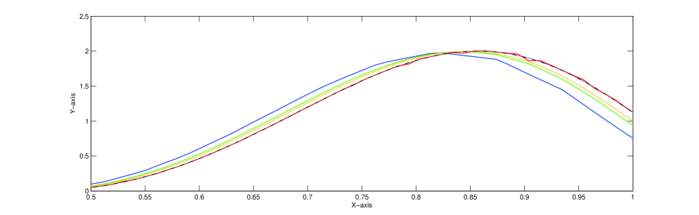
Refer to caption
Figure 1: This figure shows the approximation of f(x)=(1cos(4ex)),x[0.5,1]f(x)=(1-\cos(4e^{x})),\ x\in[0.5,1] (Black) by (I15B¯2f)(x)(I_{15}^{\bar{B}_{2}}f)(x) (Blue), (I2×15B¯2f)(x)(I_{2\times 15}^{\bar{B}_{2}}f)(x) (Green), (I3×15B¯2f)(x)(I_{3\times 15}^{\bar{B}_{2}}f)(x) (Yellow) and (I15,3B¯2f)(x)(I_{15,3}^{\bar{B}_{2}}f)(x) (Red) respectively.
Table 1

Error estimation (upto 44 decimal points) in the approximation of f(x)f(x) by (Iw,3χf)(x)(I_{w,3}^{\chi}f)(x) and (Iiwχf)(x)(I_{iw}^{\chi}f)(x) for i=1,2,3i=1,2,3 and w=15.w=15.

xx |f(x)I15B¯2f(x)||f(x)-I_{15}^{\bar{B}_{2}}f(x)| |f(x)I2×15B¯2f(x)||f(x)-I_{2\times 15}^{\bar{B}_{2}}f(x)| |f(x)I3×15B¯2f(x)||f(x)-I_{3\times 15}^{\bar{B}_{2}}f(x)| |f(x)I15,3B¯2f(x)||f(x)-I_{15,3}^{\bar{B}_{2}}f(x)|
0.600.60 0.14220.1422 0.06640.0664 0.04240.0424 0.00390.0039
0.750.75 0.14740.1474 0.08070.0807 0.05610.0561 0.00330.0033
0.800.80 0.06130.0613 0.04620.0462 0.03590.0359 0.00700.0070
0.900.90 0.21820.2182 0.08000.0800 0.04990.0499 0.01360.0136
0.950.95 0.32300.3230 0.15200.1520 0.09630.0963 0.01290.0129

Now let us consider 4th4^{th} order Mellin B-spline function B¯4(x).\bar{B}_{4}(x). From the Mellin’s Poisson summation formula, we obtain m0(B¯4)=1,m1(B¯4)=0,m2(B¯4)=13,m3(B¯4)=0.m_{0}(\bar{B}_{4})=1,\ m_{1}(\bar{B}_{4})=0,\ m_{2}(\bar{B}_{4})=\frac{1}{3},\ m_{3}(\bar{B}_{4})=0. Now for fC(2)(+),f\in C^{(2)}(\mathbb{R}^{+}), we have the asymptotic formula as

limw+w[(IwB¯4f)(x)f(x)]=(θf)(x)2.\lim_{w\rightarrow+\infty}w[(I_{w}^{\bar{B}_{4}}f)(x)-f(x)]=\frac{(\theta f)(x)}{2}.

But in view of (4.3) and Corollary 2, we obtain the following asymptotic formula

limw+w2[Iw,2B¯4f)(x)f(x)]=(θ2f)(x)6.\lim_{w\rightarrow+\infty}w^{2}[I_{w,2}^{\bar{B}_{4}}f)(x)-f(x)]=\frac{-(\theta^{2}f)(x)}{6}.

This clearly shows that the combination (4.3) provides the order of convergence atleast 2 in asymptotic formula for fC(2)(+).f\in C^{(2)}(\mathbb{R}^{+}). Subsequently, let p=3p=3 and fC(r)(+),r3.f\in C^{(r)}(\mathbb{R}^{+}),\ r\geq 3. In view of Theorem 1, we have the following asymptotic formula

limw+w[(IwB¯4f)(x)f(x)]=(θf)(x)2.\lim_{w\rightarrow+\infty}w[(I_{w}^{\bar{B}_{4}}f)(x)-f(x)]=\frac{(\theta f)(x)}{2}.

But the combination (4.4) provides the following asymptotic formula

limw+w3[(IwB¯4f)(x)f(x)]=(θ3f)(x)48\lim_{w\rightarrow+\infty}w^{3}[(I_{w}^{\bar{B}_{4}}f)(x)-f(x)]=\frac{(\theta^{3}f)(x)}{48}

which ensures the rate of convergence atleast 3 for
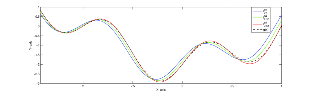
 fC(3)(+).f\in C^{(3)}(\mathbb{R}^{+}).

Refer to caption
Figure 2: This figure shows the approximation of g(x)=sin(2πx)+2sin(πx2),x[π2,4]g(x)=\sin(2\pi x)+2\sin\left(\frac{\pi x}{2}\right),\ x\in\left[\frac{\pi}{2},4\right] (Black) by (I30B¯4g)(x)(I_{30}^{\bar{B}_{4}}g)(x) (Blue), (I2×30B¯4g)(x)(I_{2\times 30}^{\bar{B}_{4}}g)(x) (Green) and (I30,2B¯4g)(x)(I_{30,2}^{\bar{B}_{4}}g)(x) (Red) respectively.
Table 2

Error estimation (upto 44 decimal points) in the approximation of g(x)g(x) by (Iw,2B¯4f)(x)(I_{w,2}^{\bar{B}_{4}}f)(x) and (IiwB¯4f)(x)(I_{iw}^{\bar{B}_{4}}f)(x) for i=1,2i=1,2 and w=30.w=30.

xx |g(x)I30B¯4g(x)||g(x)-I_{30}^{\bar{B}_{4}}g(x)| |g(x)I2×30B¯4g(x)||g(x)-I_{2\times 30}^{\bar{B}_{4}}g(x)| |g(x)I30,2B¯4g(x)||g(x)-I_{30,2}^{\bar{B}_{4}}g(x)|
1.91.9 0.08800.0880 0.03850.0385 0.01100.0110
2.62.6 0.22170.2217 0.13250.1325 0.04340.0434
3.13.1 0.20370.2037 0.12580.1258 0.04790.0479
3.83.8 0.49480.4948 0.20710.2071 0.08060.0806

Now we consider the linear combination of the Mellin’s B-spline functions of order nn as follows:

χ(x)\displaystyle\chi(x) :=\displaystyle:= c1[ταB¯n(x)]+c2[τβB¯n(x)]\displaystyle c_{1}[\tau_{\alpha}\bar{B}_{n}(x)]+c_{2}[\tau_{\beta}\bar{B}_{n}(x)]
=\displaystyle= c1[B¯n(αx)]+c2[B¯n(βx)],\displaystyle c_{1}[\bar{B}_{n}(\alpha x)]+c_{2}[\bar{B}_{n}(\beta x)],\hskip 8.5359pt

Here, τh\tau_{h} represents h-translates of the function B¯n(x)\bar{B}_{n}(x) and is defined as (τhf)(x):=f(hx).(\tau_{h}f)(x):=f(hx). The Mellin’s transformation of χ(x)\chi(x) is given by

M^[χ](w)\displaystyle\hat{M}[\chi](w) =\displaystyle= c1M^[B¯n(αx)]+c2M^[B¯n(βx)]\displaystyle c_{1}\hat{M}[\bar{B}_{n}(\alpha x)]+c_{2}\hat{M}[\bar{B}_{n}(\beta x)] (5.6)
=\displaystyle= c1αwM^[B¯n](w)+c2βwM^[B¯n](w),\displaystyle c_{1}\ \alpha^{-w}\hat{M}[\bar{B}_{n}](w)+c_{2}\ \beta^{-w}\hat{M}[\bar{B}_{n}](w),

which gives

M^[χ](2kπi)=c1α2kπiM^[B¯](2kπi)+c2β2kπiM^[B¯](2kπi).\hat{M}[\chi](2k\pi i)=c_{1}\alpha^{-2k\pi i}\hat{M}[\bar{B}](2k\pi i)+c_{2}\ \beta^{-2k\pi i}\hat{M}[\bar{B}](2k\pi i).

Again from (5.6), we write

M^[χ](w)=c1(αw(M^[B¯](w)αwlogα))+c2(αw(M^[B¯](w)βwlogβ)).\hat{M}^{{}^{\prime}}[\chi](w)=c_{1}(\alpha^{-w}(\hat{M}^{{}^{\prime}}[\bar{B}](w)-\alpha^{-w}\log\alpha))+c_{2}(\alpha^{-w}(\hat{M}^{{}^{\prime}}[\bar{B}](w)-\beta^{-w}\log\beta)).

In view of Lemma 1 in [34], we obtain

c1+c2=1,c1logα+c2logβ=0.c_{1}+c_{2}=1\ ,\ \ c_{1}\log\alpha+c_{2}\log\beta=0.

On solving for c1andc2,c_{1}\ \ \mbox{and}\ \ c_{2}, we get

c1=logβ(logβlogα),c2=logα(logβlogα).c_{1}=\frac{\log\beta}{(log\beta-\log\alpha)},\ \ c_{2}=\frac{-\log\alpha}{(\log\beta-log\alpha)}.

In particular for α=e\alpha=e and β=e2,\beta=e^{2}, we obtain the following linear combination of the Mellin’s B-spline of order 4

χ(x)=2B¯4(ex)B¯4(e2x),x+.\chi(x)=2\bar{B}_{4}(ex)-\bar{B}_{4}(e^{2}x)\ ,\ \ x\in\mathbb{R}^{+}.

Indeed, it satisfies all the assumptions of the kernel function. Again by using the Mellin’s Poisson summation formula, we obtain

m0(χ)=1,m1(χ)=0,m2(χ)=53.m_{0}(\chi)=1,\ m_{1}(\chi)=0,\ m_{2}(\chi)=\frac{-5}{3}.

Now for fC(2)(+)f\in C^{(2)}(\mathbb{R}^{+}) and p=2,p=2, we have the following asymptotic formulae for the operators (Iwχf)(I_{w}^{\chi}f) and (Iw,2χf),(I_{w,2}^{\chi}f),

limw+w[(Iwχf)(x)f(x)]=(θf)(x)2\lim_{w\rightarrow+\infty}w[(I_{w}^{\chi}f)(x)-f(x)]=\frac{(\theta f)(x)}{2}

and

limw+w2[(Iw,2χf)(x)f(x)]=13(θ2f)(x).\lim_{w\rightarrow+\infty}w^{2}[(I_{w,2}^{\chi}f)(x)-f(x)]=\frac{1}{3}(\theta^{2}f)(x).

Evidently, the combination (4.3) shows the convergence of order atleast 2 for fC(2)(+).f\in C^{(2)}(\mathbb{R}^{+}).

References

  • [1] Angamuthu, S.K., Ponnaian, D.; Approximation by generalized bivariate Kantorovich sampling type series. J Anal. 27, 429-449 (2019).
  • [2] Agrawal, P.N., Prasad, G; Degree of approximation to integrable functions by Kantorovich polynomials, Boll. Un. Mat. Ital. A (6) 4 , 323-326 (1985).
  • [3] Balsamo, S., Mantellini, I.; On linear combinations of general exponential sampling series, Results Math. 74 (180) (2019).
  • [4] Bardaro, C., Butzer, P.L., Stens, R.L., Vinti, G.; Approximation of the Whittaker Sampling Series in terms of an Average Modulus of Smoothness covering Discontinuous Signals. J. Math. Anal. Appl. 316, 269-306(2006).
  • [5] Bardaro, C., Vinti, G., Butzer, P.L., Stens, R.; Kantorovich-type generalized sampling series in the setting of Orlicz spaces. Sampl. Theory Signal Image Process. 6, 29-52 (2007).
  • [6] Bardaro, C., Mantellini, I.; A quantitative Voronovskaja formula for generalized sampling operators, East J. Approx. 15 (4) , 459-471(2009).
  • [7] Bardaro, C., Mantellini, I.; Voronovskaya formulae for Kantorovich type generalized sampling series. Int. J. Pure Appl. Math. 62 , 247-262 (2010).
  • [8] Bardaro, C., Butzer, P.L., Stens, R., Vinti, G.; Prediction by samples from the past with error estimates covering discontinuous signals, IEEE Transactions on Information Theory. 56(1), 614-633(2010).
  • [9] Bardaro, C., Mantellini, I.; On convergence properties for a class of Kantorovich discrete operators. Numer. Funct. Anal. Optim. 33 , 374-396 (2012).
  • [10] Bardaro, C., Mantellini, I.; Asymptotic formulae for linear combinations of generalized sampling type operators. Z. Anal. Anwend. 32(3), 279-298 (2013).
  • [11] Bardaro, C., Mantellini, I; On Linear Combinations of Multivariate Generalized Sampling Type Series. Mediterr. J. Math. 10, 1833-1852 (2013).
  • [12] Bardaro, C., Butzer, P.L., Mantellini, I.; The exponential sampling theorem of signal analysis and the reproducing kernel formula in the Mellin transform setting. Sampl. Theory Signal Image Process. 13, 35-66 (2014).
  • [13] Bardaro, C., Mantellini, I.; On Mellin convolution operators: a direct approach to the asymptotic formulae. Integral Transforms Spec. Funct. 25, 182-195 (2014).
  • [14] Bardaro, C., Butzer, P.L., Mantellini, I.; The Mellin-Parseval formula and its interconnections with the exponential sampling theorem of optical physics. Integral Transforms Spec. Funct. 27, 17-29(2016).
  • [15] Bardaro, C., Butzer, P.L., Mantellini, I., Schmeisser, G.; On the Paley-Wiener theorem in the Mellin transform setting. J. Approx. Theory. 207, 60-75(2016).
  • [16] Bardaro, C., Faina, L., Mantellini, I.; A generalization of the exponential sampling series and its approximation properties. Math. Slovaca 67 , 1481-1496 (2017).
  • [17] Bardaro, C., Mantellini, I., Sch meisser, G.; Exponential sampling series: convergence in Mellin-Lebesgue spaces. Results Math. 74 (2019), no. 3, Art. 119, 20 pp.
  • [18] Bardaro, C., Bevignani, G., Mantellini, I., Seracini, M.; Bivariate Generalized Exponential Sampling Series and Applications to Seismic Waves, Constructive Mathematical Analysis, 2 , 153-167(2019).
  • [19] Bertero, M., Pike, E.R.; Exponential-sampling method for Laplace and other dilationally invariant transforms. II. Examples in photon correlation spectroscopy and Fraunhofer diffraction. Inverse Problems 7, 21-41(1991).
  • [20] Butzer, P.L., Linear Combinations of Bernstein Polynomials. Canad. J. Math. 5, 559-567(1953).
  • [21] Casasent, D.; Optical data processing, Springer, Berlin, 241-282 (1978).
  • [22] Butzer, P. L., Ries, S., Stens, R. L.; Approximation of continuous and discontinuous functions by generalized sampling series, J. Approx. Theory. 50, 25-39(1987).
  • [23] Butzer, P. L., Stens, R. L.; Prediction of non-bandlimited signals from past samples in terms of splines of low degree, Math. Nachr. 132 , 115-130(1987).
  • [24] Butzer, P. L., Stens, R. L.; Sampling theory for not necessarily band-limited functions: an historical overview, SIAM Review. 34, 40-53(1992).
  • [25] Butzer, P.L., Stens, R.L.; Linear prediction by samples from the past, In: Advanced Topics in Shannon Sampling and Interpolation Theory ,Springer Texts Electrical Eng., Springer, New York, 157-183(1993).
  • [26] Butzer, P.L., Jansche, S.; A direct approach to the Mellin transform. J. Fourier Anal. Appl. 3, 325-376(1997).
  • [27] Butzer, P.L., Jansche, S.; The exponential sampling theorem of signal analysis, Dedicated to Prof. C. Vinti (Italian) (Perugia, 1996), Atti. Sem. Mat. Fis. Univ. Modena, Suppl. 46 , 99-122(1998).
  • [28] Butzer, P.L., Stens, R.L.; A self contained approach to Mellin transform analysis for square integrable functions;applications. Integral Transform. Spec. Funct. 8 ,175-198(1999).
  • [29] Cluni, F., Costarelli, D., Minotti, A.M., Vinti, G.; Applications of sampling Kantorovich operators to thermographic images for seismic engineering. J. Comput. Anal. Appl. 19 , 602-617(2015).
  • [30] Costarelli, D., Minotti, A.M., Vinti, G.; Approximation of discontinuous signals by sampling Kantorovich series. J. Math. Anal. Appl. 450, 1083-1103(2017).
  • [31] Costarelli, D., Vinti, G.; Inverse results of approximation and the saturation order for the sampling Kantorovich series. J. Approx. Theory 242, 64-82(2019).
  • [32] Gori, F.; Sampling in optics. Advanced topics in Shannon sampling and interpolation theory, 37-83, Springer Texts Electrical Engrg., Springer, New York, 1993.
  • [33] Gupta, V., Tachev, G., Acu, A.M., Modified Kantorovich operators with better approximation properties. Numer. Algorithms 81, 125-149 (2019).
  • [34] Kumar, A.S., Shivam, B.; Direct and inverse results for Kantorovich type exponential sampling series. arXiv:submit/2992999, (2020)
  • [35] Kumar, A.S., Shivam, B.; Inverse approximation and GBS of bivariate Kantorovich type sampling series. RACSAM 114, 82 (2020).
  • [36] Kumar, A. S., Pourgholamhossein, M., Tabatabaie, S. M.; Generalized Kantorovich sampling type series on hypergroups. Novi Sad J. Math. 48 ,117-127(2018).
  • [37] May, C. P.; Saturation and inverse theorems for combinations of a class of exponential-type operators. Canadian J. Math. 28 , 1224-1250(1976).
  • [38] Mamedov, R.G.; The Mellin transform and approximation theory , ”Elm”, Baku, 1991, 273 pp.
  • [39] Orlova, O., Tamberg, G.; On approximation properties of generalized Kantorovich-type sampling operators, J. Approx. Theory, 201 , 73-86(2016).
  • [40] Ostrowsky, N., Sornette, D., Parke, P., Pike, E.R.; Exponential sampling method for light scattering polydispersity analysis, Opt. Acta. 28 , 1059-1070(1994).
  • [41] Ries, S., Stens, R. L.; Approximation by generalized sampling series, In Constructive Theory of Functions, Proc. Conf. Varna, 1984, edited by Bl. Sendov et al., Publ. House Bulgarian Acad. Sci, Sofia, 746-756(1984).
  • [42] Vinti, G., Luca, Z., Approximation results for a general class of Kantorovich type operators. Adv. Nonlinear Stud. 14, 991-1011(2014).