Omni-resonant imaging across the visible

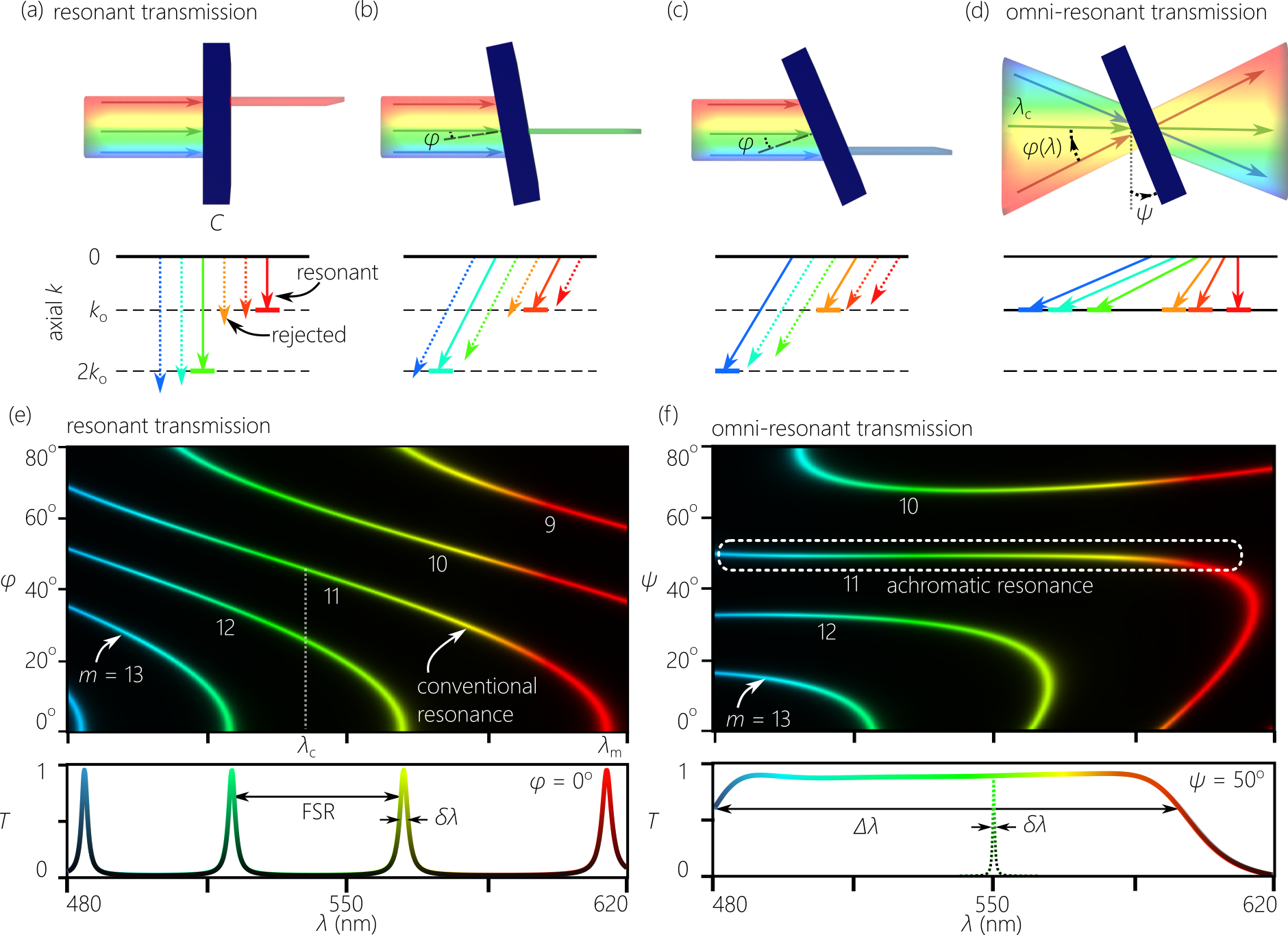
To set the stage for the realization of omni-resonant imaging, we compare in Fig. 1 three basic configurations. In conventional ‘white-light imaging’ [Fig. 1(a)], light from a broadband source $\mathcal{S}$ scatters from an object $\mathcal{O}$, which is located at a distance $d_{1}$ from a lens L (focal length $f$), and an image is formed at distance $d_{2}$ at a detector $\mathcal{D}$, where $\tfrac{1}{d_{1}}+\tfrac{1}{d_{2}}\!=\!\tfrac{1}{f}$. The ‘resonant imaging’ configuration in Fig. 1(b), in which an FP cavity is placed in the conventional imaging system, can enhance optical effects of relevance to imaging, but most of the spectrum from $\mathcal{S}$ is rejected and image formation makes use of light only on resonance. The recently reported degenerate-cavity configuration in Yevgeny et al. (2022) enables coupling a spatially multimoded field into an FP cavity (by placing an imaging system inside the cavity Arnaud (1969); Tradonsky et al. (2019)), but once again only on resonance. We aim here at image formation through the FP cavity over a broad, continuous spectrum (ideally, across the entire visible spectrum), which we refer to as ‘omni-resonant imaging’ [Fig. 1(c)] by pre-conditioning the incident field. Subsequently, the field emerging from the FP cavity is post-conditioned to produce a total point-spread function in the form of an impulse (point-by-point imaging or field relay) from the entrance of the omni-resonant system to its exit. Image formation then relies on external lenses, without the cavity reducing the useful source spectrum.

To elucidate the concept of omni-resonance, we first note some salient features of conventional FP resonances at oblique incidence. Consider a symmetric cavity of finesse $\mathcal{F}$ formed of two mirrors separated by a transparent layer of thickness $d$ and refractive index $n$. When collimated broadband light impinges on the cavity at an angle $\varphi$ with respect to its normal, resonances occur when $\chi(\lambda,\varphi)\!=\!2\pi m$. The wavelength associated with the $m^{\mathrm{th}}$ resonance varies widely with $\varphi$, from $\lambda_{m}\!=\!\tfrac{2nd}{m}$ at normal incidence [Fig. 2(a)] to a blue-shifted wavelength $\lambda_{\mathrm{min}}\!=\!\lambda_{m}(1-\sigma_{n})$ [Fig. 2(b,c)] at glancing incidence ($\varphi\!\rightarrow\!90^{\circ}$); where we have defined for convenience the parameter $\sigma_{n}\!=\!1-\sqrt{1-\tfrac{1}{n^{2}}}$. The maximum bandwidth associated in principle with the $m^{\mathrm{th}}$-resonance is therefore $\Delta\lambda_{m}\!=\!\lambda_{m}-\lambda_{\mathrm{min}}\!=\!\sigma_{n}\lambda_{m}$, which is significantly larger than the resonant linewidth $\delta\lambda$: $\tfrac{\Delta\lambda_{m}}{\delta\lambda}\!=\!(m+1)\sigma_{n}\mathcal{F}\!\gg\!1$; and can even be larger than the FSR: $\tfrac{\Delta\lambda_{m}}{\mathrm{{FSR}}}\!=\!(m+1)\sigma_{n}$. Conventional FP resonances are therefore intrinsically characterized by AD Torres et al. (2010); that is, for the $m^{\mathrm{th}}$ resonance, each wavelength $\lambda$ within $\Delta\lambda_{m}$ is associated with a particular incident angle $\varphi(\lambda)$ to satisfy the resonance condition. We plot in Fig. 2(e) the spectral transmission $T(\lambda,\varphi)$ for an FP cavity with $n\!=\!1.49$, $d\!=\!2.5$ $\mu$m, and $\mathcal{F}\!=\!30$. The $m=11$ resonance at normal incidence occurs at $\lambda_{11}\!=\!612$ nm, the FSR is $\approx\!45$ nm, and the full bandwidth associated in principle with this resonance is $\Delta\lambda_{11}\!\approx\!158$ nm (Methods).

These characteristics of conventional FP resonances suggest a strategy for broadening the resonant spectral response associated with a fixed-order resonance and without impacting the cavity finesse. The AD profile for an FP resonance is in general nonlinear [Fig. 2(e)], especially in the vicinity of $\lambda_{m}$ and $\lambda_{\mathrm{min}}$. However, the AD profile is approximately linear over a broad span between $\lambda_{m}$ and $\lambda_{\mathrm{min}}$. The condition $\tfrac{d^{2}\varphi}{d\lambda^{2}}\!=\!0$ is satisfied at a wavelength $\lambda_{\mathrm{c}}\!=\!\sqrt{\lambda_{m}\lambda_{\mathrm{min}}}$, which corresponds to an incident angle $\sin\{\varphi(\lambda_{\mathrm{c}})\}\!=\!n\sqrt{\sigma_{n}}$. The AD remains approximately linear in the vicinity of $\lambda_{\mathrm{c}}$, with a first-order AD coefficient $\beta_{m}\!=\!\frac{d\varphi}{d\lambda}\big{|}_{\lambda_{\mathrm{c}}}\!=\!-\frac{1}{\Delta\lambda_{m}}$. Therefore, by externally introducing linear AD into the incident optical field to match the FP-resonance [Fig. 2(d)], a broad spectrum can resonate continuously with the cavity while remaining associated with the $m^{\mathrm{th}}$ resonance. This is accomplished by directing each wavelength $\lambda$ to the FP cavity at an angle $\varphi(\lambda)\!=\!\psi+\beta_{m}(\lambda-\lambda_{\mathrm{c}})$, such that the wavelength $\lambda_{\mathrm{c}}$ is incident at an angle $\psi$ onto the FP cavity, and the other wavelengths are angularly distributed linearly around $\psi$. When the cavity is tilted such that $\psi\!=\!\varphi(\lambda_{\mathrm{c}})$, which we call the omni-resonant condition, a broad spectrum centered on $\lambda_{\mathrm{c}}$ resonates continuously with the FP cavity and remains in its entirety associated with the same resonant order $m$.

We plot in Fig. 2(f) the spectral transmission $T(\lambda,\psi)$ through the same FP cavity employed in Fig. 2(e) after introducing an AD profile $\varphi(\lambda)\!=\!\psi+\beta_{11}(\lambda-\lambda_{\mathrm{c}})$, where $\beta_{11}\!\approx\!-0.36$ ^∘/nm and $\lambda_{\mathrm{c}}\!\approx\!530$ nm (Methods), resulting in an achromatic resonance at $\psi\!=\!\varphi(\lambda_{\mathrm{c}})\!\approx\!50^{\circ}$. Once the cavity is tilted away from this angle, the achromatic resonance disappears. The omni-resonant bandwidth associated with $m\!=\!11$ is $\Delta\lambda\!\approx\!130$ nm [Fig. 2(f)]. While holding the AD coefficient $\beta_{11}$ fixed, other achromatic resonances occur while varying $\psi$ that are associated with different $m$; e.g., $m\!=\!12$ at $\psi\!\approx\!35^{\circ}$ [Fig. 2(f)]. However, the bandwidths of these other achromatic resonances are sub-optimal. Finally, we note that we included in the calculation in Fig. 2(f) an additional nonlinear component to $\varphi(\lambda)$, which arises in our experimental setup in Fig. 3(a) and further improves the omni-resonant bandwidth over that resulting from strictly linear AD (Methods).

The FP cavity we make use of here consists of a pair of dielectric Bragg mirrors sandwiching a $\approx 2.2$-$\upmu$m-thick SiO₂ layer. Each mirror is formed of 8 alternating bilayers of TiO₂ and SiO₂ (refractive indices of $\approx\!1.49$ and $2.28$, respectively, at $\lambda\!\sim\!540$ nm). The resulting Bragg reflectance is $\approx\!98\%$ over a 180-nm-bandwidth ($\sim\!500\!-\!680$ nm), a finesse $\mathcal{F}\!\approx\!85$, resonance linewidth $\approx 0.5$ nm, free spectral range $\approx 45$ nm, and normal-incidence resonant wavelengths $\lambda_{m}\approx 522$, 565, and 610 nm for $m\!=\!13$, 12, and 11, respectively. The value of AD required to excite an achromatic resonance associated with $m\!=\!11$ ($\beta_{11}\!=\!-0.36$ ^∘/nm) is significantly larger than can be achieved simply by a diffraction grating Saleh and Teich (2007) or a metasurface Arbabi et al. (2017) in the visible. Instead, we realize the requisite AD profile using the setups shown in Fig. 3(a,d), which have the same overall structure. First, a diffraction grating introduces linear AD of value $\beta\!<\!\beta_{11}$, followed by an achromatic biconvex lens L₁ that collimates the spectrum at a plane denoted the ‘input plane’. The bandwidth intercepted by the aperture of L₁ is determined by $\beta$, and the wavelength $\lambda_{\mathrm{c}}$ coincides with the symmetry axis of the system. Following L₁, lenses are used to increase the value of $\beta$ to reach $\beta_{11}$, and the field then impinges on the FP cavity, which is tilted an angle $\psi$ with respect to the wavelength $\lambda_{\mathrm{c}}$. The optical system following the FP cavity mirrors that preceding it in order to reconstitute the spectrum into a collimated beam. An ‘output plane’ after the FP cavity, where the white-light spectrum is spatially resolved, mirrors the location of the input plane preceding it. A measurement at this plane unveils whether conventional FP resonances (discrete, sparse spectrum) or an achromatic resonance (continuous, broadband spectrum) have been excited. Between the two gratings, the wave front is spectrally resolved in space, which necessitates careful design to minimize chromatic and spherical aberrations.

In the first setup [Fig. 3(a)], the grating $G_{1}^{\prime}$ produces $\beta\approx-0.05$ ^∘/nm and the bandwidth intercepted by L₁ is $\approx 190$ nm. The linear AD coefficient is subsequently increased by $7\times$ using an afocal magnification system comprising L₁ and a plano-convex aspheric condenser lens L${}_{2}^{\prime}$ (Methods). We plot in Fig. 3(b) the calculated AD profile $\varphi(\lambda)$ produced by this setup, and compare it to the spectral trajectory of the conventional FP resonance $m\!=\!11$. Note that the predicted AD profile matches the finesse-limited FP resonance over a broad bandwidth. The AD produced after L${}_{2}^{\prime}$ is not purely linear, because the local curvature along the lens surface varies with height. As shown in Fig. 3(b), inset, L${}_{2}^{\prime}$ has a prescribed lens ‘sag’, a height-dependent lens thickness $z(h)$, from which we calculate the local lens curvature Geary (2002) ($h$ is the height from the optical axis). For a collimated field incident on L${}_{2}^{\prime}$ (prepared by L₁) we calculate the angle $\varphi(h)$ with the $z$-axis that a ray incident on the curved surface of L${}_{2}^{\prime}$ at height $h$ emerges from its planar surface. Because the ray at height $h$ is associated with a particular wavelength $\lambda$, we readily obtain the AD profile $\varphi(\lambda)$ (Methods). For wavelengths close to $\lambda_{\mathrm{c}}$ in the vicinity of the optical axis, $\varphi(\lambda)$ is approximately linear in $\lambda$. However, the extreme ends of the incident spectrum that reach the edges of L${}_{2}^{\prime}$ have an AD profile with a significant nonlinear contribution. The particular sag profile of L${}_{2}^{\prime}$ produces a nonlinear AD profile $\varphi(\lambda)$ away from $\lambda_{\mathrm{c}}$ that matches the spectral trajectory of the FP resonance $m\!=\!11$, thus extending the omni-resonant bandwidth beyond that afforded by linear AD.

To verify omni-resonant transmission, we direct white-light to G${}_{1}^{\prime}$ in absence of an object, and plot in Fig. 3(c) three spatially resolved spectra recorded by a color CCD camera (Sony $\alpha 6000$): (1) the spectrum at the input plane, which corresponds to an intercepted bandwidth $\approx 190$ nm from the source as determined by G${}_{1}^{\prime}$ and the aperture of L₁; (2) the conventional resonant spectrum transmitted through the FP cavity at normal incidence in absence of AD(corresponding to resonances $m\!=\!13$, 12, and 11 at wavelengths $\approx\!522$, 565, and 610 nm, respectively); and (3) the spectrum at the output plane transmitted through the FP cavity. The conventional resonant spectrum is obtained by directing the collimated white-light source normally to the FP cavity, and then spatially resolving the transmitted spectrum via G${}_{1}^{\prime}$ and L₁. We observe in the output spectrum an achromatic resonance of bandwidth $\Delta\lambda\!\approx\!130$ nm associated with $m\!=\!11$. Not only does this bandwidth far exceed the resonant linewidth, but it also exceeds twice the FSR. This is the largest resonant linewidth enhancement factor reported to date using any technique.

However, calculations and measurements reveal that this system is associated with significant spherical aberrations associated with the use of the aspheric lens L${}_{2}^{\prime}$, especially at wavelengths far away from the central wavelength of 550 nm; see Fig. 3(b) and Methods. To minimize these aberrations, we employ the setup shown in Fig. 3(d) in which the grating G₁ introduces higher AD of $\beta\!\approx\!-0.09$ ^∘/nm, and we replace the aspheric lens L${}_{2}^{\prime}$ with a pair of achromatic lenses L₂ and L₃ that comprise an afocal imaging telescope. This system increases the AD by $4\times$ and produces AD that is closer to a linear profile; see Fig. 3(e) and Methods. Calculations reveal spherical aberrations of $\sim\!0.2$ wavelengths for an entrance pupil of diameter 20 mm Geary (2002), thus producing an Airy radius of 36 $\upmu$m that contains within it the majority of the incident spectrum [Fig. 3(e), inset]. This latter requirement is critical to achieve high-quality broadband color-imaging. The measured input, resonant, and omni-resonant spectra for the setup in Fig. 3(d) are plotted in Fig. 3(f). The input spectrum intercepted by L₁ is reduced to $\approx 100$ nm ($\sim 520-620$ nm) because of the larger AD from G₁, and an omni-resonant bandwidth $\approx 100$ nm is observed at the output plane.

The full picture of the resonant and omni-resonant spectral responses are shown in Fig. 4. We first plot in Fig. 4(a,b) the measured conventional resonant transmission spectra through the FP cavity obtained using collimated white light while varying the incident angle $\varphi$, which reveals the spectral trajectories of the conventional FP resonances $m\!=\!10-13$ (Supplementary Movie 1). We then plot in Fig. 4(c,d) the measured transmission through the same cavity after introducing AD using the setup in Fig. 3(a) while varying $\psi$ (Supplementary Movie 2). The optimal achromatic resonance associated with $m\!=\!11$ appears at $\psi\approx 50^{\circ}$ extending over the green and red portions of the visible spectrum, while a sub-optimal achromatic resonance associated with $m\!=\!12$ appears at $\psi\approx 35^{\circ}$ and dominated by the blue portion of the visible spectrum. Similar results are obtained using the setup in Fig. 3(d) except for smaller bandwidths achieved for the achromatic resonances.

We have confirmed above the significant resonant spectral broadening afforded by the omni-resonant configuration. Calculations for the setup in Fig. 3(d) predict low imaging aberrations despite this spectral broadening, which indicates that broadband imaging can be carried out through such a system. We next verify omni-resonant imaging using objects in the form of transmissive color transparencies. The collimated white-light source is transmitted through the object, and the spatially structured field impinges on the omni-resonant FP cavity system [Fig. 3(d)], and a biconvex lens (focal length $f\!=\!100$ mm) forms an image that is captured with a color camera (Sony $\alpha 6000$). Because this omni-resonant configuration corresponds to a point-to-point relay system, the axial extent from G₁ (the entrance plane) to G₂ (the exit plane) does not contribute to image formation [Fig. 1(c)]. Excluding the omni-resonant system, the distance from the object plane to the lens is $d_{1}\!=\!300$ mm, and from the lens to the image plane $d_{2}\!=\!150$ mm.

We make use of three objects to test the omni-resonant imaging system, each displaying a Pegasus of dimensions $15\!\times\!15$ mm² colored blue, green, and red. The images captured by the color camera are displayed in Fig. 5(a-c). In each case, we show a reference image of the object and the corresponding omni-resonant image. The reference image is acquired by placing the object after the omni-resonant system, which simply delivers a collimated white-light field whose spectrum is filtered to a bandwidth $\Delta\lambda\approx 100$ nm. The omni-resonant image, on the other hand, is acquired by placing the object before the omni-resonant system, in which case the broadband optical field incident on G₁ is spatially structured. Nevertheless, the reference and omni-resonant images formed are identical. This indicates that the omni-resonant system does not hinder the image-formation process. Next we make use of objects in the form of a multi-colored Pegasus as shown in Fig. 5(d,e), and once again we find excellent agreement between the reference and omni-resonant images. Finally, we make use of a black-and-white Pegasus as shown in Fig. 5(f). The image in this last case appears yellow rather than white because the blue part of the visible spectrum is not included in the omni-resonant bandwidth [Fig. 3(f)]. In the images displayed in Fig. 5(b-f), we make use of the achromatic resonance associated with $m\!=\!11$ (at $\psi\!\approx\!50^{\circ}$). This achromatic resonance is truncated at the blue-end of the spectrum, and extends from the green ($\approx 520$ nm) to the red ($\approx 620$ nm). To produce the blue image in Fig. 5(a), we made use of the sub-optimal achromatic resonance associated with $m\!=\!12$, which is excited at $\psi\!\approx\!35^{\circ}$ after adjusting the incident angle on G₁ to $15^{\circ}$ to arrange for the blue portion of the spectrum to impinge on the FP cavity. This partial achromatic resonance extends from the blue ($\sim 485$ nm) to the green ($\sim 530$ nm). Hence, full-color visible omni-resonant imaging has not yet been realized using a single achromatic resonance. We investigate this limit further in the Discussion.

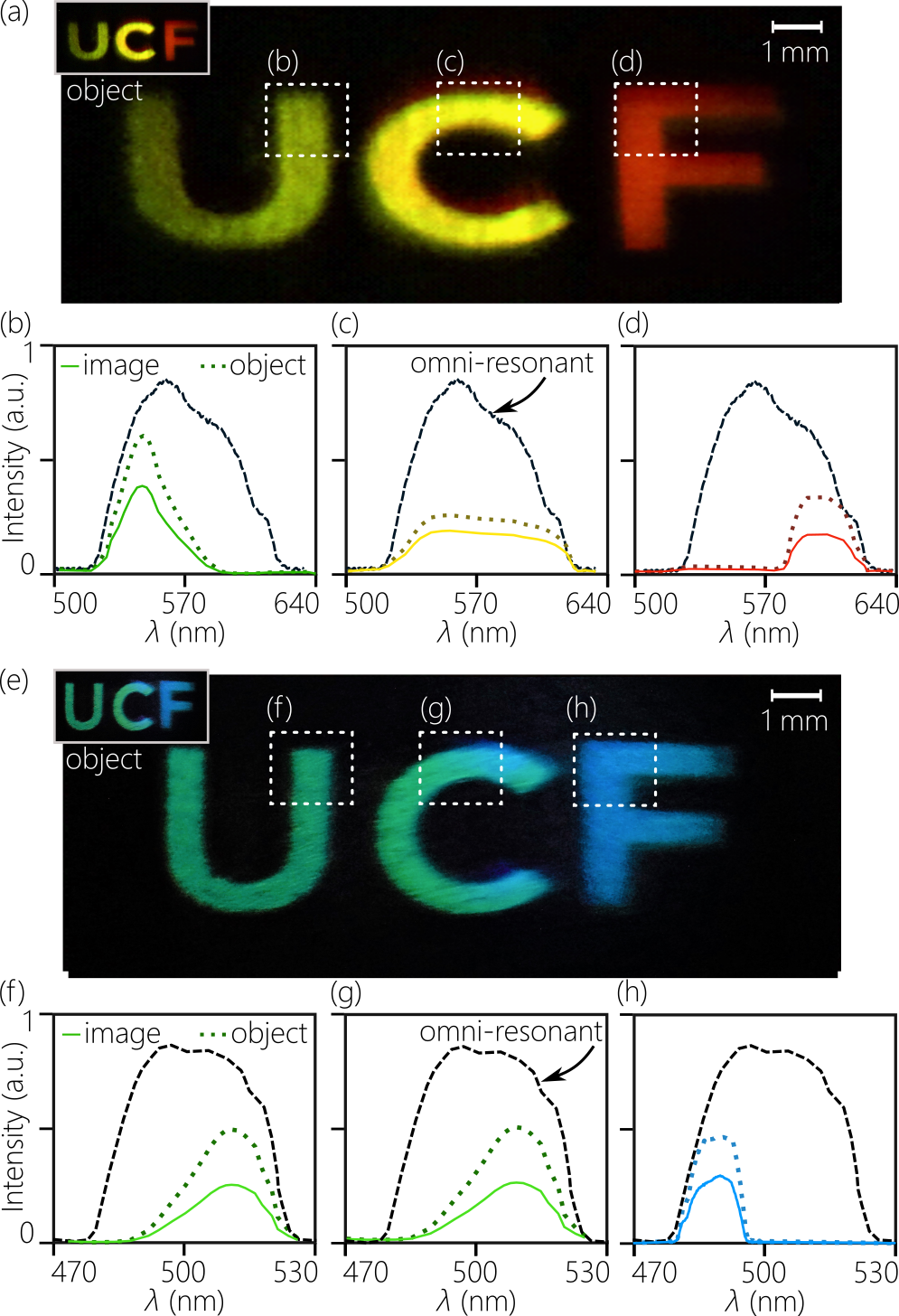
To verify quantitatively that the colors captured in the omni-resonant image correspond to those in the object, we make use of an object displaying different-colored letters ‘UCF’ (with dimensions $10\!\times\!4$ mm²). The omni-resonant image is shown in Fig. 6(a), and the reference image is shown as the inset. We capture with a multimode fiber light from each letter corresponding to the highlighted regions in Fig. 6(a), and then compare the measured spectra in the omni-resonant and reference images to the transmitted spectra through the same portions of the object when illuminated with the collimated 100-nm-bandwidth omni-resonant spectrum [Fig. 6(b-d)]. The object and image spectra are almost identical, thereby confirming the spectral fidelity of the omni-resonant color-imaging system. We repeat these measurements with an object whose colors are predominantly blue [Fig. 6(e)], where we made use of the $m\!=\!12$ partial achromatic resonance described above. The object and image spectra are in excellent agreement [Fig. 6(f-h)].

The omni-resonant images in Fig. 5 and Fig. 6 made use of incoherent white light. We finally combine coherent and incoherent light in the omni-resonant imaging system [Fig. 7]. The coherent light comprises a pair of laser diodes: laser 1 at a wavelength of 532 nm (Thorlabs CPS532) and laser 2 at a wavelength of 632 nm (Newport N-LHP-111). The white light and the laser beams are combined on a beam splitter. The spectrum of the combined source is measured in absence of the object at the input plane (prior to the FP cavity) and the output plane (after the FP cavity) identified in Fig. 3(d), which are displayed in Fig. 7(a) and Fig. 7(b), respectively. The two spectra are in excellent agreement, and we can clearly discern the broadband incoherent white-light spectrum and the spectrally localized coherent lasers. Next, we insert the black-and-white Pegasus object from Fig. 5(f) into the combined-beam path, and capture the color image as the two laser beams are scanned independently but simultaneously across the plane of the object by displacing the laser beams in the transverse plane. A Supplementary Movie captures in real time the omni-resonant color image produced by the combined source, and Fig. 7(c-e) shows selected still images of the Pegasus object. The extended white-light field-of-view is stationary and illuminates the full object, whereas the green and red laser beams are spatially localized and are scanned independently across the object plane with the captured image tracking their movement in real time.

The spectral transmission of a collimated optical field from free space at a wavelength $\lambda$ incident on a symmetric FP cavity at an angle $\varphi$ with respect to the cavity normal is:

$$T(\lambda,\varphi)=\frac{1}{\{1+\left(\frac{2\mathcal{F}}{\pi}\right)^{2}\sin^{2}\frac{\chi}{2}},$$

(1)

where $\mathcal{F}\!=\!\tfrac{\pi\sqrt{R}}{1-R}$ is the cavity finesse, $R$ the cavity mirror reflectivity, the roundtrip cavity phase is:

$$\chi(\lambda,\varphi)=\frac{4\pi d}{\lambda}\sqrt{n^{2}-\sin^{2}\varphi},$$

(2)

$d$ is the cavity length, and $n$ is its refractive index; we have ignored the phases incurred upon reflection from the cavity mirrors. Resonance occurs at normal incidence at wavelengths $\lambda_{m}\!=\!\tfrac{2nd}{m}$, which correspond to a round-trip phase $\chi(\lambda_{m},0)\!=\!2\pi m$, where integer $m$ is the resonance order [Fig. 2(a)]. At oblique incidence, the resonance condition $\chi(\lambda,\varphi)\!=\!2\pi m$ is maintained for the same-order resonance at a blue-shifted wavelength [Fig. 2(b,c)]:

$$\lambda_{m}(\varphi)=\lambda_{m}\sqrt{1-\tfrac{1}{n^{2}}\sin^{2}\varphi}<\lambda_{m}.$$

(3)

Therefore, wavelengths associated with the $m^{\mathrm{th}}$ resonance range from $\lambda\!=\!\lambda_{m}$ at normal incidence to $\lambda\!=\!\lambda_{\mathrm{min}}\!=\!\lambda_{m}(1-\sigma_{n})$ at glancing angle ($\varphi\!\rightarrow\!90^{\circ}$), where we define for convenience the parameter

$$\sigma_{n}=1-\sqrt{1-\tfrac{1}{n^{2}}},$$

(4)

which depends solely on the cavity refractive index.

The first- and second-order derivatives of $\varphi(\lambda)$ for the $m^{\mathrm{th}}$-resonance are:

	$\displaystyle\frac{d\varphi}{d\lambda}$	$\displaystyle=$	$\displaystyle-\frac{\lambda}{\sqrt{\lambda_{m}^{2}-\lambda^{2}}\sqrt{\lambda^{2}-\lambda_{\mathrm{min}}^{2}}},$		(5)
	$\displaystyle\frac{d^{2}\varphi}{d\lambda^{2}}$	$\displaystyle=$	$\displaystyle\frac{\lambda_{m}^{2}\lambda_{\mathrm{min}}^{2}-\lambda^{4}}{(\lambda_{m}^{2}-\lambda^{2})^{3/2}(\lambda^{2}-\lambda_{\mathrm{min}}^{2})^{3/2}}.$		(6)

Both expressions are valid in the spectral range $\lambda_{\mathrm{min}}\!<\!\lambda\!<\!\lambda_{m}$. Setting $\tfrac{d^{2}\varphi}{d\lambda^{2}}\!=\!0$ in Eq. 6 yields the wavelength:

$$\lambda_{\mathrm{c}}=\sqrt{\lambda_{m}\lambda_{\mathrm{min}}},$$

(7)

which is the geometric mean of the two extreme wavelengths associated with the $m^{\mathrm{th}}$-resonance. Substituting $\lambda\!=\!\lambda_{\mathrm{c}}$ into Eq. 5, we obtain the linear AD coefficient:

$$\beta_{m}=\tfrac{d\varphi}{d\lambda}\big{|}_{\lambda_{\mathrm{c}}}=-\frac{1}{\lambda_{m}-\lambda_{m}^{\mathrm{min}}}=-\frac{1}{\Delta\lambda_{m}}=-\frac{1}{\lambda_{m}\sigma_{n}}.$$

(8)

For $m\!=\!11$, the cavity parameters in the main text yield $\Delta\lambda_{m}\!\approx\!158$ nm and $\beta_{11}\!\approx\!-0.36^{\circ}$/nm.

In both setups in Fig. 3(a) and Fig. 3(d), we make use of a collimated white-light source (Thorlabs MCWHL8), and all the lens apertures are 50 mm in diameter. In the first setup [Fig. 3(a)] we use a diffraction grating $G_{1}^{\prime}$ with groove density 830 lines/mm, area $25\!\times\!25$ mm², an incident angle $20^{\circ}$ with respect to the grating normal, and the -1 diffraction order is selected at an angle of $5^{\circ}$. This configuration provides AD of $\beta\approx-0.05^{\circ}$/nm, which is significantly lower in magnitude than the target value $\beta_{11}\approx-0.36^{\circ}$/nm associated with the $m\!=\!11$ resonance. We increase the value of $\beta$ provided by the grating by a factor $7\times$ before incidence on the FP cavity using an afocal magnification system comprising an achromatic biconvex lens (L₁; $f\!=\!300$ mm), followed by a plano-convex aspheric condenser lens (L${}_{2}^{\prime}$; $f\!=\!40$ mm; Thorlabs ACL5040U). The distance between G${}_{1}^{\prime}$ and L₁ is 300 mm, L₁ and L${}_{2}^{\prime}$ are separated by 330 mm, and the distance from L${}_{2}^{\prime}$ to the FP cavity is 25 mm. The system is then mirrored after the FP cavity to recombine the wavelengths. We describe below in more detail the AD spectral profile produced by the aspheric lens L${}_{2}^{\prime}$.

In the setup shown in Fig. 3(d), light impinges on a diffraction grating G₁ (1400 lines/mm, $25\!\times\!25$-mm² area) at an angle $20^{\circ}$ with respect to its normal, and the -1 diffracted order is selected (diffracted angle $-25^{\circ}$). The AD produced by the grating in this configuration is $\beta\approx 0.09^{\circ}$/nm, which again is insufficient to satisfy the omni-resonance condition. To increase the value of $\beta$, we make use of an afocal imaging telescope configuration whose $4\times$ magnification factor increases the AD in turn by $4\times$ Shabahang et al. (2017). To minimize spherical and chromatic aberrations, which is a critical requirement to achieve high-quality color-imaging, we employed a three-lens system. The sequence of lenses comprises an achromat biconvex L₁ ($f\!=\!300$ mm) followed by two achromat biconvex lenses L₂ and L₃ ($f\!=\!100$ mm) in an afocal configuration, with separation 317 mm between L₁ and L₂, and 56 mm between L₂ and L₃. The FP cavity is placed at 14 mm from L₃.

Zemax (OpticStudios 22.3) was used to optimize the parameters of the omni-resonant system. We first consider the setup in Fig. 3(a) containing an aspheric lens. We optimized the focal lengths of the lenses and the separation between them to reduce the spherical and chromatic aberrations across the omni-resonant bandwidth. The best result associated with the system parameters described above is a spherical aberration of $\sim\!60$ wavelengths with an entrance pupil of 20 mm [Fig. 3(b), inset]. The calculated AD profile from this omni-resonant system [plotted in red in Fig. 3(b)], and is compared to the spectral trajectory of the conventional FP resonance $m\!=\!11$. In addition, we also plot the curves corresponding to a drop in spectral transmission to $\tfrac{1}{e^{2}}$ of the on-resonance maximum value assuming a finesses of $\mathcal{F}\!=\!10$. We also optimized the focal lengths of the lenses and the distances between them for the setup in Fig. 3(d) using Zemax. Here we reach calculated spherical aberrations of $\sim\!0.2$ wavelengths for an entrance pupil of diameter 20 mm, thus producing an Airy radius of 36 $\upmu$m that contains within it the majority of the spectrum [Fig. 3(e), inset].

We outline here the calculation of the full AD spectral profile $\varphi(\lambda)$ produced by the aspheric lens L${}_{2}^{\prime}$ in the setup in Fig. 3(a). This AD profile combines linear and nonlinear contributions [Fig. 3(b)], which together increase the omni-resonant bandwidth of the achromatic resonance $m\!=\!11$ [Fig. 3(c)]. Referring to Fig. 3(b), bottom left inset, the aspheric lens L${}_{2}^{\prime}$ is plano-convex, with light incident on the convex side and emerging from the planar side.

We consider collimated light incident on the aspheric lens, with all the rays parallel to the $z$-axis. We aim at finding the propagation angle $\varphi$ with respect to the $z$-axis after the lens for any incident ray on the lens. The ray coinciding with the $z$-axis (the symmetry axis of the lens) emerges along the $z$-axis. A ray parallel to the $z$-axis but displaced from it vertically by a height $h$ undergoes refraction at both lens surfaces. At the planar surface, refraction follows simply from Snell’s law. At the convex surface, refraction depends on the local curvature $R(h)$ at height $h$. If $R$ is a constant, $R(h)\!=\!R_{\mathrm{o}}$, then the lens corresponds to a traditional spherical lens. However, for free-form optics or aspheric lenses, $R$ can vary locally with height. Defining the lens ‘sag’, the height-dependent thickness $z(h)$ of the lens, the local curvature is given by:

$$R(h)=h\sqrt{1+\left(\frac{dz}{dh}\right)^{2}}.$$

(9)

The specific sag profile for the aspheric lens L${}_{2}^{\prime}$ is given by:

$$z(h)=\frac{h^{2}}{R_{\mathrm{o}}\left(1+\sqrt{1-(1+k)\frac{h^{2}}{R_{\mathrm{o}}^{2}}}\right)}+A_{4}h^{4},$$

(10)

where $k$ is the conic section, $R_{\mathrm{o}}$ is the local radius curvature at $h\!=\!0$, and $A_{4}$ is the fourth order coefficient Geary (2002); here we have $R_{\mathrm{o}}\!=\!20$ mm, $k\!=\!-0.6$, and $A_{4}\!=\!2\times 10^{-6}$ mm^-3.

Using this sag profile $z(h)$, we calculate the local curvature $R(h)$, and then evaluate the height-dependent angle emerging from the lens obtained by ray-tracing:

$$\sin\{\varphi(h)\}=-\frac{h}{R}\sqrt{1-\left(\frac{h}{R}\right)^{2}}+\frac{h}{R}\sqrt{n_{\mathrm{L}}^{2}-\left(\frac{h}{R}\right)^{2}},$$

(11)

where $n_{\mathrm{L}}$ is the refractive index of L${}_{2}^{\prime}$. Note that $\varphi(-h)\!=\!-\varphi(h)$ as required by the symmetry of the lens configuration.

The collimated wave front produced by the lens L₁ and incident on L${}_{2}^{\prime}$ is spectrally resolved in space. Each ray at height $h$ corresponds to a different wavelength $\lambda$ as dictated by the AD introduced by G${}_{1}^{\prime}$ and the focal length of L₁:

$$h(\lambda)=\frac{mf}{\Lambda}(\lambda-\lambda_{\mathrm{c}}),$$

(12)

where $\lambda_{\mathrm{c}}$ is the central wavelength located on-axis at the lens $h\!=\!0$, $m$ is the diffraction order selected after the grating, $f$ is the focal length of L₁, and $\Lambda$ is the groove density of G${}_{1}^{\prime}$. The angle $\varphi(h)$ in Eq. 11 now becomes the sought-after wavelength-dependent angle $\varphi(\lambda)$ representing the AD profile produced by the aspheric lens L${}_{2}^{\prime}$ and incident on the FP cavity. This AD profile $\varphi(\lambda)$ is plotted in Fig. 3(b) and contains both linear and nonlinear terms. In the vicinity of the lens center (wavelengths close to $\lambda_{\mathrm{c}}$), the AD profile is dominated by the linear term, which matches the AD profile of the spectral trajectory for the FP resonance close to $\lambda_{\mathrm{c}}$. As $h$ increases away from the lens center and approaches the edge of the lens L${}_{2}^{\prime}$ (wavelengths far from $\lambda_{\mathrm{c}}$), the angle $\varphi(\lambda)$ deviates from the linear form obtained in the vicinity of $\lambda_{\mathrm{c}}$, and the contribution from nonlinear terms becomes significant.

To determine the omni-resonant bandwidth theoretically, we first evaluate the extent of the spectral width of the spectral trajectory for the selected conventional FP resonance ($m\!=\!11$ here). The exact spectral trajectory of this FP resonance is given by:

$$\sin\{\varphi(\lambda)\}=n\sqrt{1-\left(\frac{\lambda}{\lambda_{m}}\right)^{2}},$$

(13)

where $\lambda_{m}\!=\!\tfrac{2nd}{m}$. This spectral trajectory corresponds to the peak of the spectral transmission for this symmetric FP cavity, $T(\lambda,\varphi(\lambda))\!=\!1$. We next find the spectral trajectories $\varphi_{\pm}(\lambda)$, corresponding to the reduced transmission condition $T(\lambda,\varphi_{\pm}(\lambda))\!=\!\tfrac{1}{\eta}$:

$$\sin\varphi_{\pm}(\lambda)=n\sqrt{1-\left(\frac{\lambda}{\lambda_{m}^{\pm}}\right)^{2}},$$

(14)

where the wavelengths $\lambda_{m}^{\pm}$ are given by:

$$\lambda_{m}^{\pm}=\frac{\lambda_{m}}{1\mp\frac{1}{m\pi}\sin^{-1}\left(\frac{\pi}{2\mathcal{F}}\sqrt{\eta-1}\right)}.$$

(15)

For large finesse $\mathcal{F}\!\gg\!1$, $\lambda_{m}^{\pm}$ can be simplified to:

$$\lambda_{m}^{\pm}\approx\lambda_{m}(1\pm\frac{1}{2m\mathcal{F}}\sqrt{\eta-1}).$$

(16)

In our case, $\eta\!=\!e^{2}$, $m\!=\!11$, and $\lambda_{m}\!\approx\!70$ nm. In both Fig. 3(b) and Fig. 3(e) we plot $\varphi_{+}(\lambda)$ and $\varphi_{-}(\lambda)$ as dotted curves around the exact spectral trajectory $\varphi(\lambda)$ for the FP resonance.

To evaluate the omni-resonant bandwidth, we find the wavelengths at which the curves $\varphi_{+}(\lambda)$ and $\varphi_{-}(\lambda)$ intersect with the AD profile $\varphi(\lambda)$ produced by the omni-resonant system. In the case of the setup in Fig. 3(d), the AD provides by the system is $\varphi(\lambda)\!=\!\psi+\beta_{11}(\lambda-\lambda_{\mathrm{c}})$. This trajectory $\varphi(\lambda)$ intersects with $\varphi_{+}(\lambda)$ at the wavelength $\lambda_{\mathrm{c}}\!<\!\lambda_{+}\!<\!\lambda_{m}$, and intersects with $\lambda_{-}(\lambda)$ at the wavelength $\lambda_{\mathrm{min}}\!<\!\lambda_{-}\!<\!\lambda_{\mathrm{c}}$. The omni-resonant bandwidth is then estimated to be $\Delta\lambda\!\approx\!\lambda_{+}-\lambda_{-}$. In the case of the setup in Fig. 3(a), the AD provided by the omni-resonant system combines both linear and nonlinear contributions, and $\varphi(\lambda)$ here is obtained by combining Eq. 11 with Eq. 12. We then obtain the wavelengths $\lambda_{+}$ and $\lambda_{-}$ at which $\varphi_{+}(\lambda)$ and $\varphi_{-}(\lambda)$ intersect with $\varphi(\lambda)$, respectively, and find the omni-resonant bandwidth $\Delta\lambda\!=\!\lambda_{+}-\lambda_{-}$.

Acknowledgments. This work was funded by the U.S. Office of Naval Research under contracts N00014-17-1-2458 and N00014-20-1-2789.

Supplementary Movie 1. Real-time measurement of the conventional spectral response for the FP cavity corresponding to the data plotted in Fig. 4(a). The cavity is continuously tilted by an angle $\varphi$ from $0^{\circ}$ to $80^{\circ}$ with respect to a collimated field whose spectrum is spatially resolved using a combination of the diffraction grating G${}_{1}^{\prime}$ and lens L₁, corresponding to those in the setup in Fig. 3(a). The spectrally resolved field transmitted through the FP cavity is captured by a color camera, so that the wavelength of light is denoted both in the color and in the location along the horizontal axis. At $\varphi\sim 0^{\circ}$, the continuous spectrum on the blue side is outside the range of the Bragg mirrors in the FP cavity; similarly for the continuous spectrum on the red side appearing after $\varphi\sim 50^{\circ}$.

Supplementary Movie 2. Real-time measurement of the omni-resonant spectral response taken at the output plane in the setup in Fig. 3(a). The cavity is continuously tilted an angle $\psi$ varying from $0^{\circ}$ to $70^{\circ}$ with respect to the incident field in which AD matching that if the FP-resonance $m=11$ has been introduced. At $\psi\approx 50^{\circ}$ the broadest achromatic resonance appears with a bandwidth $\Delta\lambda\approx 130$ nm (extending from the edge of the blue to the red). Once again, the transmitted field is captured using a color camera, so that the wavelength is reflected both in the color and the position along the horizontal axis.

Supplementary Movie 3. Same as Supplementary Movie 2 except that the omni-resonant spectrum is captured at the output plane in Fig. 4(d). At $\psi\approx 50^{\circ}$ the broadest achromatic resonance appears with a bandwidth $\Delta\lambda\approx 100$ nm (extending from the green to the red).

Supplementary Movie 4. Real-time measurement of omni-resonant image obtained using Fig. 3(d) placed in a single-lens imaging system. The object is a black-and-white Pegasus illuminated with spectrally incoherent white-light, and two spatially localized lasers (green and red) are scanned simultaneously but independently across the object plane. Stills from this Movie are displayed in Fig. 7(c-e). The omni-resonant image captured here using a color camera shows the stationary object and the moving laser beams in real time.

References

- Saleh and Teich (2007) B. E. A. Saleh and M. C. Teich, Principles of Photonics (Wiley, 2007).
- Koshelev et al. (2020) K. Koshelev, S. Kruk, E. Melik-Gaykazyan, J.-H. Choi, A. Bogdanov, H.-G. Park, and Y. Kivshar, “Subwavelength dielectric resonators for nonlinear nanophotonics,” Science 367, 288–292 (2020).
- Armani et al. (2007) A. M. Armani, R. P. Kulkarni, S. E. Fraser, R. C. Flagan, and K. J. Vahala, “Label-free, single-molecule detection with optical microcavities,” Science 317, 783–787 (2007).
- Gagliardi and Loock (2014) G. Gagliardi and H.-P. Loock, eds., Cavity-Enhanced Spectroscopy and Sensing (Springer, 2014).
- Diddams et al. (2001) S. A. Diddams, T. Udem, J. C. Bergquist, E. A. Curtis, R. E. Drullinger, L. Hollberg, W. M. Itano, W. D. Lee, C. W. Oates, K. R. Vogel, and D. J. Wineland, “An optical clock based on a single trapped 199hg+ ion,” Science 293, 825–293 (2001).
- Xia et al. (2007) F. Xia, L. Sekaric, and Y. Vlasov, “Ultracompact optical buffers on a silicon chip,” Nat. Photon. 1, 65–71 (2007).
- Haroche and Raimond (2006) S. Haroche and J.-M. Raimond, Exploring the Quantum: Atoms, Cavities, and Photons (Oxford Univ. Press, 2006).
- Abbott, . (2009) B. P. Abbott, ., “LIGO: The laser interferometer gravitational-wave observatory,” Rep. Prog. Phys. 72, 076901 (2009).
- Davy et al. (2017) N. C. Davy, M. Sezen-Edmonds, J. Gao, X. Lin, A. Liu, N. Yao, A. Kahn, and Y.-L. Loo, “Pairing of near-ultraviolet solar cells with electrochromic windows for smart management of the solar spectrum,” Nat. Energy 2, 17104 (2017).
- Li et al. (2022) W. Li, C. Lin, G. Huang, J. Hur, B. Huang, and S. Yao, “Selective solar harvesting windows for full-spectrum utilization,” Adv. Sci. 9, 2201738 (2022).
- Yevgeny et al. (2022) S. Yevgeny, W. Gil, H. Helmut, P. Kevin, R. Stefan, and K. Ori, “Massively degenerate coherent perfect absorber for arbitrary wavefronts,” Science 377, 995–998 (2022).
- Chong et al. (2010) Y. D. Chong, L. Ge, H. Cao, and A. D. Stone, “Coherent perfect absorbers: Time-reversed lasers,” Phys. Rev. Lett. 105, 053901 (2010).
- Wan et al. (2011) W. Wan, Y. Chong, L. Ge, H. Noh, A. D. Stone, and H. Cao, “Time-reversed lasing and interferometric control of absorption,” Science 331, 889–892 (2011).
- Zhang et al. (2012) J. Zhang, K. F. MacDonald, and N. I. Zheludev, “Controlling light-with-light without nonlinearity,” Light Sci. & Appl. 1, e18 (2012).
- Baranov et al. (2017) D. G. Baranov, A. Krasnok, T. Shegai, A. Alú, and Y. Chong, “Coherent perfect absorbers: linear control of light with light,” Nat. Rev. Mater. 2, 17064 (2017).
- Wicht et al. (1997) A. Wicht, K. Danzmann, M. Fleischhauer, M. Scully, G. Müller, and R.-H. Rinkleff, “White-light cavities, atomic phase coherence, and gravitational wave detectors,” Opt. Commun. 134, 431–439 (1997).
- Pati et al. (2007) G. S. Pati, M. Salit, K. Salit, and M. S. Shahriar, “Demonstration of a tunable-bandwidth white-light interferometer using anomalous dispersion in atomic vapor,” Phys. Rev. Lett. 99, 133601 (2007).
- Wu and Xiao (2008) H. Wu and M. Xiao, “White-light cavity with competing linear and nonlinear dispersions,” Phys. Rev. A 77, 031801(R) (2008).
- Yum et al. (2013a) H. N. Yum, J. Sheuer, M. Salit, P. R. Hemmer, and M. S. Shahriar, “Demonstration of white light cavity effect using stimulated Brillouin scattering in a fiber loop,” J. Lightwave Technol. 32, 3865–3872 (2013a).
- Yum et al. (2013b) H. N. Yum, X. Liu, P. R. Hemmer, J. Scheuer, and M. S. Shahriar, “The fundamental limitations on the practical realizations of white light cavities,” Opt. Commun. 305, 260–266 (2013b).
- Wise et al. (2004) S. Wise, G. Mueller, D. Reitze, D. B. Tanner, and B. F. Whiting, “Linewidth-broadened Fabry-Perot cavities within future gravitational wave detectors,” Class. Quant. Grav. 21, S1031 (2004).
- Wise et al. (2005) S. Wise, V. Quetschke, A. J. Deshpande, G. Mueller, D. H. Reitze, D. B. Tanner, B. F. Whiting, Y. Chen, A. Tünnermann, E. Kley, and T. Clausnitzer, “Phase effects in the diffraction of light: Beyond the grating equation,” Phys. Rev. Lett. 95, 013901 (2005).
- Soleymani et al. (2022) S. Soleymani, Q. Zhong, M. Mokim, S. Rotter, R. El-Ganainy, and Ş. K. Özdemir, “Chiral and degenerate perfect absorption on exceptional surfaces,” Nat. Commun. 13, 599 (2022).
- Suwunnarat et al. (2022) S. Suwunnarat, Y. Tang, M. Reisner, F. Mortessagne, U. Kuhl, and T. Kottos, “Non-linear coherent perfect absorption in the proximity of exceptional points,” Commun. Phys. 5, 5 (2022).
- Shabahang et al. (2017) S. Shabahang, H. E. Kondakci, M. L. Villinger, J. D. Perlstein, A. El Halawany, and A. F. Abouraddy, “Omni-resonant optical micro-cavity,” Sci. Rep. 7, 10336 (2017).
- Shabahang et al. (2019) S. Shabahang, A. K. Jahromi, A. Shiri, K. L. Schepler, and A. F. Abouraddy, “Toggling between active and passive imaging with an omni-resonant micro-cavity,” Opt. Lett. 44, 1532–1535 (2019).
- Shiri et al. (2020a) A. Shiri, M. Yessenov, R. Aravindakshan, and A. F. Abouraddy, “Omni-resonant space-time wave packets,” Opt. Lett. 45, 1774–1777 (2020a).
- Shiri et al. (2020b) A. Shiri, K. L. Schepler, and A. F. Abouraddy, “Programmable omni-resonance using space-time fields,” APL Photon. 5, 106107 (2020b).
- Villinger et al. (2021) M. L. Villinger, A. Shiri, S Shabahang, A. K. Jahromi, M. B. Nasr, C. Villinger, and A. F. Abouraddy, “Doubling the near-infrared photocurrent in a solar cell via omni-resonant coherent perfect absorption,” Adv. Opt. Mat. 9, 2001107 (2021).
- Jahromi et al. (2021) A. K. Jahromi, M. L. Villinger, A. El Halawany, S. Shabahang, H. E. Kondakci, J. D. Perlstein, and A. F. Abouraddy, “Broadband omni-resonant coherent perfect absorption in graphene,” arXiv:2104.08706 (2021).
- Shabahang et al. (2021) S. Shabahang, A. K. Jahromi, L. N. Pye, J. D. Perlstein, M. L. Villinger, and A. F. Abouraddy, “Coherent perfect absorption in resonant materials,” J. Opt. 23, 035401 (2021).
- Arnaud (1969) J. A. Arnaud, “Degenerate optical cavities,” Appl. Opt. 8, 189–196 (1969).
- Tradonsky et al. (2019) C. Tradonsky, I. Gershenzon, V. Pal, R. Chriki, A. A. Friesem, O. Raz, and N. Davidson, “Rapid laser solver for the phase retrieval problem,” Sci. Adv. 5, eaax4530 (2019).
- Torres et al. (2010) J. P. Torres, M. Hendrych, and A. Valencia, “Angular dispersion: an enabling tool in nonlinear and quantum optics,” Adv. Opt. Photon. 2, 319–369 (2010).
- Arbabi et al. (2017) E. Arbabi, A. Arbabi, S. M. Kamali, Y. Horie, and A. Faraon, “Controlling the sign of chromatic dispersion in diffractive optics with dielectric metasurfaces,” Optica 4, 625–632 (2017).
- Geary (2002) J. M. Geary, Introduction to Lens Design (Willmann-Bell, 2002).
- Shiri and Abouraddy (2022) A. Shiri and A. F. Abouraddy, “Spatial resolution of omni-resonant imaging,” Opt. Lett. 47, 3804–3807 (2022).
- Hall and Abouraddy (2021) L. A. Hall and A. F. Abouraddy, “Spectrally recycling space-time wave packets,” Phys. Rev. A 103, 023517 (2021).
- Villinger et al. (2015) M. L. Villinger, M. Bayat, L. N. Pye, and A. F. Abouraddy, “Analytical model for coherent perfect absorption in one-dimensional photonic structures,” Opt. Lett. 40, 5550–5553 (2015).
- Pye et al. (2017) L. N. Pye, M. L. Villinger, S. Shabahang, W. D. Larson, L. Martin, and A. F. Abouraddy, “Octave-spanning coherent perfect absorption in a thin silicon film,” Opt. Lett. 42 (2017).
- Makri et al. (2014) E. Makri, H. Ramezani, T. Kottos, and I. Vitebskiy, “Concept of a reflective power limiter based on nonlinear localized modes,” Phys. Rev. A 89, 031802(R) (2014).
- Vella et al. (2016) J. H. Vella, J. H. Goldsmith, A. T. Browning, N. I. Limberopoulos, I. Vitebskiy, E. Makri, and T. Kottos, “Experimental realization of a reflective optical limiter,” Phys. Rev. Appl. 5, 064010 (2016).
- Fang et al. (2015) X. Fang, K. F. MacDonald, and N. I. Zheludev, “Controlling light with light using coherent metadevices: all-optical transistor, summator and invertor,” Light Sci. & Appl. 4, e292 (2015).
- Banerji et al. (2019) S. Banerji, M. Meem, A. Majumder, F. G. Vasquez, B. Sensale-Rodriguez, and R. Menon, “Imaging with flat optics: metalenses or diffractive lenses?” Optica 6, 805–810 (2019).
- Meem et al. (2020) M. Meem, S. Banerji, C. Pies, T. Oberbiermann, A. Majumder, B. Sensale-Rodriguez, and R. Menon, “Large-area, high-numerical-aperture multi-level diffractive lens via inverse design,” Optica 7, 252–253 (2020).
- Nikolov et al. (2021) D. K. Nikolov, A. Bauer, F. Cheng, H. Kato, A. N. Vamivakas, and J. P. Rolland, “Metaform optics: Bridging nanophotonics and freeform optics,” Sci. Adv. 7, eabe5112 (2021).
- Yu and Capasso (2014) N. Yu and F. Capasso, “Flat optics with designer metasurfaces,” Nat. Mater. 13, 139–150 (2014).
- Dorrah and Capasso (2022) A. H. Dorrah and F. Capasso, “Tunable structured light with flat optics,” Science 376, eabi6860 (2022).
- Miller (2023) D. A. B. Miller, “Why optics needs thickness,” Science 379, 41–45 (2023).
Methods
Conventional FP resonance at oblique incidence