OGB-LSC: A Large-Scale Challenge for
Machine Learning on Graphs
Abstract
Enabling effective and efficient machine learning (ML) over large-scale graph data (e.g., graphs with billions of edges) can have a great impact on both industrial and scientific applications. However, existing efforts to advance large-scale graph ML have been largely limited by the lack of a suitable public benchmark. Here we present OGB Large-Scale Challenge (OGB-LSC), a collection of three real-world datasets for facilitating the advancements in large-scale graph ML. The OGB-LSC datasets are orders of magnitude larger than existing ones, covering three core graph learning tasks—link prediction, graph regression, and node classification. Furthermore, we provide dedicated baseline experiments, scaling up expressive graph ML models to the massive datasets. We show that expressive models significantly outperform simple scalable baselines, indicating an opportunity for dedicated efforts to further improve graph ML at scale. Moreover, OGB-LSC datasets were deployed at ACM KDD Cup 2021 and attracted more than 500 team registrations globally, during which significant performance improvements were made by a variety of innovative techniques. We summarize the common techniques used by the winning solutions and highlight the current best practices in large-scale graph ML. Finally, we describe how we have updated the datasets after the KDD Cup to further facilitate research advances. The OGB-LSC datasets, baseline code, and all the information about the KDD Cup are available at https://ogb.stanford.edu/docs/lsc/.
1 Introduction
| Task type | Dataset | Statistics | |
| Node-level | MAG240M | #nodes: | 244,160,499 |
| #edges: | 1,728,364,232 | ||
| Link-level | WikiKG90M | #nodes: | 87,143,637 |
| #edges: | 504,220,369 | ||
| Graph-level | PCQM4M | #graphs: | 3,803,453 |
| #edges (total): | 55,399,880 | ||
Machine Learning (ML) on graphs has attracted immense attention in recent years because of the prevalence of graph-structured data in real-world applications. Modern application domains include Web-scale social networks (Ugander et al., 2011), recommender systems (Ying et al., 2018), hyperlinked Web documents (Kleinberg, 1999), knowledge graphs (KGs) (Bollacker et al., 2008; Vrandečić and Krötzsch, 2014), as well as the molecule simulation data generated by the ever-increasing scientific computation (Nakata and Shimazaki, 2017; Chanussot et al., 2021). All these domains involve large-scale graphs with billions of edges or a dataset with millions of graphs. Deploying accurate graph ML at scale will have a huge practical impact, enabling better recommendation results, improved web document search, more comprehensive KGs, and accurate ML-based drug and material discovery.
However, community efforts to advance state-of-the-art in large-scale graph ML have been quite limited. In fact, most of graph ML models have been developed and evaluated on extremely small datasets (Yang et al., 2016; Morris et al., 2020; Bordes et al., 2013). Recently, the Open Graph Benchmark (OGB) has been introduced to provide a collection of larger graph datasets (Hu et al., 2020a), but they are still small compared to graphs found in the industrial and scientific applications.


Handling large-scale graphs is challenging, especially for state-of-the-art expressive Graph Neural Networks (GNNs) (Kipf and Welling, 2017; Hamilton et al., 2017; Velickovic et al., 2018) because they make predictions on each node based on the information from many other nodes. Effectively training these models at scale requires sophisticated algorithms that are well beyond standard SGD over i.i.d. data (Hamilton et al., 2017; Chen et al., 2018; Chiang et al., 2019; Zeng et al., 2020). More recently, researchers improve the model scalability by significantly simplifying GNNs (Wu et al., 2019; Rossi et al., 2020; Huang et al., 2020), which inevitably limits their expressive power.
However, in deep learning, it has been demonstrated over and over again that one needs big expressive models and train them on big data to achieve the best performance (He et al., 2016; Russakovsky et al., 2015; Vaswani et al., 2017; Devlin et al., 2018; Brown et al., 2020). In graph ML, the trend has been the opposite—models get simplified and less expressive to be able to scale to large graphs (Wu et al., 2019). Thus, there is a massive opportunity to enable graph ML techniques to work with realistic and large-scale graph datasets, exploring the potential of expressive models for big graphs.
Here we present a large-scale graph ML challenge, OGB Large-Scale Challenge (OGB-LSC), to facilitate the development of state-of-the-art graph ML models for massive modern datasets. Specifically, we introduce three large-scale, realistic, and challenging datasets—MAG240M, WikiKG90M, and PCQM4M—that are unprecedentedly large in scale (see Table 1; the sizes are 10 to 100 times larger than the corresponding original OGB datasets111Specifically, MAG240M is 126 times larger than ogbn-mag in terms of the number of nodes, WikiKG90M is 35 times larger than ogbl-wikikg2 in terms of the number of nodes, and PCQM4M is 9 times larger than ogbg-molpcba in terms of the number of graphs.) and cover predictions at the level of nodes, links, and graphs, respectively. An overview of the datasets is provided in Figure 1.
Beyond providing the datasets, we perform an extensive baseline analysis on each dataset and implement both simple baseline models and advanced expressive models at scale. We find that advanced expressive models—despite requiring more efforts to scale up—do benefit from the large data and significantly outperform simple baseline models that are easy to scale.
To facilitate the community engagement, we recently organized the ACM KDD Cup 2021 around the OGB-LSC datasets. The competition attracted more than 500 team registrations and 150 leaderboard submissions. Within the three-month duration of the competition (March 15 to June 15, 2021), we have already witnessed innovative methods being developed to provide impressive performance gains222See the results at https://ogb.stanford.edu/kddcup2021/results/, further solidifying the value of the OGB-LSC datasets to advance state-of-the-art. We summarize the common techniques shared by the winning solutions, highlighting the current best practices of large-scale graph ML. Moreover, based on the lessons learned from the KDD Cup, we describe the future plan to update the datasets so that they can be further used to advance large-scale graph ML.
2 OGB-LSC Datasets, Baselines, and KDD Cup Summary
We describe the OGB-LSC datasets, covering three key task categories (node-, link-, and graph-level prediction tasks) of ML on graphs. We emphasize the practical relevance and data split for each dataset, making our task closely aligned to realistic applications. Through our extensive baseline experiments, we show that advanced expressive models tend to give much better performance than simple graph ML models, leaving room for further improvement. All the OGB-LSC datasets are available through the OGB Python package (Hu et al., 2020a). All the baseline and package code is available at https://github.com/snap-stanford/ogb.
In addition, we highlight the top 3 winning results from our KDD Cup 2021 that significantly advance state-of-the-art and summarize common techniques used by the winning solutions. Note that while our baselines only used a single model for simplicity, all the winners used extensive model ensembling for their test submissions in order to maximize the performance. For a more direct comparison, we also report the winners’ self-reported validation accuracy in the main text, which still exhibits significant accuracy improvement over our strong baselines.
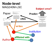
2.1 MAG240M: Node-Level Prediction
Practical relevance and dataset overview. The volume of scientific publication has been increasing exponentially, doubling every 12 years (Dong et al., 2017). Currently, subject areas of arXiv papers are manually determined by the paper’s authors and arXiv moderators. An accurate automatic predictor of papers’ subject categories not only reduces the significant burden of manual labeling, but can also be used to classify the vast number of non-arXiv papers, thereby allowing better search and organization of academic papers.
MAG240M is a heterogeneous academic graph extracted from the Microsoft Academic Graph (MAG) (Wang et al., 2020). Given arXiv papers situated in the heterogeneous graph, whose schema diagram is illustrated in Figure 2, we aim to automatically annotate their topics, i.e., predicting the primary subject area of each arXiv paper.
Graph. We extract 121M academic papers in English from MAG (version: 2020-11-23) to construct a heterogeneous academic graph. The resultant paper set is written by 122M author entities, who are affiliated with 26K institutes. Among these papers, there are 1.3 billion citation links captured by MAG. Each paper is associated with its natural language title and most papers’ abstracts are also available. We concatenate the title and abstract by period and pass it to a RoBERTa sentence encoder (Liu et al., 2019; Reimers and Gurevych, 2019), generating a 768-dimensional vector for each paper node. Among the 121M paper nodes, approximately 1.4M nodes are arXiv papers annotated with 153 arXiv subject areas, e.g., cs.LG (Machine Learning). On the paper nodes, we attach the publication years as meta information.
Prediction task and evaluation metric. The task is to predict the primary subject areas of the given arXiv papers, which is cast as an ordinary multi-class classification problem. The metric is the classification accuracy.
To understand the relation between the prediction task and the heterogeneous graph structure, we analyze the graph homophily (McPherson et al., 2001)—tendency of two adjacent nodes to share the same labels—to better understand the interplay between heterogeneous graph connectivity and the prediction task. Homophily is normally analyzed over a homogeneous graph, but we extend the analysis to the heterogenous graph by considering meta-paths (Sun et al., 2011)—a path consisting of a sequence of relations defined between different node types. Given a meta-path, we can say two nodes are adjacent if they are connected by the meta-path. Table 3 shows the homophily for different kinds of meta-paths with different levels of connection strength. Compared to the direct citation connection (i.e., P-P), certain meta-paths (i.e., P-A-P) give rise to much higher degrees of homophiliness, while other meta-paths (i.e., P-A-I-A-P) provide much less homophily. As homophily is the central graph property exploited by many graph ML models, we believe that discovering essential heterogeneous connectivity is important to achieve good performance on this dataset.
Dataset split. We split the data according to time. Specifically, we train models on arXiv papers published until 2018, validate the performance on the 2019 papers, and finally test the performance on the 2020 papers. The split reflects the practical scenario of helping the authors and moderators annotate the subject areas of the newly-published arXiv papers.
Baseline. We benchmark a broad range of graph ML models in both homogeneous (where only paper to paper relations are considered) and full heterogeneous settings. For both settings, we convert the directed graph into an undirected graph for simplicity. First, for the homogeneous setting, we benchmark the simple baseline models: graph-agnostic MLP, Label Propagation, and the recently-proposed simplified graph methods: SGC (Wu et al., 2019), SIGN (Rossi et al., 2020) and MLP+C&S (Huang et al., 2020), which are inherently scalable by decoupling predictions from propagation. Furthermore, we benchmark state-of-the-art expressive GNNs trained with neighborhood sampling (NS) (Hamilton et al., 2017), where we recursively sample 25 neighbors in the first layer and 15 neighbors in the second layer during training time. At inference time, we sample at most 160 neighbors for each layer. Here, we benchmark two types of strong models: the GraphSAGE (Hamilton et al., 2017) model (performing mean aggregation and utilizing skip-connections), and the more advanced Graph Attention Network (GAT) model (Velickovic et al., 2018). For the full heterogeneous setting, we follow Schlichtkrull et al. (2018) and learn distinct weights for each individual relation type (denoted by R-GraphSAGE and R-GAT, where “R” stands for “Relational”). We obtain the input features of authors and institutions by averaging the features of papers belonging to the same author and institution, respectively. The models are trained with NS. We note that the expressive GNNs trained with NS require more efforts to scale up, but are more expressive than the simple baselines.
Hyper-parameters. Hyper-parameters are selected based on their best validation performance. For all the models without NS, we tuned the hidden dimensionality , MLP depth , dropout ratio , propagation layers (for SGC, SIGN, and C&S) . For all the GNN models with NS, we use a hidden dimensionality of 1024. We make use of batch normalization (Ioffe and Szegedy, 2015) and ReLU activation in all models.
Discussion. Validation and test performances of all models considered are shown in Table 2. First, the graph-agnostic MLP and Label Propagation algorithm perform poorly, indicating that both graph structure and feature information are indeed important for the given task. Across the graph ML models operating on the homogeneous paper graph, GNNs with NS perform the best, with slight gains compared to their simplified versions. In particular, the advanced expressive graph attention aggregation is favourable compared to the uniform mean aggregation in GraphSAGE. Furthermore, considering all available heterogeneous relational structure in the heterogeneous graph setting yields significant improvements, with performance gains up to 3 percentage points. Again, the advanced attention aggregation provides favorable performance. Overall, our experiments highlight the benefits of developing and evaluating advanced expressive models on the larger scale.
KDD Cup 2021 summary. In Table 2, we show the results of the top 3 winners of the KDD Cup: BD-PGL Team (Shi et al., 2021), Academic Team (Addanki et al., 2021), and Synerise AI Team (Daniluk et al., 2021). All the solutions outperform our baselines significantly, yielding 5–6% gain in test accuracy. For a more direct comparison, with a single model (no model ensembling), the BD-PGL Team reports a validation accuracy of 73.71% (Shi et al., 2021), improving our best R-GAT baseline by 3.7%.
Notably, all the winning solutions used the target labels as input to their models, which allows the models to propagate labels together with the features. Regarding the GNN architectures, the BD-PGL adopted the expressive Transformer-based UniMP architecture (Shi et al., 2020), while the Academic adopted the standard MPNN (Gilmer et al., 2017) but trained it with self-supervised contrastive learning on unlabeled paper nodes (Thakoor et al., 2021). These results suggest that expressive GNNs are indeed promising for this dataset. Finally, both the BD-PGL and Academic teams exploited the temporal aspect of the academic graph by using the publication years either as input positional encoding (Shi et al., 2021) or as a way to sample mini-batch subgraphs for GNNs (Addanki et al., 2021). As real-world large-scale graphs are almost always dynamic, exploiting the temporal information is a promising direction of future research.

| Model | #Params | Validation | Test |
| MLP | 0.5M | 52.67 | 52.73 |
| LabelProp | 0 | 58.44 | 56.29 |
| SGC | 0.7M | 65.82 | 65.29 |
| SIGN | 3.8M | 66.64 | 66.09 |
| MLP+C&S | 0.5M | 66.98 | 66.18 |
| GraphSAGE (NS) | 4.9M | 66.79 | 66.28 |
| GAT (NS) | 4.9M | 67.15 | 66.80 |
| R-GraphSAGE (NS) | 12.2M | 69.86 | 68.94 |
| R-GAT (NS) | 12.3M | 70.02 | 69.42 |
| KDD 1st: BD-PGL | 75.49 | ||
| KDD 2nd: Academic | 75.19 | ||
| KDD 3rd: Synerise AI | 74.60 | ||
| Meta-path | Connect. | Homophily | #Edges |
| strength | ratio (%) | ||
| P-P | 1 | 57.80 | 2,017,844 |
| P-A-P | 1 | 46.12 | 88,099,071 |
| 2 | 57.02 | 12,557,765 | |
| 4 | 64.03 | 1,970,761 | |
| 8 | 66.65 | 476,792 | |
| 16 | 70.46 | 189,493 | |
| P-A-I-A-P | 1 | 3.83 | 159,884,165,669 |
| 2 | 4.61 | 81,949,449,717 | |
| 4 | 5.69 | 33,764,809,381 | |
| 8 | 6.85 | 12,390,929,118 | |
| 16 | 7.70 | 4,471,932,097 | |
| All pairs | 0 | 1.99 | 782,926,523,470 |
2.2 WikiKG90M: Link-Level Prediction
Practical relevance and dataset overview. Large encyclopedic Knowledge Graphs (KGs), such as Wikidata (Vrandečić and Krötzsch, 2014) and Freebase (Bollacker et al., 2008), represent factual knowledge about the world through triplets connecting different entities, e.g., Hinton Canada. They provide rich structured information about many entities, aiding a variety of knowledge-intensive downstream applications such as information retrieval, question answering (Singhal, 2012), and recommender systems (Guo et al., 2020). However, these large KGs are known to be far from complete (Min et al., 2013), missing many relational information between entities.
WikiKG90M is a Knowledge Graph (KG) extracted from the entire Wikidata knowledge base. The task is to automatically impute missing triplets that are not yet present in the current KG. Accurate imputation models can be readily deployed on the Wikidata to improve its coverage.
Graph. Each triplet (head, relation, tail) in WikiKG90M represents an Wikidata claim, where head and tail are the Wikidata items, and relation is the Wikidata predicate. We extracted triplets from the public Wikidata dump downloaded at three time-stamps: September 28, October 26, and November 23 of 2020, for training, validation, and testing, respectively. We retain all the entities and relations in the September dump, resulting in 87,143,637 entities, 1,315 relations, and 504,220,369 triplets in total.
In addition to extracting triplets, we provide text features for entities and relations. Specifically, each entity/relation in Wikidata is associated with a title and a short description, e.g., one entity is associated with the title ‘Geoffrey Hinton‘ and the description ‘computer scientist and psychologist‘. Similar to MAG240M, we provide RoBERTa embeddings (Reimers and Gurevych, 2019; Liu et al., 2019) as node and edge features.333We concatenate the title and description with comma, e.g., ‘Geoffrey Hinton, computer scientist and psychologist‘, and pass the sentence to a RoBERTa sentence encoder (Note that the RoBERTa model was trained before September 2020, so there is no obvious information leak). The title or/and description are sometimes missing, in which case we simply use the blank sentence to replace it.
Prediction task and evaluation metric. The task is the KG completion, i.e., given a set of training triplets, predict a set of test triplets. For evaluation, we follow the protocol similar to how KG completion is evaluated (Bordes et al., 2013). Specifically, for each validation/test triplet, (head, relation, tail), we corrupt tail with randomly-sampled 1000 negative entities, e.g., tail_neg, such that (head, relation, tail_neg) does not appear in the train/validation/test KG. The model is asked to rank the 1001 candidates (consisting of 1 positive and 1000 negatives) for each triplet and predict the top 10 entities that are most likely to be positive. The goal is to rank the ground-truth positive entity as high in the rank as possible, which is measured by Mean Reciprocal Rank (MRR). 444Note that this is more strict than the standard MRR since there is no partial score for positive entities being ranked outside of top 10.
Dataset split. We split the triplets according to time, simulating a realistic KG completion scenario of imputing missing triplets not present at a certain timestamp. Specifically, we construct three KGs using the aforementioned September, October, and November KGs, where we only retain entities and relation types that appear in the earliest September KG. We use the triplets in the September KG for training, and use the additional triplets in the October and November KGs for validation and test, respectively.
We analyze the effect of the time split. We find that head entities of validation triplets tend to be less popular entities; on average, they only have 6.5 out-degrees in the training KG, which is less than a quarter of the out-degree averaged over training triplets (i.e., 28.0). This suggests that learning signals for predicting validation (and test) triplets are sparse. Nonetheless, even for the sparsely-connected triplets, we find the textual information provides important clues, as illustrated in Table 4. Hence, we expect that advanced graph models that effectively incorporate textual information will be key to achieve good performance on the challenging time split.
Baseline. We consider two representative KG embedding models: TransE (Bordes et al., 2013) and ComplEx (Trouillon et al., 2016). These models define their own decoders to score knowledge triplets using the corresponding entity and relation embeddings. For instance, TransE uses as the decoder, where , , and are embeddings of head, relation, and tail, respectively. For the encoder function (mapping each entity and relation to its embedding), we consider the following three options. Shallow: We use the distinct embedding for each entity and relation, as normally done in KG embedding models. RoBERTa: We use two MLP encoders (one for entity and another for relation) that transform the RoBERTa features into entity and relation embeddings. Concat: To enhance the expressive power of the previous encoder, we concatenate the shallow learnable embeddings into the RoBERTa features, and use the MLPs to transform the concatenated vectors to get the final embeddings. This way, the MLP encoders can adaptively utilize the RoBERTa features and the shallow embeddings to fit the large amount of triplet data. To implement our baselines, we utilize DGL-KE (Zheng et al., 2020).
Hyper-parameters. For the loss function, we use the negative sampling loss from Sun et al. (2019), where we pick margin from {1,4,8,10,100}. In order to balance the performance and the memory cost, we use the embedding dimensionality of 200 for all the models.
Discussion. Table 5 shows the validation and test performance of the six different models, i.e., combination of two decoders (TransE and ComplEx) and three encoders (Shallow, RoBERTa, and Concat). Notably, in terms of the encoders, we see that the most expressive Concat outperforms both Shallow and RoBERTa, indicating that both the textual information (captured by the RoBERTa embeddings) and structural information (captured by node-wise learnable embeddings) are useful in predicting validation and test triplets. In terms of the decoders, TransE and ComplEx show similar performance with the Concat encoder, while they show somewhat mixed results with the Shallow and RoBERTa encoders.
Overall, our experiments suggest that the expressive encoder that combines both textual information and structural information gives the most promising performance. In the KG completion literature, the design of the encoder has been much less studied compared to the decoder designs. Therefore, we believe there is a huge opportunity in scaling up more advanced encoders, especially GNNs (Schlichtkrull et al., 2018), to further improve the performance on this dataset.
KDD Cup 2021 summary. Table 5 shows the results of the top 3 winners of the KDD Cup: BD-PGL Team (Su et al., 2021), OhMyGod Team (Peng et al., 2021), and the GraphMIRAcles Team (Cai et al., 2021). All the winning solutions outperform our strong baselines significantly, achieving near-perfect test MRR score of 0.97. For a more direct comparison, with a single model (no model ensembling), the BD-PGL Team reports a validation MRR of 0.92 (Su et al., 2021), improving our best ComplEx-Concat baseline by 0.07 points in validation MRR. Similar to our baselines, all the winners utilize the KG embedding approach as the backbone, and adopt the encoder that takes both shallow embedding and textual embeddings into account. Specifically, BD-PGL proposed the NOTE model (Su et al., 2021) which makes the RotatE model more expressive, while OhMyGod adopted the ensemble of several existing KG embedding models. On the other hand, GraphMIRAcles explored different design choices for the encoder and found that adding residual connection for shallow embeddings significantly improved the model performance.
In addition to the model advances, all the winners exploited some statistical property of candidate tail entities. Most notably, Yang et al. (2021) found that simply by sorting the candidate tails by the frequency they appear in the training KG, it was possible to achieve validation MRR of 0.75, rivaling our TransE-Shallow baseline. This highlights that our negative tail candidates are mostly rare entities that can be easily distinguished from the true tail entity. On the other hand, the practical KG completion presents a much harder challenge: the candidate tails are not provided, and a model needs to predict the true tail entity out of all the possible 87M entities. As the performance on WikiKG90M has already saturated, we have updated WikiKG90M to WikiKG90Mv2 to reflect the realistic setting in large-scale KG completion. See Section 3 for further details.
| Head | Relation | Tail |
| Food and drink companies of Bulgaria | combines topics | Bulgaria |
| Performing arts in Denmark | combines topics | performing arts |
| Anglicanism in Grenada | combines topics | Anglicanism |
| Chuan Li | occupation | researcher |
| Petra Junkova | given name | Petra |
| Model | #Params | Validation | Test |
| TransE-Shallow | 17.4B | 0.7559 | 0.7412 |
| ComplEx-Shallow | 17.4B | 0.6142 | 0.5883 |
| TransE-RoBERTa | 0.3M | 0.6039 | 0.6288 |
| ComplEx-RoBERTa | 0.3M | 0.7052 | 0.7186 |
| TransE-Concat | 17.4B | 0.8494 | 0.8548 |
| ComplEx-Concat | 17.4B | 0.8425 | 0.8637 |
| KDD 1st: BD-PGL | 0.9727 | ||
| KDD 2nd: OhMyGod | 0.9712 | ||
| KDD 3rd: GraphMIRAcles | 0.9707 | ||
2.3 PCQM4M: Graph-Level Prediction
Practical relevance and dataset overview. Density Functional Theory (DFT) is a powerful and widely-used quantum physics calculation that can accurately predict various molecular properties such as the shape of molecules, reactivity, responses by electromagnetic fields (Burke, 2012). However, DFT is time-consuming and takes up to several hours per small molecule. Using fast and accurate ML models to approximate DFT enables diverse downstream applications, such as property prediction for organic photovaltaic devices (Cao and Xue, 2014) and structure-based virtual screening for drug discovery (Ferreira et al., 2015).
PCQM4M is a quantum chemistry dataset originally curated under the PubChemQC project (Nakata, 2015; Nakata and Shimazaki, 2017). Based on the PubChemQC, we define a meaningful ML task of predicting DFT-calculated HOMO-LUMO energy gap of molecules given their 2D molecular graphs. The HOMO-LUMO gap is one of the most practically-relevant quantum chemical properties of molecules since it is related to reactivity, photoexcitation, and charge transport (Griffith and Orgel, 1957). Moreover, predicting the quantum chemical property only from 2D molecular graphs without their 3D equilibrium structures is also practically favorable. This is because obtaining 3D equilibrium structures requires DFT-based geometry optimization, which is expensive on its own.
To ensure the resulting models are practically useful, we limit the average inference budget per molecule (including both pre-processing and model inference) to be less than 0.1 second using a single GPU and CPU (multi-threading on a multi-core CPU is allowed). This means that expensive (quantum) calculations cannot be used to perform inference. As our test set contains 377,423 molecules, we require the all the prediction to be made within 12 hours. Note that this time constraint is quite generous for ordinary GNNs—each of our baseline GNN only took about 3 minutes to perform inference over the entire test data.
Graph. We provide molecules as the SMILES strings (Weininger, 1988), from which 2D molecule graphs (nodes are atoms and edges are chemical bonds) as well as molecular fingerprints (hand-engineered molecular feature developed by the chemistry community) can be obtained. By default, we follow OGB (Hu et al., 2020a) to convert the SMILES string into a molecular graph representation, where each node is associated with a 9-dimensional feature (e.g., atomic number, chirality) and each edge comes with a 3-dimensional feature (e.g., bond type, bond stereochemistry), although the optimal set of input graph features remains to be explored.
Prediction task and evaluation metric. The task is graph regression: predicting the HOMO-LUMO energy gap in electronvolt (eV) given 2D molecular graphs. Mean Absolute Error (MAE) is used as evaluation metric.
Dataset split. We split molecules by their PubChem ID (CID) with ratio 80/10/10. Our original intention was to provide the scaffold split (Hu et al., 2020a; Wu et al., 2018), but the provided data turns out to be split by the CID due to some pre-processing bug. The CID number itself does not indicate particular meaning about the molecule, but splitting by CID may provide a moderate distribution shift (most likely not as severe as the scaffold split). We empirically compared the CID and scaffold splits and found the model performances were consistent between the two splits.555Detailed discussion can be found at https://github.com/snap-stanford/ogb/discussions/162
Baseline. We benchmark two types of models: a simple MLP over the Morgan fingerprint (Morgan, 1965) and more advanced GNN models. For GNNs, we use the four strong models developed for graph-level prediction: Graph Convolutional Network (GCN) (Kipf and Welling, 2017) and Graph Isomorphism Network (GIN) (Xu et al., 2019), as well as their variants, GCN-virtual and GIN-virtual, which augment graphs with a virtual node that is bidirectionally connected to all nodes in the original graph (Gilmer et al., 2017). Adding the virtual node is shown to be effective across a wide range of graph-level prediction datasets in OGB (Hu et al., 2020a). Edge features are incorporated following Hu et al. (2020b). At inference time, the model output is clamped between 0 and 50 to avoid model’s anomalously large/small prediction.
Hyper-parameters. For the MLP over Morgan fingerprint, we set the fingerprint dimensionality to be 2048, and tune the fingerprint radius , as well as MLP’s hyper-parameters: hidden dimensionality , number of hidden layers , and dropout ratio . For GNNs, we tune hidden dimensionality, i.e., width , number of GNN layers, i.e., depth . Simple summation is used for graph-level pooling. For all MLPs (including GIN’s), we use batch normalization (Ioffe and Szegedy, 2015) and ReLU activation.
Discussion. The validation and test results are shown in Table 6. We see both the GNN models significantly outperform the simple fingerprint baseline. Expressive GNNs (GIN and GIN-virtual) outperform less expressive ones (GCN and GCN-virtual); especially, the most advanced and expressive GIN-virtual model significantly outperforms the other GNNs. Nonetheless, the current performance is still much worse than the chemical accuracy of 0.043eV—an indicator of practical usefulness established by the chemistry community. In the same Table 6, we show our ablation, where we use only 10% of data to train the GIN-virtual model. We see the performance significantly deteriorate, indicating the importance of training the model on large data. Finally, in Table 7, we show the relation between model sizes and validation performance. We see that the largest models always achieve the best performance.
Overall, we find that advanced, expressive, and large GNN model gives the most promising performance on the PCQM4M dataset, although the performance still needs to be improved for practical use. We believe further advances in advanced modeling, expressive architectures, and larger model sizes could yield breakthrough in the large-scale molecular property prediction task.
KDD Cup 2021 summary. In Table 6, we show the results of the top 3 winners of the KDD Cup: Machine Learning Team (Ying et al., 2021b), SuperHelix Team (Zhang et al., 2021), and Quantum Team (Addanki et al., 2021). The winners have significantly reduced the MAE compared our baselines, yielding around 0.03 points improvement in test MAE. For a more direct comparison, with a single model, the Machine Learning reports the validation MAE of 0.097 for their Graphormer model (Ying et al., 2021a), which is 0.04 points lower than our best GIN-virtual baseline.
In terms of methodology, we find that the winning solutions share three important components in common. (1) Their winning GNN models are indeed large and deep; the number of learnable parameters (single model) ranges from 50M up to 450M, while the number of GNN layers ranges from 11 up to 50, being significantly larger than our baseline models. (2) All the GNNs perform global message passing at each layer, either through the virtual nodes (Gilmer et al., 2017) or fully-connected Transformer-style self-attention (Ying et al., 2021a). (3) All the winners utilize 3D structure of molecules to supervise their GNNs. As 3D structure was not provided at our KDD Cup, the winners generate the 3D structure themselves using RDkit (Landrum et al., 2006) or PySCF (Sun et al., 2020), both of which provide cheap but less accurate 3D structure of molecules.
As modeling 3D molecular graphs is a promising direction in graph ML (Schütt et al., 2017; Klicpera et al., 2020; Sanchez-Gonzalez et al., 2020; Hu et al., 2021), we have updated PCQM4M to PCQM4Mv2 to include DFT-calculated 3D structures for training molecules. Details are provided in Section 3.
| Model | #Params | Validation | Test |
| MLP-fingerprint | 16.1M | 0.2044 | 0.2070 |
| GCN | 2.0M | 0.1684 | 0.1842 |
| GCN-virtual | 4.9M | 0.1510 | 0.1580 |
| GIN | 3.8M | 0.1536 | 0.1685 |
| GIN-virtual | 6.7M | 0.1396 | 0.1494 |
| MLP-fingerprint (10% train) | 6.8M | 0.2708 | 0.2659 |
| GIN-virtual (10% train) | 6.7M | 0.1790 | 0.1892 |
| KDD 1st: MachineLearning | 0.1208 | ||
| KDD 2nd: SuperHelix | 0.1210 | ||
| KDD 3rd: Quantum | 0.1211 | ||
| Chemical accuracy (goal) | – | 0.0430 | |
| Model | Width | Depth | #Params | Validation |
| MLP-fingerprint | 1600 | 6 | 16.1M | 0.2044 |
| 1600 | 4 | 11.0M | 0.2044 | |
| 1600 | 2 | 5.8M | 0.2220 | |
| 1200 | 6 | 9.7M | 0.2083 | |
| GIN-virtual | 600 | 5 | 6.7M | 0.1410 |
| 600 | 3 | 3.7M | 0.1462 | |
| 300 | 5 | 1.7M | 0.1442 | |
| 300 | 3 | 1.0M | 0.1512 |
3 Updates after the KDD Cup
To facilitate further research advances, we have updated the datasets and leaderboards based on the lessons learned from our KDD Cup 2021. Here we briefly describe our updates. More details are provided in Appendix C.
Updates on WikiKG90M.
From the KDD Cup results, we learned that most of our provided negative entities in the large-scale WikiKG90M are “easy negatives”, and our current task gives overly-optimistic performance scores. In a realistic large-scale KG completion setting, ML models are required to predict the true tail entity from nearly 90M entities, which is much more challenging. To reflect this challenge, we have updated WikiKG90M to WikiKG90Mv2, where we do not provide any candidate entities for validation/test triples. Our initial experiments using the same set of baseline models, shows that WikiKG90Mv2 indeed provides a much harder challenge; our best model ComplEx-Concat only achieves 0.1833 MRR on WikiKG90Mv2 as opposed to achieving 0.8637 MRR on WikiKG90M, leaving significant room for further improvement.
Updates on PCQM4M.
From the KDD Cup results, we saw that the winners effectively utilized (self-calculated) 3D structure of molecules. Modeling molecular graphs in 3D space is of great interest to the graph ML community; We therefore have updated PCQM4M to PCQM4Mv2, where we provide DFT-calculated 3D structure for training molecules. For validation and test molecules, 3D structures is not be provided, and ML models still need to make prediction based on the 2D molecular graphs. In updating to PCQM4Mv2, we are also fixing subtle but important mismatch between some of the 2D molecular graphs and the corresponding 3D molecular graphs. Our preliminary experiments on PCQM4Mv2 suggest that the all the baseline models’ MAE is improved by [eV] compared to PCQM4M, although the trends in model performance stay almost the same as PCQM4M.
Updates on leaderboards.
We are introducing public leaderboards to facilitate further research advances after our KDD Cup. The test submissions of the KDD Cup 2021 were evaluated on the entire hidden test set. After the KDD Cup, we are randomly splitting the test set into two: “test-dev” and “test-challenge”. The test-dev set is be used for public leaderboards that evaluate test submissions any time during a year. The test-challenge set is be left for future competitions, which we plan to hold annually to facilitate community engagement. The leaderboards have been released together with the updated datasets.
4 Conclusions
Modern applications of graph ML involve large-scale graph data with billions of edges or millions of graphs. ML advances on large graph data have been limited due to the lack of a suitable benchmark. Here we present OGB-LSC, with the goal of advancing state-of-the-art in large-scale graph ML. OGB-LSC provides the three large-scale realistic benchmark datasets, covering the core graph ML tasks of node classification, link prediction, and graph regression. We perform dedicated baseline analysis, scaling up advanced graph models to large graphs. We show that advanced and expressive models can significantly outperform simpler baseline models, suggesting opportunities for further dedicated effort to yield even better performance.
We used our datasets for the recent ACM KDD Cup 2021, where we have attracted huge engagement from the community and have already witnessed significant performance improvement. We summarize the winning solutions for each dataset, highliting the current best practices in large-scale graph ML. Finally, we describe how we have updated our datasets after the KDD Cup to further facilitate research advances. Overall, we hope OGB-LSC encourages dedicated community efforts to tackle the important but challenging problem of large-scale graph ML.
Acknowledgement
We thank Michele Catasta and Larry Zitnick for helpful discussion, Shigeru Maya for motivating the project, Adrijan Bradaschia for setting up the server for the project, and Amit Bleiweiss, Benjamin Braun and Hanjun Dai for providing helpful feedback on our baseline code, and the DGL Team for hosting our large datasets.
Stanford University is supported by DARPA under Nos. N660011924033 (MCS); ARO under Nos. W911NF-16-1-0342 (MURI), W911NF-16-1-0171 (DURIP); NSF under Nos. OAC-1835598 (CINES), OAC-1934578 (HDR), CCF-1918940 (Expeditions), IIS-2030477 (RAPID); Stanford Data Science Initiative, Wu Tsai Neurosciences Institute, Chan Zuckerberg Biohub, Amazon, JPMorgan Chase, Docomo, Hitachi, JD.com, KDDI, NVIDIA, Dell, Toshiba, Intel, and UnitedHealth Group. Weihua Hu is supported by Funai Overseas Scholarship and Masason Foundation Fellowship. Matthias Fey is supported by the German Research Association (DFG) within the Collaborative Research Center SFB 876 “Providing Information by Resource-Constrained Analysis”, project A6. Hongyu Ren is supported by Masason Foundation Fellowship and Apple PhD Fellowship. Jure Leskovec is a Chan Zuckerberg Biohub investigator.
Our baseline code and Python package are built on top of excellent open-source software, including Numpy (Harris et al., 2020), Pytorch (Paszke et al., 2017), Pytorch Geometric (Fey and Lenssen, 2019), DGL (Wang et al., 2019), and DGL-KE (Zheng et al., 2020).
The HOKUSAI facility was used to perform some of the quantum calculations. This work was supported by the Japan Society for the Promotion of Science (JSPS KAKENHI Grant no. 18H03206). We are also grateful to Maeda Toshiyuki for helpful discussions.
References
- Addanki et al. (2021) Ravichandra Addanki, Peter W Battaglia, David Budden, Andreea Deac, Jonathan Godwin, Thomas Keck, Wai Lok Sibon Li, Alvaro Sanchez-Gonzalez, Jacklynn Stott, Shantanu Thakoor, et al. Large-scale graph representation learning with very deep gnns and self-supervision. arXiv preprint arXiv:2107.09422, 2021.
- Bollacker et al. (2008) Kurt Bollacker, Colin Evans, Praveen Paritosh, Tim Sturge, and Jamie Taylor. Freebase: a collaboratively created graph database for structuring human knowledge. In Special Interest Group on Management of Data (SIGMOD), pages 1247–1250. AcM, 2008.
- Bordes et al. (2013) Antoine Bordes, Nicolas Usunier, Alberto Garcia-Duran, Jason Weston, and Oksana Yakhnenko. Translating embeddings for modeling multi-relational data. In Advances in Neural Information Processing Systems (NeurIPS), pages 2787–2795, 2013.
- Brown et al. (2020) Tom B Brown, Benjamin Mann, Nick Ryder, Melanie Subbiah, Jared Kaplan, Prafulla Dhariwal, Arvind Neelakantan, Pranav Shyam, Girish Sastry, Amanda Askell, et al. Language models are few-shot learners. arXiv preprint arXiv:2005.14165, 2020.
- Burke (2012) K. Burke. Perspective on density functional theory. J. Chem. Phys., 136:150901, 2012. URL http://link.aip.org/link/doi/10.1063/1.4704546.
- Cai et al. (2021) Jianyu Cai, Jiajun Chen, Taoxing Pan, Zhanqiu Zhang, and Jie Wang. Technical report of team graphmiracles in the wikikg90m-lsc track of ogb-lsc@ kdd cup 2021. 2021.
- Cao and Xue (2014) Weiran Cao and Jiangeng Xue. Recent progress in organic photovoltaics: Device architecture and optical design. Energy Environ. Sci., 7:2123–2144, 2014. doi: 10.1039/C4EE00260A. URL http://dx.doi.org/10.1039/C4EE00260A.
- Chanussot et al. (2021) Lowik Chanussot, Abhishek Das, Siddharth Goyal, Thibaut Lavril, Muhammed Shuaibi, Morgane Riviere, Kevin Tran, Javier Heras-Domingo, Caleb Ho, Weihua Hu, Aini Palizhati, Anuroop Sriram, Brandon Wood, Junwoong Yoon, Devi Parikh, C. Lawrence Zitnick, and Zachary Ulissi. Open catalyst 2020 (oc20) dataset and community challenges. ACS Catal., 11:6059–6072, 2021. URL https://doi.org/10.1021/acscatal.0c04525.
- Chen et al. (2018) Jie Chen, Tengfei Ma, and Cao Xiao. Fastgcn: fast learning with graph convolutional networks via importance sampling. arXiv preprint arXiv:1801.10247, 2018.
- Chiang et al. (2019) Wei-Lin Chiang, Xuanqing Liu, Si Si, Yang Li, Samy Bengio, and Cho-Jui Hsieh. Cluster-GCN: An efficient algorithm for training deep and large graph convolutional networks. In ACM SIGKDD Conference on Knowledge Discovery and Data Mining (KDD), pages 257–266, 2019.
- Daniluk et al. (2021) Michał Daniluk, Jacek Dabrowski, Barbara Rychalska, and Konrad Gołuchowski. Synerise at kdd cup 2021: Node classification in massive heterogeneous graphs. 2021. URL https://ogb.stanford.edu/paper/kddcup2021/mag240m_SyneriseAI.pdf.
- Devlin et al. (2018) Jacob Devlin, Ming-Wei Chang, Kenton Lee, and Kristina Toutanova. Bert: Pre-training of deep bidirectional transformers for language understanding. arXiv preprint arXiv:1810.04805, 2018.
- Dong et al. (2017) Yuxiao Dong, Hao Ma, Zhihong Shen, and Kuansan Wang. A century of science: Globalization of scientific collaborations, citations, and innovations. In ACM SIGKDD Conference on Knowledge Discovery and Data Mining (KDD), pages 1437–1446. ACM, 2017.
- Ferreira et al. (2015) Leonardo G. Ferreira, Ricardo N. Dos Santos, Glaucius Oliva, and Adriano D. Andricopulo. Molecular docking and structure-based drug design strategies. Molecules, 20(7):13384–13421, 2015. ISSN 1420-3049. doi: 10.3390/molecules200713384. URL https://www.mdpi.com/1420-3049/20/7/13384.
- Fey and Lenssen (2019) Matthias Fey and Jan Eric Lenssen. Fast graph representation learning with pytorch geometric. arXiv preprint arXiv:1903.02428, 2019.
- Gilmer et al. (2017) Justin Gilmer, Samuel S Schoenholz, Patrick F Riley, Oriol Vinyals, and George E Dahl. Neural message passing for quantum chemistry. In International Conference on Machine Learning (ICML), pages 1273–1272, 2017.
- Griffith and Orgel (1957) JS Griffith and LE Orgel. Ligand-field theory. Quarterly Reviews, Chemical Society, 11(4):381–393, 1957.
- Guo et al. (2020) Qingyu Guo, Fuzhen Zhuang, Chuan Qin, Hengshu Zhu, Xing Xie, Hui Xiong, and Qing He. A survey on knowledge graph-based recommender systems. IEEE Transactions on Knowledge and Data Engineering, 2020.
- Hamilton et al. (2017) William L Hamilton, Rex Ying, and Jure Leskovec. Inductive representation learning on large graphs. In Advances in Neural Information Processing Systems (NeurIPS), pages 1025–1035, 2017.
- Harris et al. (2020) Charles R Harris, K Jarrod Millman, Stéfan J van der Walt, Ralf Gommers, Pauli Virtanen, David Cournapeau, Eric Wieser, Julian Taylor, Sebastian Berg, Nathaniel J Smith, et al. Array programming with numpy. Nature, 585(7825):357–362, 2020.
- He et al. (2016) Kaiming He, Xiangyu Zhang, Shaoqing Ren, and Jian Sun. Deep residual learning for image recognition. In IEEE Conference on Computer Vision and Pattern Recognition (CVPR), pages 770–778, 2016.
- Hu et al. (2020a) Weihua Hu, Matthias Fey, Marinka Zitnik, Yuxiao Dong, Hongyu Ren, Bowen Liu, Michele Catasta, and Jure Leskovec. Open graph benchmark: Datasets for machine learning on graphs. In Advances in Neural Information Processing Systems (NeurIPS), 2020a.
- Hu et al. (2020b) Weihua Hu, Bowen Liu, Joseph Gomes, Marinka Zitnik, Percy Liang, Vijay Pande, and Jure Leskovec. Strategies for pre-training graph neural networks. In International Conference on Learning Representations (ICLR), 2020b.
- Hu et al. (2021) Weihua Hu, Muhammed Shuaibi, Abhishek Das, Siddharth Goyal, Anuroop Sriram, Jure Leskovec, Devi Parikh, and C Lawrence Zitnick. Forcenet: A graph neural network for large-scale quantum calculations. arXiv preprint arXiv:2103.01436, 2021.
- Huang et al. (2020) Qian Huang, Horace He, Abhay Singh, Ser-Nam Lim, and Austin R Benson. Combining label propagation and simple models out-performs graph neural networks. arXiv preprint arXiv:2010.13993, 2020.
- Ioffe and Szegedy (2015) Sergey Ioffe and Christian Szegedy. Batch normalization: Accelerating deep network training by reducing internal covariate shift. In International Conference on Machine Learning (ICML), pages 448–456, 2015.
- Kipf and Welling (2017) Thomas N. Kipf and Max Welling. Semi-supervised classification with graph convolutional networks. In International Conference on Learning Representations (ICLR), 2017.
- Kleinberg (1999) Jon M Kleinberg. Authoritative sources in a hyperlinked environment. Journal of the ACM, 46(5):604–632, 1999.
- Klicpera et al. (2020) Johannes Klicpera, Shankari Giri, Johannes T. Margraf, and Stephan Günnemann. Fast and uncertainty-aware directional message passing for non-equilibrium molecules. In NeurIPS-W, 2020.
- Landrum et al. (2006) Greg Landrum et al. Rdkit: Open-source cheminformatics, 2006.
- Leskovec and Sosič (2016) Jure Leskovec and Rok Sosič. Snap: A general-purpose network analysis and graph-mining library. ACM Transactions on Intelligent Systems and Technology (TIST), 8(1):1–20, 2016.
- Lin et al. (2014) Tsung-Yi Lin, Michael Maire, Serge Belongie, James Hays, Pietro Perona, Deva Ramanan, Piotr Dollár, and C Lawrence Zitnick. Microsoft coco: Common objects in context. In eccv, pages 740–755. Springer, 2014.
- Liu et al. (2019) Yinhan Liu, Myle Ott, Naman Goyal, Jingfei Du, Mandar Joshi, Danqi Chen, Omer Levy, Mike Lewis, Luke Zettlemoyer, and Veselin Stoyanov. Roberta: A robustly optimized bert pretraining approach. arXiv preprint arXiv:1907.11692, 2019.
- McPherson et al. (2001) Miller McPherson, Lynn Smith-Lovin, and James M Cook. Birds of a feather: Homophily in social networks. Annual review of sociology, 27(1):415–444, 2001.
- Min et al. (2013) Bonan Min, Ralph Grishman, Li Wan, Chang Wang, and David Gondek. Distant supervision for relation extraction with an incomplete knowledge base. In North American Chapter of the Association for Computational Linguistics (NAACL), pages 777–782, 2013.
- Morgan (1965) Harry L Morgan. The generation of a unique machine description for chemical structures-a technique developed at chemical abstracts service. Journal of Chemical Documentation, 5(2):107–113, 1965.
- Morris et al. (2020) Christopher Morris, Nils M Kriege, Franka Bause, Kristian Kersting, Petra Mutzel, and Marion Neumann. Tudataset: A collection of benchmark datasets for learning with graphs. arXiv preprint arXiv:2007.08663, 2020.
- Nakata (2015) Maho Nakata. the PubChemQC Project: A Large Chemical Database from the First Principle Calculations. AIP Conf. Proc., 1702:090058, 2015. doi: 10.1186/1758-2946-3-4. URL http://dx.doi.org/10.1063/1.4938866.
- Nakata and Shimazaki (2017) Maho Nakata and Tomomi Shimazaki. Pubchemqc project: A large-scale first-principles electronic structure database for data-driven chemistry. Journal of chemical information and modeling, 57(6):1300–1308, 2017.
- Paszke et al. (2017) Adam Paszke, Sam Gross, Soumith Chintala, Gregory Chanan, Edward Yang, Zachary DeVito, Zeming Lin, Alban Desmaison, Luca Antiga, and Adam Lerer. Automatic differentiation in pytorch. In NIPS-W, 2017.
- Peng et al. (2021) Weihua Peng, Donghai Bian, Yanhui Huang, Guangzhi Sheng, and Jian Sun. Technical report of wikikg90m-lsc. 2021. URL https://ogb.stanford.edu/paper/kddcup2021/wikikg90m_OhMyGod.pdf.
- Reimers and Gurevych (2019) Nils Reimers and Iryna Gurevych. Sentence-bert: Sentence embeddings using siamese bert-networks. 11 2019. URL https://arxiv.org/abs/1908.10084.
- Rossi et al. (2020) Emanuele Rossi, Fabrizio Frasca, Ben Chamberlain, Davide Eynard, Michael Bronstein, and Federico Monti. Sign: Scalable inception graph neural networks. arXiv preprint arXiv:2004.11198, 2020.
- Russakovsky et al. (2015) Olga Russakovsky, Jia Deng, Hao Su, Jonathan Krause, Sanjeev Satheesh, Sean Ma, Zhiheng Huang, Andrej Karpathy, Aditya Khosla, Michael Bernstein, et al. Imagenet large scale visual recognition challenge. International journal of computer vision, 115(3):211–252, 2015.
- Sanchez-Gonzalez et al. (2020) Alvaro Sanchez-Gonzalez, Jonathan Godwin, Tobias Pfaff, Rex Ying, Jure Leskovec, and Peter W Battaglia. Learning to simulate complex physics with graph networks. In International Conference on Machine Learning (ICML), 2020.
- Schlichtkrull et al. (2018) Michael Schlichtkrull, Thomas N Kipf, Peter Bloem, Rianne Van Den Berg, Ivan Titov, and Max Welling. Modeling relational data with graph convolutional networks. In European Semantic Web Conference, pages 593–607. Springer, 2018.
- Schütt et al. (2017) Kristof Schütt, Pieter-Jan Kindermans, Huziel Enoc Sauceda Felix, Stefan Chmiela, Alexandre Tkatchenko, and Klaus-Robert Müller. Schnet: A continuous-filter convolutional neural network for modeling quantum interactions. In Advances in Neural Information Processing Systems (NeurIPS), pages 991–1001, 2017.
- Shi et al. (2020) Yunsheng Shi, Zhengjie Huang, Wenjin Wang, Hui Zhong, Shikun Feng, and Yu Sun. Masked label prediction: Unified message passing model for semi-supervised classification. arXiv preprint arXiv:2009.03509, 2020.
- Shi et al. (2021) Yunsheng Shi, PGL Team, Zhengjie Huang, Weibin Li, Weiyue Su, and Shikun Feng. Runimp: Solution for kddcup 2021 mag240m-lsc. 2021. URL https://ogb.stanford.edu/paper/kddcup2021/mag240m_BD-PGL.pdf.
- Singhal (2012) Amit Singhal. Introducing the knowledge graph: things, not strings. Official google blog, 5:16, 2012.
- Song et al. (2020) Kaitao Song, Xu Tan, Tao Qin, Jianfeng Lu, and Tie-Yan Liu. Mpnet: Masked and permuted pre-training for language understanding. arXiv preprint arXiv:2004.09297, 2020.
- Su et al. (2021) Weiyue Su, Zeyang Fang, Hui Zhong, Huijuan Wang, Siming Dai, Zhengjie Huang, Yunsheng Shi, Shikun Feng, and Zeyu Chen. Note: Solution for kdd-cup 2021 wikikg90m-lsc. arXiv preprint arXiv:2107.01892, 2021.
- Sun et al. (2020) Qiming Sun, Xing Zhang, Samragni Banerjee, Peng Bao, Marc Barbry, Nick S Blunt, Nikolay A Bogdanov, George H Booth, Jia Chen, Zhi-Hao Cui, et al. Recent developments in the pyscf program package. The Journal of chemical physics, 153(2):024109, 2020.
- Sun et al. (2011) Yizhou Sun, Jiawei Han, Xifeng Yan, Philip S Yu, and Tianyi Wu. Pathsim: Meta path-based top-k similarity search in heterogeneous information networks. Proceedings of the VLDB Endowment, 4(11):992–1003, 2011.
- Sun et al. (2019) Zhiqing Sun, Zhi-Hong Deng, Jian-Yun Nie, and Jian Tang. Rotate: Knowledge graph embedding by relational rotation in complex space. In International Conference on Learning Representations (ICLR), 2019.
- Thakoor et al. (2021) Shantanu Thakoor, Corentin Tallec, Mohammad Gheshlaghi Azar, Rémi Munos, Petar Veličković, and Michal Valko. Bootstrapped representation learning on graphs. arXiv preprint arXiv:2102.06514, 2021.
- Trouillon et al. (2016) Théo Trouillon, Johannes Welbl, Sebastian Riedel, Éric Gaussier, and Guillaume Bouchard. Complex embeddings for simple link prediction. In International Conference on Machine Learning (ICML), pages 2071–2080, 2016.
- Ugander et al. (2011) Johan Ugander, Brian Karrer, Lars Backstrom, and Cameron Marlow. The anatomy of the facebook social graph. arXiv preprint arXiv:1111.4503, 2011.
- Vaswani et al. (2017) Ashish Vaswani, Noam Shazeer, Niki Parmar, Jakob Uszkoreit, Llion Jones, Aidan N Gomez, Lukasz Kaiser, and Illia Polosukhin. Attention is all you need. arXiv preprint arXiv:1706.03762, 2017.
- Velickovic et al. (2018) Petar Velickovic, Guillem Cucurull, Arantxa Casanova, Adriana Romero, Pietro Lio, and Yoshua Bengio. Graph attention networks. In International Conference on Learning Representations (ICLR), 2018.
- Vrandečić and Krötzsch (2014) Denny Vrandečić and Markus Krötzsch. Wikidata: a free collaborative knowledgebase. Communications of the ACM, 57(10):78–85, 2014.
- Wang et al. (2018) Alex Wang, Amanpreet Singh, Julian Michael, Felix Hill, Omer Levy, and Samuel R Bowman. Glue: A multi-task benchmark and analysis platform for natural language understanding. arXiv preprint arXiv:1804.07461, 2018.
- Wang et al. (2020) Kuansan Wang, Zhihong Shen, Chiyuan Huang, Chieh-Han Wu, Yuxiao Dong, and Anshul Kanakia. Microsoft academic graph: When experts are not enough. Quantitative Science Studies, 1(1):396–413, 2020.
- Wang et al. (2019) Minjie Wang, Lingfan Yu, Da Zheng, Quan Gan, Yu Gai, Zihao Ye, Mufei Li, Jinjing Zhou, Qi Huang, Chao Ma, Ziyue Huang, Qipeng Guo, Hao Zhang, Haibin Lin, Junbo Zhao, Jinyang Li, Alexander J Smola, and Zheng Zhang. Deep graph library: Towards efficient and scalable deep learning on graphs. ICLR Workshop on Representation Learning on Graphs and Manifolds, 2019. URL https://arxiv.org/abs/1909.01315.
- Weininger (1988) David Weininger. Smiles, a chemical language and information system. 1. introduction to methodology and encoding rules. Journal of chemical information and computer sciences, 28(1):31–36, 1988.
- Wu et al. (2019) Felix Wu, Tianyi Zhang, Amauri Holanda de Souza Jr, Christopher Fifty, Tao Yu, and Kilian Q Weinberger. Simplifying graph convolutional networks. In International Conference on Machine Learning (ICML), 2019.
- Wu et al. (2018) Zhenqin Wu, Bharath Ramsundar, Evan N Feinberg, Joseph Gomes, Caleb Geniesse, Aneesh S Pappu, Karl Leswing, and Vijay Pande. Moleculenet: a benchmark for molecular machine learning. Chemical science, 9(2):513–530, 2018.
- Xu et al. (2019) Keyulu Xu, Weihua Hu, Jure Leskovec, and Stefanie Jegelka. How powerful are graph neural networks? In International Conference on Learning Representations (ICLR), 2019.
- Yang et al. (2021) Shuo Yang, Daixin Wang, Dingyuan Zhu, Yakun Wang, and Borui Ye. Team littleant’s solution of task2. 2021. URL https://ogb.stanford.edu/paper/kddcup2021/wikikg90m_littleant.pdf.
- Yang et al. (2016) Zhilin Yang, William W Cohen, and Ruslan Salakhutdinov. Revisiting semi-supervised learning with graph embeddings. In International Conference on Machine Learning (ICML), pages 40–48, 2016.
- Ying et al. (2021a) Chengxuan Ying, Tianle Cai, Shengjie Luo, Shuxin Zheng, Guolin Ke, Di He, Yanming Shen, and Tie-Yan Liu. Do transformers really perform bad for graph representation? arXiv preprint arXiv:2106.05234, 2021a.
- Ying et al. (2021b) Chengxuan Ying, Mingqi Yang, Shuxin Zheng, Guolin Ke, Shengjie Luo, Tianle Cai, Chenglin Wu, Yuxin Wang, Yanming Shen, and Di He. Awardee solution of kdd cup 2021 ogb large-scale challenge graph-level track. arXiv preprint arXiv:2106.08279, 2021b.
- Ying et al. (2018) Rex Ying, Ruining He, Kaifeng Chen, Pong Eksombatchai, William L Hamilton, and Jure Leskovec. Graph convolutional neural networks for web-scale recommender systems. In ACM SIGKDD Conference on Knowledge Discovery and Data Mining (KDD), pages 974–983, 2018.
- Zeng et al. (2020) Hanqing Zeng, Hongkuan Zhou, Ajitesh Srivastava, Rajgopal Kannan, and Viktor Prasanna. GraphSaint: Graph sampling based inductive learning method. In International Conference on Learning Representations (ICLR), 2020.
- Zhang et al. (2021) Shanzhuo Zhang, Lihang Liu, Sheng Gao, Donglong He, Xiaomin Fang, Weibin Li, Zhengjie Huang, Weiyue Su, and Wenjin Wang. Litegem: Lite geometry enhanced molecular representation learning for quantum property prediction. arXiv preprint arXiv:2106.14494, 2021.
- Zheng et al. (2020) Da Zheng, Xiang Song, Chao Ma, Zeyuan Tan, Zihao Ye, Jin Dong, Hao Xiong, Zheng Zhang, and George Karypis. Dgl-ke: Training knowledge graph embeddings at scale. arXiv preprint arXiv:2004.08532, 2020.
Checklist
-
1.
For all authors…
-
(a)
Do the main claims made in the abstract and introduction accurately reflect the paper’s contributions and scope? [Yes]
-
(b)
Did you describe the limitations of your work? [Yes] See Appendix A
-
(c)
Did you discuss any potential negative societal impacts of your work? [Yes] See Appendix A
-
(d)
Have you read the ethics review guidelines and ensured that your paper conforms to them? [Yes]
-
(a)
-
2.
If you are including theoretical results…
-
(a)
Did you state the full set of assumptions of all theoretical results? [N/A]
-
(b)
Did you include complete proofs of all theoretical results? [N/A]
-
(a)
-
3.
If you ran experiments (e.g. for benchmarks)…
-
(a)
Did you include the code, data, and instructions needed to reproduce the main experimental results (either in the supplemental material or as a URL)? [Yes] See Appendix A.
-
(b)
Did you specify all the training details (e.g., data splits, hyperparameters, how they were chosen)? [Yes] See Section 2.
-
(c)
Did you report error bars (e.g., with respect to the random seed after running experiments multiple times)? [No] Our datasets are very large and offer hidden test sets; hence, we follow the convention of similar large-scale datasets such as ImageNet (Russakovsky et al., 2015), MS-COCO (Lin et al., 2014), GLUE Benchmark (Wang et al., 2018), where we report performance of a single run. Note that model performance is often very stable on the large datasets.
-
(d)
Did you include the total amount of compute and the type of resources used (e.g., type of GPUs, internal cluster, or cloud provider)? [Yes] See Appendix A
-
(a)
-
4.
If you are using existing assets (e.g., code, data, models) or curating/releasing new assets…
-
(a)
If your work uses existing assets, did you cite the creators? [Yes] See the references in Section 2.
-
(b)
Did you mention the license of the assets? [Yes] See Appendix A
-
(c)
Did you include any new assets either in the supplemental material or as a URL? [Yes] All of our relevant URLs are described in Appendix A.
-
(d)
Did you discuss whether and how consent was obtained from people whose data you’re using/curating? [Yes] We are using public datasets and closely follow the license rules.
-
(e)
Did you discuss whether the data you are using/curating contains personally identifiable information or offensive content? [Yes] Our datasets do not contain any private nor offensive information.
-
(a)
-
5.
If you used crowdsourcing or conducted research with human subjects…
-
(a)
Did you include the full text of instructions given to participants and screenshots, if applicable? [N/A]
-
(b)
Did you describe any potential participant risks, with links to Institutional Review Board (IRB) approvals, if applicable? [N/A]
-
(c)
Did you include the estimated hourly wage paid to participants and the total amount spent on participant compensation? [N/A]
-
(a)
Appendix A Key Information about OGB-LSC
Dataset documentation.
All of our datasets as well as how to use them through our Python package are documented at https://ogb.stanford.edu/kddcup2021/. Our baseline code to reproduce all the results for each dataset is available at https://github.com/snap-stanford/ogb/tree/master/examples/lsc.
Intended use.
OGB-LSC is intended for machine learning and data scientists to develop ML models to tackle the challenge of large-scale graph ML.
Relevant URLs.
OGB-LSC maintains the following:
-
•
Official website (https://ogb.stanford.edu/kddcup2021/) is the main reference of OGB-LSC. It provides an overview of the OGB-LSC, descriptions of the datasets as well as detailed documentations of how to use the datasets through the OGB Python package. The subpage (https://ogb.stanford.edu/kddcup2021/results/) also contains the leaderboards during the KDD Cup 2021 as well as the technical reports and code provided by the winners.
-
•
Github repository (https://github.com/snap-stanford/ogb) hosts the source code for the OGB Python package. OGB-LSC datasets and evaluation are all managed by the Python package. We also release all the baseline code that we used in our experiments.
-
•
Datasets are extremely large (around 300GB in total) and are hosted under AWS with the help of the DGL Team. Our users do not need to directly interact with the URL, as the dataset download and processing are all managed by our Python package.
-
•
Mailing list (https://groups.google.com/g/open-graph-benchmark) is used for making any announcements about OGB/OGB-LSC.
Hosting and maintenance plan.
OGB-LSC’s Python package is hosted and version-tracked via Github. All the datasets are hosted under the AWS with the help of the DGL Team. We design the Python package to handle downloading and processing of the datasets. OGB is a community-driven initiative that has been actively maintained by our team members.
Licensing.
The OGB Python package uses the MIT license. Each dataset has its own license. Specifically, MAG240M uses ODC-BY, WikiKG90M uses CC-0, and PCQM4M uses CC BY 4.0.
Author statement.
We bear all responsibility in case of violation of rights, etc., and confirmation of the data license.
Computing resources.
We ran all the experiments on a server with 10 GeForce RTX 2080 GPUs and an Intel(R) Xeon(R) Gold 6148 CPU @ 2.40GHz.
Limitations.
Large-scale graph ML has a wide variety of application domains and there are representative graphs that we cannot cover in the current OGB-LSC datasets. Examples include large-scale recommender systems, social networks, and financial networks. These graphs are hard to obtain due to privacy and cooperative concerns, but we hope to include these realistic large graphs in the future if we have a chance. That being said, it is our hope that many methodological insights on our large graphs (training strategy, GNN architecture, regularization, etc) still transfer well to a variety of large-scale graphs. We leave the thorough investigation to future work.
Potential negative social impacts.
All of our datasets are derived from practically-relevant tasks in the real world; hence, developing models and deploying them to the real-world could potentially produce predictions that are influenced by the bias in the datasets. For example, regarding the MAG240M dataset, we may use the resulting paper and author embeddings to perform a variety of downstream ML tasks such as searching for similar papers or recommending author collaboration and paper citations. Thus, it is critical to ensure there is no undesirable bias in the embeddings. There could be also misuse of highly accurate ML models. For instance, regarding the PCQM4M dataset, we need to make sure that the trained molecular property predictor is used in the right way to develop useful drugs/materials rather than harmful ones.
Appendix B Basic Graph Statistics of the Datasets
The basic graph statistics of the OGB-LSC datasets are provided in Table 8.
| Model | #Graphs | Avg #nodes | Avg #edges | Avg deg | Avg clust. coeff. | Avg diameter |
| MAG240M | 1 | 244,160,499 | 1,728,364,232 | 14.15 | 0.033 | — |
| MAG240M (homo) | 1 | 121,751,666 | 1,297,748,926 | 21.30 | 0.031 | — |
| WikiKG90M | 1 | 87,143,637 | 504,220,369 | 10.93 | — | — |
| WikiKG90Mv2 | 1 | 91,230,610 | 601,062,811 | 12.59 | — | — |
| PCQM4M | 3,803,453 | 14.15 | 14.57 | 2.05 | 0.010 | 7.96 |
| PCQM4Mv2 | 3,746,619 | 14.14 | 14.56 | 2.05 | 0.011 | 7.95 |
Appendix C Details about Dataset Updates after the KDD Cup 2021
MAG240M updates.
The MAG240M dataset itself has not been changed. The only update is on the test set. In Table 8, we report the test-dev accuracy of all the models.
WikiKG90Mv2 updates.
The WikiKG90M dataset has been updated to WikiKG90Mv2. Below we summarize the updates we have applied to the dataset.
-
•
No candidate tails provided. The most important update is that we do not provide any candidate tail entities for validation/test triples. Hence, a model needs to predict the target tail entity out of all the entities in Wikidata.
-
•
Created from more recent Wikidata. The WikiKG90Mv2 is based on the public Wikidata dump downloaded at three time-stamps: May 17th, June 7th, and June 28th of 2021, for training, validation, and testing, respectively. We retain all the entities and relations in the September dump, resulting in 91,230,610 entities, 1,387 relations, and 601,062,811 triplets in total.
- •
-
•
Balancing relation types in validation/test triples. On the new Wikidata dumps, we found the relation types of the raw validation/test triples are highly-skewed; the most frequent relation, “cites work (P2860)”, occupies 60% and 85% of the entire validation and test triples, respectively. To test a model’s capability to perform well across all types of relations, we subsample 15,000 triples from the entire validation/test triples such that the resulting relation counts are proportional to the cubic-root of the original relation counts.
In Table 10, we show head entities that have very sparse connection in the training KG. We see that textual features could provide important signals for predicting these triples.
We perform an extensive baseline analysis on WikiKG90Mv2. We used the same set of hyper-parameters and baseline models as our original WikiKG90M. Different from WikiKG90M, WikiKG90Mv2 does not provide any candidate tail entities. A naïvely approach is to use the entire entities as the tail candidates. However, this approach does not scale well to a KG with nearly 90M entities because we need to predict scores for all the 90M entities for every triple. Nonetheless, in practice, most of the entities are obvious negatives: e.g., for the relation type “is located in”, any entities that are not locations can be easily filtered out as negatives. Based on the the above intuition, we consider the relation-specific tail candidate sets. Specifically, on training triples, we pre-compute 20K most frequent tail entities for each relation and treat them as candidate tail entities for that relation. At inference time, we use our KG model to score among those relation-specific candidates.
The results are provided in Table 10. Overall, we observe that the relative trends are similar to the original WikiKG90Mv2. Especially the Concat encoder provides the best MRR performance. Different from WikiKG90M, the MRR score on the new WikiKG90Mv2 is far perfect score of 1 and leaves a lot of room for improvement. Overall, we believe it is promising to explore how to quickly generate a small number of high-quality candidate tail entities out of all the entities so that KG models only need to score a much fewer number of candidate entities.
PCQM4Mv2 updates.
The PCQM4M dataset has been updated to PCQM4Mv2. Below we summarize the updates we have applied to the dataset.
-
•
3D molecular structures provided. We additionally provide 3D structures for training molecules. These structures are calculated by DFT and are obtained together with the HOMO-LUMO gap.
-
•
SMILES strings are partly updated. In the process of preparing the 3D structures, we found a subtle mismatch between SMILES strings (i.e., 2D molecular graphs) and the HOMO-LUMO gap for about 10% of the entire molecules. Specifically, the SMILES strings can be changed in the course of DFT’s geometry optimization, but in PCQM4M, we provided the initial SMILES strings. In the updated PCQM4Mv2, we provide SMILES strings corresponding to the final optimized 3D structures. Note that the HOMO-LUMO gap was calculated by DFT based on the final 3D structures (Nakata and Shimazaki, 2017); hence, it makes more sense to correspond the HOMO-LUMO gap with the SMILES string associated with the final 3D structures.
-
•
Number of molecules decreased slightly. As a result of the SMILES update, some molecules can no longer be parsed by the commonly-used chemistry toolkit, i.e., rdkit (Landrum et al., 2006). As a result, the total number of molecules has been slightly reduced to 3,746,619.
-
•
Split ratio changed. For PCQM4Mv2, we set the split ratio for train/validation/test-dev/test-challenge to 90/2/4/4. The split is still done by PubChem compound ID so that there is no test label leakage, i.e., all the test molecules in PCQM4Mv2 is in the test split of PCQM4M.
Similar to PCQM4M, we also provide our baseline analysis on the updated PCQM4Mv2 dataset. At inference time, we clamped the output values to be between 0 and 20, which prevents our models from predicting erroneous values for some test molecules. We show the results in Tables 12 and 13. We found that all the models were able to achieve lower MAE compared to PCQM4M, probably because we have fixed the mismatch bug described above. Beyond the overall better MAE, we see that the trend in model performance is mostly preserved; larger and more expressive GNN models achieve better results. For the GNNs, we observe that the depth helps more than width. Interestingly, too-wide models often make unstable prediction on validation molecules.
| Model | #Params | Validation | Test-dev |
| MLP | 0.5M | 52.67 | 52.76 |
| LabelProp | 0 | 58.44 | 56.38 |
| SGC | 0.7M | 65.82 | 65.30 |
| SIGN | 3.8M | 66.64 | 66.03 |
| MLP+C&S | 0.5M | 66.98 | 66.05 |
| GraphSAGE (NS) | 4.9M | 66.79 | 66.21 |
| GAT (NS) | 4.9M | 67.15 | 66.71 |
| R-GraphSAGE (NS) | 12.2M | 69.86 | 68.78 |
| R-GAT (NS) | 12.3M | 70.02 | 69.31 |
| KDD 1st: BD-PGL | Ensemble | 75.39 | |
| KDD 2nd: Academic | Ensemble | 75.07 | |
| KDD 3rd: Synerise AI | Ensemble | 74.57 | |
| Head | Relation | Tail |
| Herbert Hoover’s Inaugural Address | country | United States of America |
| Jussi Award for Best Sound Recording | instance of | class of award |
| organ dose | calculated from | absorbed dose |
| British Endurance Racing Team | country | United Kingdom |
| Knee bursae | anatomical location | knee |
| Churches in Dekanat Leuchtenberg | is a list of | church building |
| web content management system | model item | workflow management system |
| Stephan von Divonne | given name | Stephan |
| Minecraft mod | depends on software | Minecraft |
| beer pouring | uses | beer engine |
| Model | #Params | Validation | Test-dev |
| TransE-Shallow | 18.2B | 0.1103 | 0.0824 |
| ComplEx-Shallow | 18.2B | 0.1150 | 0.0985 |
| TransE-MPNet | 0.3M | 0.1128 | 0.0860 |
| ComplEx-MPNet | 0.3M | 0.1258 | 0.0988 |
| TransE-Concat | 18.2B | 0.2060 | 0.1761 |
| ComplEx-Concat | 18.2B | 0.2048 | 0.1761 |
| Model | #Params | Validation | Test-dev |
| MLP-fingerprint | 16.1M | 0.1753 | 0.1760 |
| GCN | 2.0M | 0.1379 | 0.1398 |
| GCN-virtual | 4.9M | 0.1153 | 0.1152 |
| GIN | 3.8M | 0.1195 | 0.1218 |
| GIN-virtual | 6.7M | 0.1083 | 0.1084 |
| MLP-fingerprint (10% train) | 16.1M | 0.2429 | 0.2445 |
| GIN-virtual (10% train) | 6.7M | 0.1442 | 0.1446 |
| Chemical accuracy (goal) | – | 0.0430 | |
| Model | Width | Depth | #Params | Validation |
| MLP-fingerprint | 1600 | 6 | 16.1M | 0.1753 |
| 1600 | 4 | 11.0M | 0.1752 | |
| 1600 | 2 | 5.8M | 0.1954 | |
| 1200 | 6 | 9.7M | 0.1804 | |
| GIN-virtual | 600 | 5 | 6.7M | 0.1083 |
| 600 | 3 | 3.7M | 0.1239 | |
| 300 | 5 | 1.7M | 0.1100 | |
| 300 | 3 | 1.0M | 0.1181 |