Odd period cycles and ergodic properties in price dynamics for an exchange economy
Abstract
In the first part of this paper (Sections 1-4), we study a standard exchange economy model with Cobb-Douglas type consumers and give a necessary and sufficient condition for the existence of an odd period cycle in the Walras-Samuelson (tatonnement) price adjustment process. We also give a sufficient condition for a price to be eventually attracted to a chaotic region. In the second part (Sections 5 and 6), we investigate ergodic properties of the price dynamics showing that the existence of chaos is not necessarily bad. (The future is still predictable on average.) Moreover, supported by a celebrated work of Avila et al. (Invent. Math., 2003), we conduct a sensitivity analysis to investigate a relationship between the ergodic sum (of prices) and the speed of price adjustment. We believe that our methods in this paper can be used to analyse many other chaotic economic models.
Keywords: chaos, odd period cycle, exchange economy, price dynamics, ergodic theory, sensitivity analysis
JEL classification: D11, D41, D51
1 Introduction
In this paper, we study a standard exchange economy model with two consumers of Cobb-Douglas type and two goods. Denote the two consumers by and the two goods by and . Let . We assume that the consumer has the utility function and the consumer has the utility function in the consumption space . We also assume that the consumer has the initial endowment and the consumer has the initial endowment where . Fix the price of good as and that of good as . Then by the standard optimisation result under the budget constraints, we obtain the excess demand function for good , that is given by . Now we define the Walras-Samuelson (tatonnement) price adjustment process by
| (1.1) |
Note that denotes the speed of adjustment and denotes the price of good at time .
Let . Then the following (that is a slight extension of [Bhattacharya and Majumdar, 2007, Prop. 9.10]) is not difficult to show (see Section 4 for a proof):
Proposition 1.1.
There exist open sets , , and such that if , , and then the process (1.1) has a period three cycle (hence exhibits a Li-Yorke chaos).
It is well-known that the existence of a period three cycle implies that of a Li-Yorke chaos (by the famous Li-Yorke theorem [Li and Yorke, 1975, Thm. 1]), and this argument has been used a lot in economic literature, see [Benhabib and Day, 1980], [Benhabib and Day, 1982], [Day and Shafer, 1985], [Nishimura and Yano, 1996] for example. However, this is a bit overkill: by [Block and Coppel, 1992, Chap. \@slowromancapii@], we know that the existence of a cycle of any odd length (not necessarily of period three) implies that of a Li-Yorke chaos. In the first part of this paper, extending Proposition 1.1, we obtain:
Theorem 1.2.
Let . Then the map in Equation (1.1) has the following properties:
-
1.
.
-
2.
has an odd period cycle if and only if .
-
3.
The second iterate is turbulent if and only if .
-
4.
If , then the closed interval is attracting for , that is, for some .
Our first main result of this paper (Theorem 1.2) extends Proposition 1.1 in the following way: 1. Replace a period three cycle with an odd period cycle (or a turbulence for the second iterate), 2. Give a specific (algebraic) form of the sets , , and , 3. Give a necessary and sufficient condition for the existence of an odd period cycle (or a turbulence for the second iterate) rather than giving a sufficient condition only (that is usually done in many economic literature such as [Benhabib and Day, 1980], [Benhabib and Day, 1982], [Day and Shafer, 1985], [Nishimura and Yano, 1996]).
We defer detailed explanations, (mathematical/economic) interpretations, and all the necessary definitions (such as , , and ”turbulent”) for Theorem 1.2 to Section 2. Here, we just note two things: (1) is some compact interval in and is a ”nice” class of continuous unimodal maps. (2) The upper bound for directly follows from the requirement . So, the upper bound in Theorem 1.2 is not really interesting. The real meat is in the lower bounds.
In the second part of this paper (Section 5 onwards), we investigate the price dynamics defined by Equation (1.1) using a probabilistic method. The upshot of Theorem 1.2 is that if (the speed of price adjustment) is large enough (with some bound to keep ), the price dynamics show chaotic behaviours for (uncountable) many initial (see the definition of a Li-Yorke chaos in Section 2). This means that it is hard to predict the future ( for large ) for these . This sounds pretty bad, but the main results in the second part of the paper (Theorem 1.4) show that this not necessarily so. Roughly speaking, we can still ”predict” the future on average.
Our (numerical/theoretical) argument in the second part of the paper use ergodic theory (a quick overview of ergodic theory is given in Section 5 to make the paper self-contained). What we need now is a bare minimum: we just need one definition.
Definition 1.3.
is called the ergodic sum of with respect to . (If the limit exists, the ergodic sum of is same for almost all , so we omit ”with respect to ”.)
We are ready to state our main result in the second part of the paper. Here, to simplify the exposition and to obtain sharp numerical results, we fix , . A similar analysis (as follows) can be done for any (our choice of the parameters is completely ad hoc and our method is quite generic). We obtain
Theorem 1.4.
For , the ergodic sums of are as in Figure 1 (possibly except some values whose total Lebesgue measure is ).
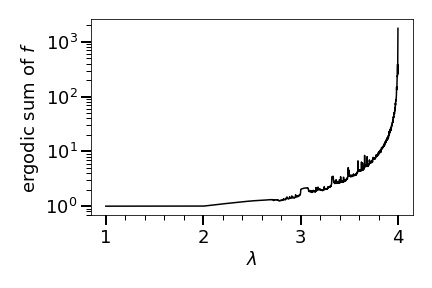
We defer the detailed explanations/comments on Theorem 1.4 to Sections 5 and 6, but to be honest, we found it very surprising that the ergodic sums of change so smooth and stable (except a few bumps) as increases considering the fact (as can be seen from the bifurcation diagram of , Figure 13) that as increases go through a quite a bit of qualitative changes from a stable fixed point, attracting periodic orbit of different periods, and finally chaotic behaviours.
Here is the structure of the rest of the paper. In Section 2, we give necessary definitions involving chaos and explain how we got our first main theorem (Theorem 1.2) together with its (mathematical/economic) interpretations. Next, in Section 3, we give the proofs of Theorem 1.2 and Proposition 1.1. In Section 4, after giving a quick overview of ergodic theory, we explain a generic method to obtain our second main result (Theorem 1.4) with its important stepping stone (Theorem 5.11). Our argument here is a delicate combinations of results from ergodic theory and numerical computations. In Section 5, we give some (mathematical) interpretations of Theorem 1.4 including its connection to a deep result in ergodic theory (Proposition 6.3) of Avila et.al.
All programming files used for numerical calculations and for generating plots in this paper (Jupyter notebooks) are available upon request.
2 Odd period cycles
2.1 Definitions involving a chaos
First, we clarify what we mean by a Li-Yorke chaos, a turbulence, and a topological chaos. (There are several definitions of a chaos in the literature.) The following definitions are taken from [Ruette, 2017, Def. 5.1] and [Block and Coppel, 1992, Chap. \@slowromancapii@]. Let be a continuous map of a closed interval into itself:
Definition 2.1.
We say that exhibits a Li-Yorke chaos if there exists an uncountable scrambled set , that is, for any we have
and for and being a periodic point of ,
Definition 2.2.
We call turbulent if there exist three points, , , and in such that and with either or . Moreover, we call (topologically) chaotic if some iterate of is turbulent.
It is known that a map is topologically chaotic if and only if has a periodic point whose period is not a power of , see [Block and Coppel, 1992, Chap. \@slowromancapii@]. This implies that a map is topologically chaotic if and only if the topological entropy of is positive, see [Block and Coppel, 1992, Chap. \@slowromancapviii@]. In the first part of this paper, we focus on a topological chaos (or a positive topological entropy) in the context of price dynamics. See [Ruette, 2017] for more characterisations and (subtle) mutual relations of various kinds of chaos.
2.2 Explanations and Interpretations of Theorem 1.2
Here, we explain a key result to obtain Theorem 1.2. Along the way, we give definitions for all the unexplained notation (such as and ) in Theorem 1.2. First, we recall the following mathematical result characterising the existence of a topological chaos for a unimodal interval map [Deng et al., 2022, Cor. 3]. Theorem 1.2 is a (highly non-trivial as seen in Section 3) consequence (or a special case) of [Deng et al., 2022, Cor. 3]. Let be the set of continuous maps from a closed interval to itself so that an arbitrary element satisfies the following two properties:
-
1.
there exists with the map strictly decreasing on and strictly increasing on .
-
2.
, , and for all .
For , let . Now we are ready to state [Deng et al., 2022, Cor. 3]:
Proposition 2.3.
Let . The map has an odd-period cycle if and only if and and the second iterate is turbulent if and only if and .
We keep the same notation , , , , , and from Equation (1.1). We write for the restriction of to the closed interval . (We will explain the significance of the number and the reason for the choice of in the next section.) Note that in the next section we will show that (so, is a non-degenerate closed interval) and that is a map to .
Now, we give several comments/interpretations on Theorem 1.2. First, in the next section, we will show that the condition in Theorem 1.2 is the weakest condition for to be economically meaningful (to keep ) and also for to be in . As stated in Introduction, the upper bound for is not really interesting and the real meat is in the lower bounds in parts 2,3, and 4.
Second, it is well-know that the vertical stretch the graph of controls the existence of a chaos: if we stretch the graph further, we are likely to obtain a chaos. Now, looking at Equation (1.1), we see that if we make , , small, or large, the ”valley” of the graph of goes deep down. Also, it is clear that a small makes the graph of ”flat”. Our lower bound agrees with these observations: is an increasing function of , , and a decreasing function of . In other words, it is easy to generate a chaos (small gives a chaos) if , , or is small or is large. We give an economic explanation for this. By looking at the form of the excess demand function (or the demand function of each consumer for good , that is, for consumer 1 and for consumer 2 respectively), we see that goes up very sharply (almost irrespective of the parameter values) after gets close to . To generate a chaos, needs to drop sharply afterwords, that is possible (or at least easy) if , , or is small or is large for the following reasons: 1. if or is small, the demand for good is weak (thus drops sharply), 2. if is small, then the demand of consumer 2 for good (that is excessively strong when is close to ) drops sharply (since the budget for consumer 2 is tight), 3. if is large, when is very high, a large excess supply happens.
Third, part 4 of Theorem 1.2 shows that if is sufficiently large, for any initial , our price dynamics eventually trap inside a (Li-Yorke) chaotic region . This is interesting since parts 1, 2, and 3 say nothing about what is going on outside of . This sort of analysis is not done in [Deng et al., 2022].
2.3 Odd period (but no period three) cycles
To end this section, we give an application of Theorem 1.2. By the Sharkovsky order in [Sharkovsky, 1964], we know that if the map has a cycle of period three, then it also has a cycle of any odd order. Thus, it is natural to guess that if is close to the lower bound for in Theorem 1.2 (but still above the lower bound), the map has an odd period cycle but no period three cycle. We give one example where this is actually the case. Using our concrete characterisation of the existence of an odd period cycle, we obtain:
Proposition 2.4.
Let . If , then the map in Equation (1.1) has an odd period cycle but no period three cycle.
Note that in this case, by Theorem 1.2 a necessary and sufficient condition for the existence of an odd period cycle is . (We use this condition in Section 6.) Our numerical computation (see Section 4 for details) shows that Proposition 2.4 is almost an if and only if statement: for , we get a period three cycle. Although many examples of this sort can be obtained by the same method, a complete characterisation for the existence of a period three cycle for a unimodal map is not known. (Thus it is not possible to obtain the precise value where a bifurcation happens.) We leave it for a future work.
3 Proof of Theorem 1.2
In the following proof, most results follow from direct (but a fairly complicated) algebraic calculations. We give some sketches of our manipulations while pointing some important steps out rather than writing all the details. All calculations can be checked by a computer algebra system, say, Magma [Bosma et al., 1997], Python [Rossum and Drake, 2009], etc.
First, for the function in Equation (1.1), we have and for any . So, is strictly convex (unimodal) and takes its minimum at . We sometimes write for to ease the notation. First of all, since we assume that , we must have for any , hence . This gives that .
Next, we want (a restriction of) to be in . Note that any function in must have some in its interior of the domain, say , with strictly decreasing on and strictly increasing on . Since our is unimodal, this forces to be . Moreover needs to satisfy for all . So in particular, we must have . This implies . Note that since (under the condition ), so we have . Now we set and . (Now it is clear that is non-degenerate.)
Lemma 3.1.
If , then .
Proof.
We need to show three things: (1) and . (2) for all . (3) is a map from to itself. We begin with (2). Let . Then we have . Since and , it is enough to show that . Now , so is equivalent to , that is certainly true (since this is our assumption). Now we show that the same argument gives in (1). (This strict inequality is stronger than we need here, but we need it to prove part 4 of Theorem 1.2, see the proof of Lemma 3.6 below.) We have . Since and , it is enough to show that . We have already shown that this is true. Next we show that . By a direct calculation, we have that is equivalent to . Now the assumption forces .
To prove (3), we need to show that the maximum value of does not exceed (that the minimum value of , that is , is in is clear). Since is unimodal, the maximum of on is taken either at or at . For the first case, we have . For the second case, we need , but this is true by part (1) above.
∎
We have proved part 1 of Theorem 1.2. We assume for the rest of this section (actually for the rest of the paper). Now we are ready to prove parts 2 and 3 of the theorem. In view of Proposition 2.3 and Lemma 3.1, we only need to translate two conditions and (or ) in terms of , , , , and . First we show that
Lemma 3.2.
if and only if .
Proof.
Under the condition , a direct computation shows that is equivalent to . Now the statement follows. ∎
Next we show that
Lemma 3.3.
If , then the set is a singleton, namely (the unique fixed point for ).
Proof.
First, we compute the fixed points of . Solving for , we obtain . So, has the unique fixed point, which we name . It is clear that (this follows from ) and (since is the minimum of ). So, we have . Next, we compute the period points for on . Solving for (with Python), we get . The first is (the fixed point), and the other two points are the period points. We name the last two points as and respectively (). If we show that , we are done. A direct calculation (with Python) shows that is equivalent to (this is our assumption). ∎
Now we assume . (So is a singleton.) Finally we show
Lemma 3.4.
if and only if .
Proof.
This calculation is a bit involved, so we give some details. Let be the fixed point of . Since we know that , we have
We consider the first term of the last expression. A direct calculation shows that if and only if (which we already assumed). So, we have . (The last inequality followed from Lemma 3.2.) Next, a direct calculation shows that the second term of the last expression is positive if and only if . Now we see that under the condition , this is equivalent to . ∎
It is clear that . So by the same argument, we obtain
Lemma 3.5.
if and only if .
Note that . By Proposition 2.3 and Lemmas 3.1, 3.2, 3.3, 3.4, 3.5, we have proved parts 2 and 3 of Theorem 1.2. Finally, we are left to show (part 4 of Theorem 1.2):
Lemma 3.6.
If , then the closed interval is attracting for , that is, for some .
Proof.
Since , we need to prove: (1) if , then for some , (2) if , then for some . Note that if (the first case), then since is a global minimum for , thus we just need to consider the second case. Let . Then we have . (The last strict inequality follows from , see the proof of Lemma 3.1) This shows that if , in each iteration of , the value of drops by at least. So, to prove that is attracted to , it is enough to show that the size of the drop is not too big (thus does not jump over ). Therefore, it is sufficient to have . Since this is equivalent to and under our assumption on , it suffices to show that . After some computations, we obtain
We check that in the last expression, the denominator is strictly positive if (this follows from our assumption). Also, we see that the numerator is positive if .
∎
4 Proofs of Propositions 1.1 and 2.4
Proof of Proposition 1.1.
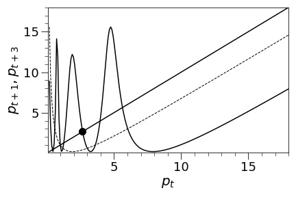
The first part (this paragraph) of the following argument is a replicate of [Bhattacharya and Majumdar, 2007, Proof of Prop. 9.10]. We include this to make the paper self-contained. Let , , and . Then we have , , . So, by the Li-Yorke theorem, there exists a period three cycle. Also, by [Bhattacharya and Majumdar, 2007, Prop. 9.10 and its proof], we know that the choices of and are robust (for this fixed ), so it is clear that there exist open sets and as in Proposition 1.1. Thus, the only thing we need to show is that the choice of is also robust. This follows from the following numerical/graphical argument.
In Figure 2, we plot the graphs of (dashed curve) and (solid curve) together with the line. We see that the solid curve crosses the line at (the big dot) between and . A numerical computation gives , and it is clear that is a point of period three. (From the picture we see that is not a fixed point.) Since the solid curve crosses (but not touching) the line at and is continuous in and , a small perturbation of and does not affect the existence of a period three cycle. So, there exists an open set as required. (Actually, this graphical argument gives the existence of open sets and as well.) ∎
Proof of Proposition 2.4.
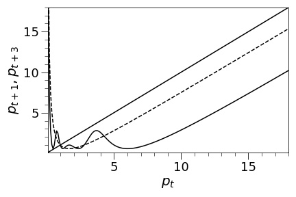
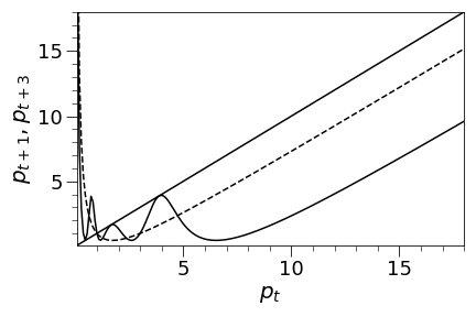
Let , , and . Then by Theorem 1.2 it is clear that the map has an odd period cycle. Only thing we need to show now is that does not have a period three cycle. We use a graphical/numerical argument. In Figures 3, 4, and 5 we plot the graphs of (dashed curve) and (solid curve) with the line. A general pattern is that if we increase , the graph of gets slightly deeper down, and becomes more ”wavy”. (Compare Figure 2 () to Figure 3 () for example.) For Figure 3 (), using a numerical computation, we have checked that the solid curve does not touch/cross the line except at (the fixed point of ). Thus, there is no period three cycle in this case. Likewise, for Figure 4 (), there is no period three cycle (although the solid curve seems touching the line but a numerical computation shows that it is not touching). However, if , a numerical computation shows that there exists a period three cycle. In Figure 5, we plotted the case since the case is indistinguishable from the case in picture. It is clear that the solid curve crosses the line near (that is not a fixed point of ).

∎
5 Ergodic properties: an experimental approach
Our (numerical/theoretical) argument in this and the next sections use ergodic theory. Here, we give a quick review of ergodic theory. If the reader is familiar with ergodic theory, skip Subsection 5.1. Our basic references for ergodic theory are classical [Collet and Eckmann, 1980], [Day, 1998], and [W. de Melo, 1993]. Note that our strategy (philosophy) in this and the next sections stems from [Lyubich, 2012] and [Shen and van Strien, 2014] (these are quite readable expository articles on recent developments of unimodal dynamics). We stress that a deep result by Avila et.al. (Proposition 6.3) theoretically supports our argument.
5.1 Background from ergodic theory
Let be a compact interval on . Let denote the Borel -algebra of . Let be a measure on . A measurable map is called ergodic with respect to if whenever for , then either or . We say that a measure is g-invariant if for any . We write for the Lebesgue measure on . A measure is called absolutely continuous with respect to if whenever for then . We write an ”acim” for a measure that is absolutely continuous with respect to and -invariant (if is clear from the context, we just say ”invariant”). Remember that if is an acim then there exists a (-integrable) density function (Radon-Nikodym derivative) with , see [Collet and Eckmann, 1980, \@slowromancap[email protected]]. It is well-known that if is ergodic with respect to an acim , then we can give an estimate of (hence an estimate of ) using some iterates of , see [Day, 1998, 8.5.2 and 8.5.3] (we use this argument below in Theorem 5.11).
Here, we recall (a special case of) the famous Birkhoff’s ergodic theorem [Day, 1998, Thm. 8.2], which states that under certain conditions the time average of is equal to its space average:
Proposition 5.1.
If has an absolutely continuous invariant measure , is ergodic with respect to , and is -integrable, then
| (5.1) |
In particular, Proposition 5.1 says that (if the conditions are met) the time average of converges to a constant (for almost all ), in other words, we can ”predict” the future on average. We call the integral on the right-hand side (or sometimes the sum inside the limit on the left-hand side) of Equation (5.1), that is (or sometimes ), the ergodic sum of (which we are referring to would be clear from the context). In the following, we try to apply Proposition 5.1 to our price dynamics defined by (with the condition to force that and ). In the following, we write for to ease the notation. So we need to show that has an absolutely continuous invariant measure , is ergodic with respect to , and is -integrable. (The last condition is clear since is continuous and bounded on the compact interval .)
5.2 -unimodal maps
In general, it is pretty difficult to prove the existence of an acim for a measurable transformation except for some special cases such as when is ”expansive” or ”iteratively expansive” as studied in a classical paper of Lasota and Yorke [Lasota and Yorke, 1973]. Recall that is called expansive if is piecewise and for -almost all . A typical example of an expansive map is a well-studied ”tent map” [Day, 1998, 8.5.4 and 8.5.5]. Further recall that a slightly more general ”iteratively expansive” map, that is a piecewise map with for some positive integer for -almost all . From [Lasota and Yorke, 1973], we know that a density function with is a fixed point of the Perron-Frobenius operator from the set of measurable function on to itself, and that a uniform expansion of a map helps a lot to make a ”nice” operator. As a result, it is not too hard to prove the existence of an acim in these (iteratively) expansive cases. See [W. de Melo, 1993, Chap. 5], [Shen and van Strien, 2014, Sec. 4], and [Lyubich, 2012] for an overview of this problem and also see [Sato and Yano, 2012] and [Sato and Yano, 2013] for applications of an acim for an iteratively expansive map in economics.
In this paper, our function is not (even iteratively) expansive since it has a critical point . (So this is a hard case.) Thus, to establish the existence of an acim, we need some deep analytical results to investigate the counter play between the contraction of near the critical point and the expansion of at (that is far from ). Now, we restrict the class of functions we consider to so-called -unimodal maps (due to Singer [Singer, 1978]), whose ergodic properties are well studied, see [Collet and Eckmann, 1980, Part \@slowromancapii@], [W. de Melo, 1993, Chap. 5], [Avila and Moreira, 2005], [Avila et al., 2003] for example. (Our function is actually -unimodal as we will show below.) Let be a measurable transformation defined on a compact interval of .
Definition 5.2.
A function is called -unimodal if the following conditions are satisfied:
-
1.
is .
-
2.
is unimodal with the unique critical point in and except when .
-
3.
The Schwarzian derivative of , that is, is negative except at .
Moreover the critical point is called non-flat and of order if there are positive constants , with
Note that a well-known ”logistic map” ( for ) is -unimodal. The first key result in this section is
Proposition 5.3.
If is -unimodal with a non-flat critical point and without an attracting periodic orbit, then is ergodic with respect to any absolutely continuous measure .
Proof.
Let be -unimodal with a non-flat critical point and without an attracting periodic orbit. Suppose that for some . Then we have . From [W. de Melo, 1993, Thm. 1.2] we know that is ergodic with respect to , so we obtain that or . This yields or since is absolutely continuous. ∎
To end this subsection, we prove that
Lemma 5.4.
The function (restricted to ) is -unimodal and the unique critical point of is non-flat and of order .
Proof.
First, we show that is . We have , , and . Since is positive (so it is not zero), it is clear that is . Second, from Section 2, we know that is unimodal and has a unique critical point at in . It is easy to see that except when . Third, we have except when . Finally, we show that the critical point is non-flat of order . It is clear that is strictly concave and monotone increasing on the compact interval . Also note that the righthand derivative of at is . So is bounded below by and is bounded above by . Likewise, we have that is strictly convex and monotone decreasing on . Also, the lefthand derivative of is . Therefore, is bounded below by and is bounded above by . Thus we see that (on ) is bounded below by and is bounded above by . ∎
5.3 Our strategy and the existence of an acim
The second key result in this section is
Proposition 5.5.
[Collet and Eckmann, 1980, Thm. \@slowromancap[email protected]] If is -unimodal, then every stable periodic orbit attracts at least one of , , or (i.e. the endpoints of or the critical point of ).
Proposition 5.5 means that all ”visible” orbits (in numerical experiments) are orbits containing , , or only (in the long run). We consider that only these visible orbits are meaningful in economics (or in real life) since it is widely believed that every economic modelling is some sort of an approximation of real economic activities and contains inevitable errors. We know that there are totally different point of view for economic modellings, but we do not argue here. Here is the third key result for this section:
Proposition 5.6.
[Collet and Eckmann, 1980, Cor. \@slowromancap[email protected]] If is -unimodal, then has at most one stable periodic orbit, plus possibly a stable fixed point. If the critical point is not attracted to a stable periodic orbit, then has no stable periodic orbit.
In this paper, we interpret our numerical calculations based on Propositions 5.5 and 5.6. In particular, we look at the orbit starting from the critical point , that is (we call this orbit the ”critical orbit”). If the critical orbit seems to eventually converge to a periodic orbit, we conclude that we can see the future: the average price in the long run will be the average price in this attracting periodic orbit. Note that in this case, is neither ergodic nor has an acim since most accumulate around this attracting periodic orbit, but we do not care (since we can still predict the future). Otherwise, we compute (or give an estimate for) the following Lyapunov exponent at the critical point since the existence of a positive Lyapunov exponent at the critical point implies that the critical orbit is repelling and also is a strong indication for the existence of a chaos (hence the existence of an acim, see (CE1) in Proposition 5.8 below):
Definition 5.7.
is called the Lyapunov exponent of at (if the limit exists).
If the Lyapunov exponent (at ) is positive, we test one of the following well-known sufficient conditions (within some numerical bound) to confirm the existence of an acim.
Proposition 5.8.
Suppose that is -unimodal, has no attracting periodic orbit, and the critical point is non-flat. Then has a unique acim and is ergodic with respect to if one of the following conditions is satisfied:
-
1.
Collet-Eckmann conditions (together with some regularity conditions) [Collet and Eckmann, 1983, Sec. 1]:
-
2.
Misiurewicz condition [Misiurewicz, 1981, Thms. 6.2 and 6.3]: The -limit set of does not contain , that is,
-
3.
Nowicki-Van Strien summation condition [Nowicki and van Strien, 1991, Main Thm.]: if is the order of , then
If one of the conditions in Proposition 5.8 is satisfied (within some numerical limitation), we conclude that we can predict the future by Proposition 5.1. We must admit that our argument in this section is not rigorous (we hope to make it rigorous in the future), but we believe that we have provided enough (numerical/theoretical) evidence to support it. We stress that it is very hard to prove the existence of an acim for any non-expansive function (even for an -unimodal ) by a rigorous analytic argument. There are only a few known examples of such, see a famous example due to Ulam and Neumann [Ulam and von Neumann, 1947], also see [Misiurewicz, 1981, Sec. 7 Examples] for more examples.
In this paper, we test Condition 3 (SC) in Proposition 5.8 since it is easy to compute (numerically) and covers the most general class of functions, see [Shen and van Strien, 2014, 4.2] for a comparison of these three sufficient conditions for the existence of an acim, also see [W. de Melo, 1993, Chap. \@slowromancapv@, Sec. 4] for more on (SC). We found that (CE2) was hard to compute since the set can be very large for a large . Also, the -limit set of was difficult to compute for us although (MC) is theoretically beautiful. (For a numerical computation, it is not clear where to set the numerical bound to estimate the -limit set.)
Remark 5.9.
Roughly speaking, all three condtions (CE1), (MC), and (SC) are basically testing the same thing: they (more or less) guarantee that the critical orbit does not accumulate around the critical point . (So, on the critical orbit, the expansion far from the critical point wins against the contraction near the critical point.)
5.4 case
For the rest of the paper, to simplify the exposition and to obtain sharp numerical results, we fix , . Also, in this subsection, we fix (in the next subsection, we let vary). Then we have . In this case, the dynamics exhibit a Li-Yorke chaos as shown in the previous sections. It is easy to see that a similar analysis (as follows) can be done for any .
Here is our main result in this section. (We can predict the future even if is chaotic.)
Theorem 5.10.
There exists an acim (whose estimate is as in Figure 9) for on . Moreover, we have for -almost all .
A few comments are in order. Although we give an estimate of in Figure 9, it is hard to give an explicit formula for (thus it is hard to express in a concrete way). Also, looking at Figure 9 (and its numerical data), we see that the density of is positive in and is zero in . Thus, without a loss, if one wishes, Theorem 5.10 can be stated (in a more readable form) as follows:
Theorem 5.11.
for -almost all .
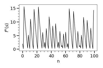
Now we start looking at the model closely. First, following our strategy as in the last subsection, we consider the critical orbit of . Note that the critical point of is . Using the first iterates of , we obtain Figure 6 that shows a chaotic behaviour of the iterates of .
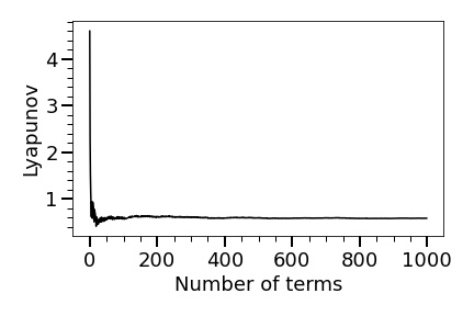
In particular, it seems that has no attracting periodic orbit. To convince the reader that this really the case, we give an estimate for the Lyapunov exponent (using the first 10000 terms of ). Figure 7 shows that the first 1000 terms are enough to estimate the Lyapunov exponent (but we used the first 10000 terms to be safe). We obtain
Lemma 5.12.
.
Remark 5.13.
Let . Note that to compute the Lyapunov exponent we have used the chain rule, that is, (so it is not hard to compute).
Now we check the Nowicki-Van Strien summation condition (SC). Figure 8 shows that the sum in (SC) stabilises if we use the first 100 terms. To be safe, we use 1000 terms to estimate the infinite sum in (SC). We obtain
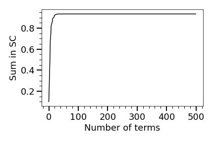
Lemma 5.14.
.
Remark 5.15.
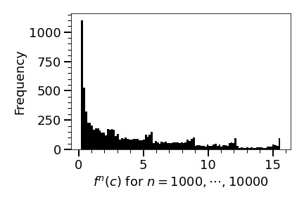
Now we conclude that has a unique acim and is ergodic with respect to by Proposition 5.8. Next, in Figure 9 using with from to (after removing the effect of a transient period) we obatin an estimate of the density function (Radon-Nikodym derivative) with .
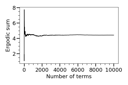
Next, we directly compute the ergodic sum of using the initial and the first terms of . We get
Lemma 5.16.
.
Note that Figure 10 shows that the ergodic sum converges if we use more than terms to estimate it (we use terms to be safe).
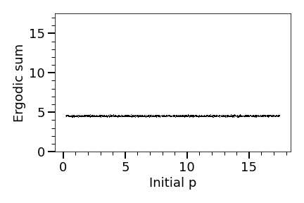
To end this section, we compute the ergodic sums using various initial values. Figure 11 shows the result where the initial is taken from (excluding (the unique fixed point of ). By Figure 11 (where each ergodic sum is estimated using the first terms of ), we conclude that Theorems 5.10 and 5.11 hold and the ergodic sums of converge to somewhere around for (or ) almost all (or ).
6 Ergodic properties: a sensitivity analysis
6.1 Chaos is not too bad
In this final section, we still keep , , but we let vary. Recall that, from Subsection 2.3, we know that there exists an odd period (hence a Li-Yorke chaos) for . We conduct a sensitivity analysis, that is, how the ergodic sums vary when changes with . We know that the unique fixed point of is (independent of ), and the (unique) critical point of is (dependent of ).
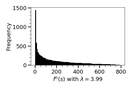
Now, using the same strategy as in the last section, we investigate how the critical orbit behaves for each . Figure 12 is the bifurcation diagram for . We (roughly) see that: (1) for , converges to the unique attracting fixed point (that is ), (2) for , converges to a period- orbit, (3) for (roughly), period doubling bifurcations occur and converges to a period- (8, 16, and so on) orbit, (4) for (possibly starting at around based on results in previous sections), we see a chaos except a few ”windows”, (5) at (or ), we see a period three orbit, (6) for (roughly), again, we see period doubling bifurcations and converges to an orbit of period and so on, (7) for , we see a chaos again except a few windows.
Remark 6.1.
Actually, we have obtained the bifurcation diagram of for , but In Figure 12, we have chopped the diagram at . The reason is that for , the maximum value of grows exponentially, so the diagram gets very skewed (and the part of the diagram shown in Figure 12 becomes almost invisible). For we have obtained a chaotic region (with some windows).
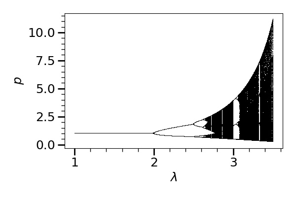
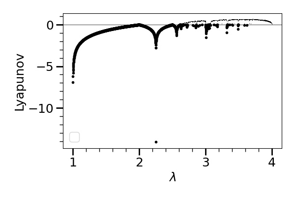
Next, we compute Lyapunov exponents of at for various and obtain Figure 13. We see that roughly speaking the Lyapunov exponent is negative for (thick dots), and positive for (thin dots) except a few ”windows” corresponding to the windows in the bifurcation diagram (Figure 12).
Now, we test (SC) for (we do not care for since it is a non-chaotic region and easy to predict the future). We obtain Figure 14.
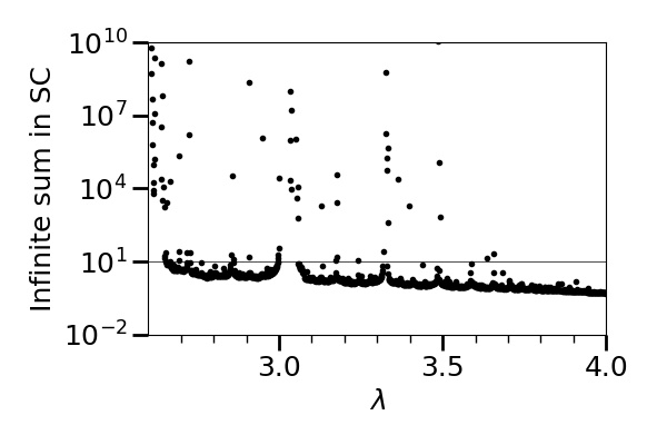
Our argument is based on a numerical computation using terms to estimate the infinite sum in (SC), so we need to decide when we conclude that the infinite sum is finite. We draw the (ad hoc) line at (that is the horizontal line in Figure 14). Basically, we only avoid where (the estimate of) the infinite sum grows exponentially. We hope to rigorously prove that the infinite sums here are finite in the future work.
Here are main results in this section.
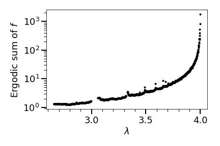
Theorem 6.2.
For values as in Theorem 6.2 (satisfying the SC), we obtain a pretty smooth relation between and the ergodic sums of as in Figure 15 (using terms to estimate the ergodic sums). Extending Theorem 6.2 (and Figure 15) using the naive estimates of the ergodic sum (that is ) for that does not satisfy (SC), we obtain Theorem 1.4 (and Figure 16).
6.2 Comments and interpretations on Theorem 1.4
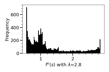
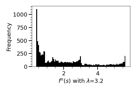
Here, we add a few comments and interpretations on Theorem 1.4: (1) We found it surprising that the overall behaviour of the ergodic sums of is quite smooth and stable considering the fact that as increases go through a quite a bit of qualitative changes from a stable fixed point, attracting periodic orbit of different periods, and finally chaotic behaviours. (2) The gradual increase of the ergodic sum of as increases was unexpected (for us). We knew that as increases, takes more extreme values (very high/very low), but knew nothing about their distributions. To give some (mathematical) explanation for the behaviour (2), we obtained the estimates of distributions of for various using terms in Figures 16, 17, and 18 (see Figure 9 also).
Our computation shows that: (1) The ”shapes” of the distributions of for various look similar: the density is high for a low range and low for a high range. (2) takes more extreme values as becomes large, however, the extension of the upper bound is much greater than that of the lower bound (meaning that for , as becomes large, gets smaller a little bit, but gets larger quite a bit), as shown in Figures 16,17,18, and 9, (3) The distribution gets smoother as becomes large.
We conclude that the gradual increase of the ergodic sum of happens as increases because: (1) takes more extreme values with a great extension of the upper bound (and with a little extension of the lower bound) as increases, (2) The shapes of the distributions do not change much as increases (although it gets smoother), (3) Thus, the average of goes up as increases. We do not know why the overall behaviour of ergodic sums of is so smooth and stable. Also, we do not know why the density curve gets smoother as increases. We leave these issues for a future work.
Theorem 1.4 (and the whole results in this paper) says that a naive estimate of the ergodic sums of (estimate of the future) using a reasonably large number of terms (say terms) is not too bad. To end the paper, we quote a deep result of Avila (2014 fields medalist) and others [Avila et al., 2003, Sec. 3.1, Theorem B] that supports Theorem 1.4.
Proposition 6.3.
In any non-trivial real analytic family of quasiquadratic maps (that contains -unimodal maps), (Lebesgue) almost any map is either regular (i.e., it has an attracting cycle) or stochastic (i.e., it has an acim).
Remark 6.4.
A technical note: ”non-triviality” is guaranteed for our set of maps (parametrised by ) since there exist two maps in this set that are not topologically conjugate. For example, take with (non-chaotic) and with (chaotic). See [Avila et al., 2003, Sec. 2.8, Sec. 2.13, Sec. 3.1] for the precise definitions of ”non-trivial” and ”quasiquadratic” (those are a bit too technical to state here). Also, see [Avila and Moreira, 2005], and [Lyubich, 2012] for more on this.
Remark 6.5.
We need ”Lebesgue almost” (or ”except a set of measure zero”) in Theorems 1.4, 6.2, and Proposition 6.3 since the following (anomalous) examples are known, see [Hofbauer and Keller, 1990] and [Johnson, 1987]: for a quadratic map (parametrised by ), there exists such that does not have an attracting periodic orbit and shows a chaotic behaviour, but does not have an acim. We expect that for our , we obtain examples of the same properties (although we have not checked yet). The point is that we do not care such anomalous cases since the values corresponding to such examples are of Lebesgue measure zero and our approach in this (and the last) section is probabilistic.
Acknowledgements
This research was supported by a JSPS grant-in-aid for early-career scientists (22K13904) and an Alexander von Humboldt Japan-Germany joint research fellowship.
References
- [Avila et al., 2003] Avila, A., Lyubich, M., and de Melo, W. (2003). Regular or stochastic dynamics in real analytic families of unimodal maps. Invent. Math., 154:451–550.
- [Avila and Moreira, 2005] Avila, A. and Moreira, C. (2005). Statistical properties of unimodal maps: the quadratic family. Ann. Math., 161:831–881.
- [Benhabib and Day, 1980] Benhabib, J. and Day, R. (1980). Erratic accumulation. Econ. Lett., 6:113–117.
- [Benhabib and Day, 1982] Benhabib, J. and Day, R. (1982). A characterization of erratic dynamics in the overlapping generations model. J. Econ. Dyn. Control, 4:37–55.
- [Bhattacharya and Majumdar, 2007] Bhattacharya, R. and Majumdar, M. (2007). Random Dynamical Systems. Cambridge University Press.
- [Block and Coppel, 1992] Block, L. and Coppel, W. (1992). Dynamics in One Dimension. Springer, Berlin.
- [Bosma et al., 1997] Bosma, W., Cannon, J., and Playoust, C. (1997). The Magma algebra system \@slowromancapi@: The user language. J. Symb. Comp, 24:235–265.
- [Collet and Eckmann, 1980] Collet, P. and Eckmann, J.-P. (1980). Iterated Maps on the Interval as Dynamical Systems. Birkhäuser, Progress in Mathematics.
- [Collet and Eckmann, 1983] Collet, P. and Eckmann, J.-P. (1983). Positive liapunov exponents and absolute continuity for maps of the interval. Ergodic Theory Dyn. Syst., 3:13–46.
- [Day, 1998] Day, R. (1998). Complex Economic Dynamics, Volume 1: An Introduction to Dynamical Systems and Market Mechanisms. The MIT Press.
- [Day and Shafer, 1985] Day, R. and Shafer, W. (1985). Keynesian chaos. J. Macroecon., 7:277–295.
- [Deng et al., 2022] Deng, L., Khan, M., and Mitra, T. (2022). Continuous unimodal maps in economic dynamics: On easily verifiable conditions for topological chaos. J. Econ. Theory, 201. Article 105446.
- [Hofbauer and Keller, 1990] Hofbauer, F. and Keller, G. (1990). Quadratic maps without asymptotic measure. Comm. Math. Phis, 127:319–337.
- [Johnson, 1987] Johnson, S. (1987). Singular measures without restrictive intervals. Comm. Math. Phys, 110:185–190.
- [Lasota and Yorke, 1973] Lasota, A. and Yorke, J. (1973). On the existence of invariant measures for piecewise monotonic transformations. Trans. Amer. Math. Soc., 186:481–488.
- [Li and Yorke, 1975] Li, T. and Yorke, J. (1975). Period three implies chaos. Amer. Math. Monthly, 82:985–992.
- [Lyubich, 2012] Lyubich, M. (2012). Forty years of unimodal dynamics: on the occasion of artur avila winning the brin prize. J. Mod. Dyn., 6:183–203.
- [Misiurewicz, 1981] Misiurewicz, M. (1981). Absolutely continuous measures for certain maps of an interval. IHÉS Publ. Math., 53:17–51.
- [Nishimura and Yano, 1996] Nishimura, K. and Yano, M. (1996). Chaotic solutions in dynamic linear programming. Chaos Solitons Fractals, 7:1941–1953.
- [Nowicki and van Strien, 1991] Nowicki, T. and van Strien, S. (1991). Invariant measures exist under a summability condition for unimodal maps. Invent. Math., 105:123–136.
- [Rossum and Drake, 2009] Rossum, G. and Drake, F. (2009). Python 3 Reference Manual. CreateSpace, Scotts Valley, CA.
- [Ruette, 2017] Ruette, S. (2017). Chaos on the Interval. American Mathematical Society, Providence.
- [Sato and Yano, 2012] Sato, K. and Yano, M. (2012). A simple condition for uniqueness of the absolutely continuous ergodic measure and its application to economic models. AIP Conf. Proc., 1479:737–740.
- [Sato and Yano, 2013] Sato, K. and Yano, M. (2013). Ergodic chaos for non-expansive economic models. Int. J. Econ. Theory, 9:57–67.
- [Sharkovsky, 1964] Sharkovsky, A. (1964). Co-existence of cycles of a continuous mapping of the line into itself. Ukr. Math. J., 16:61–71.
- [Shen and van Strien, 2014] Shen, W. and van Strien, S. (2014). Recent developments in interval dynamics. Proc. Int. Cong. Math., 3:699–719.
- [Singer, 1978] Singer, D. (1978). Stable orbits and bifurcations of maps of the interval. SIAM J. Appl. Math, 35:260–267.
- [Ulam and von Neumann, 1947] Ulam, S. and von Neumann, J. (1947). On combinations of stochastic and deterministic processes. Bull. Amer. Math. Soc., 53:1120.
- [W. de Melo, 1993] W. de Melo, S. v. S. (1993). One-Dimensional Dynamics. Springer.