Odd-parity topological superconductivity in kagome metal RbV3Sb5
Abstract
Kagome superconductors AV3Sb5 (A=K, Rb, Cs) have sparked considerable interest due to the presence of several intertwined symmetry-breaking phases within a single material. Recently, hysteresis and reentrant superconductivity were observed experimentally through magnetoresistance measurements in RbV3Sb5 [Ref. [1]], providing strong evidence of a spontaneous time-reversal symmetry breaking superconducting state. The unconventional magnetic responses, combined with crystalline symmetry, impose strong constraints on the possible pairing symmetries of the superconducting state. In this work, we propose that RbV3Sb5 is an odd-parity superconductor characterized by spin-polarized Cooper pairs. The hysteresis in magnetoresistance and the reentrant superconductivity can both be explained by the formation and evolution of superconducting domains composed of non-unitary pairing. Considering the nodal properties of the kagome superconductor RbV3Sb5, it is topological and characterized by Majorana zero modes at its boundary, which can be detected through tunneling experiments.
Introduction.—The quasi-2D kagome superconductors AV3Sb5 (A=K, Rb, Cs) are widely studied due to the presence of many intriguing phases in it [2, 3, 4, 5, 6], such as time-reversal-symmetry-breaking (TRSB) charge density wave [7, 8, 9, 10, 11, 12, 13, 14, 15], charge bond orders [16, 17, 18], nematic phase [19, 20, 21, 22, 23], superconductivity [24, 25, 26, 27, 28, 29, 30, 31, 32] and pair density wave [33, 34, 35, 36]. Interestingly, the in-plane magnetic response of superconductivity in RbV3Sb5 has recently been found to be highly non-trivial, as reported in Ref. [1]. In this experiment, the in-plane upper critical field exhibits anisotropy and demonstrates a two-fold symmetry. Additionally, hysteresis in resistance and the reentrance of superconductivity are observed under an in-plane magnetic field. These findings impose strong constraints on the pairing symmetry and rule out the conventional superconductivity in RbV3Sb5, necessitating a new theory to elucidate the superconductivity in this kagome superconductor.
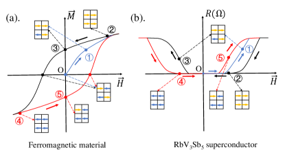
The hysteresis of resistance observed in RbV3Sb5 indicates the breaking of time-reversal symmetry in the superconducting state [1]. This type of superconductivity is characterized by odd-parity and spin-polarized Cooper pairs (i.e. nonunitary). By taking into account the spin polarization of the superconducting states, the hysteresis can be explained using a domain picture. As illustrated in Fig. 1, the superconducting domains with spin-polarization resemble ferromagnetic domains. In this context, the superconducting domains with spin-polarization along the positive and negative directions are referred to as positive and negative domains, respectively. Switching the direction of the magnetic field induces a metastable state that contains two types of domains with opposite spin polarization, as shown at step \small{3}⃝ in Fig. 1 (b). Compared with the superconducting state at step \small{4}⃝ which only contains negative domains, the metastable state at step \small{3}⃝ exhibits higher energy and a lower transition temperature when the magnetic field is along the negative direction. Therefore, the hysteresis is observed during the field-sweeping process (\small{2}⃝ \small{3}⃝ \small{4}⃝ \small{5}⃝). More importantly, the existence of the metastable state is strongly supported by the current quenching experiment. Initially, a large current can be applied to fully suppress the metastable state with finite resistance at step \small{3}⃝. After removing the current, due to the presence of a magnetic field along the negative direction, the system transitions into the superconducting state with only negative domains, which exhibit zero resistance, as shown at step \small{4}⃝.
Moreover, the reentrance of the superconductivity observed in the experiment at around 400 mK can also be understood by the domain picture. When the magnetic field changes sign from negative to positive, the negative domains become less energetically favorable. Due to thermal effects near the superconducting transition temperature, these negative domains shrink and become disconnected, resulting in a finite-resistance state. As the magnetic field continues to increase in the positive direction, the positive domains become energetically favorable, grow larger, and connect with each other, leading to the reappearance of a zero-resistance state.
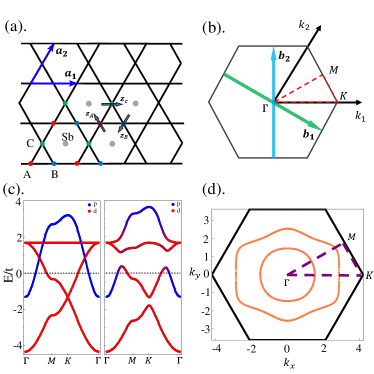
The minimal model for the normal state of kagome superconductor.—First of all, we construct a four-orbital (eight-band) minimal model to describe the normal state of the kagome superconductor RbV3Sb5. As discussed in the previous work [37], the -orbitals of V atoms and the -orbitals of the in-plane Sb atoms have different parities, leading to the spin-orbital-parity coupling (SOPC) terms between them [38, 39]. Fig. 2 (a) shows the real space structure of the kagome plane in RbV3Sb5, and the Brillouin zone of the kagome structure is shown in Fig. 2 (b).
The corresponding Hamiltonian can be expressed as:
| (1) |
where the specific form of can be found in Supplemental Material [40]. The basis of the Hamiltonian is . In the normal state, the band structures without and with SOPC along the high-symmetry line are shown on the left and right sides of Fig. 2 (c), respectively.
The construction of pseudospin basis.—In the presence of SOPC, spin is no longer a good quantum number. However, due to the presence of inversion and time-reversal symmetry, the bands of the 4-orbital minimal model remain doubly degenerate at every point. Therefore, we can define a pseudospin basis in which the pseudospin transforms identically to the real spin (or magnetic moment) under symmetry operations. This pseudospin basis is referred to as manifestly covariant Bloch basis (MCBB) [41, 42, 43, 39, 38, 44]. To construct the MCBB, we project the four-orbital (eight-band) model onto the band basis and select two degenerate bands near the Fermi energy as target bands. Then the pseudospin operators are derived by applying the projector onto the spin operators in the real spin basis. Subsequently, we can expand these pseudospin operators using linear combinations of the Pauli matrices (Further details can be found in the Supplemental Material [40]).
When applying a magnetic field , the effective two-band Hamiltonian can be written as:
| (2) |
where arises from the expansion of pseudospin operators using Pauli matrices. In the Eq. (2), we define an effective magnetic field: , which acts on the pseudospin space. represents the dispersion of the band near the Fermi surface.
The pairing symmetry and superconducting order parameter—Considering the nematic normal state [19], the point group describing the symmetry of normal states in the kagome superconductor becomes . Under MCBB, since we focus on the pseudospin triplet pairing states, only the irreducible representations (irreps) with odd parity are considered. The corresponding order parameters in these channels are listed in Table 5.
| Representations | order parameter |
|---|---|
| ; . | |
| ; . | |
It can be concluded that if the superconducting state belongs to a single irreducible representation (irrep), this superconducting state cannot be nonunitary and, therefore, is not consistent with the aforementioned mechanism for the observed hysteresis and reentrance in superconducting states. Thus, a natural consideration to construct the nonunitary paring is to combine different irreps, by assuming they have similar critical temperatures. This approach is an analog to the theoretical framework proposed for the heavy fermion superconductor [45, 46, 47, 48]. By considering the nodal properties of the superconducting states [49], we choose, without loss of generality, the order parameters with point nodes located along the axis. The nonunitary order parameter with an in-plane magnetic moment can generally be written as:
| (3) |
where the parameter controls the direction of the spin polarization of the Cooper pairs in MCBB. For example, the order parameter represents a nodal superconducting state with spin polarization along the -direction, corresponding to . The parameter controls the amplitude of the Cooper pair’s spin polarization, labeled by , with ranging from to . For or , the amplitude of the Cooper pair’s spin-polarization is zero, resulting in a unitary superconducting state. In contrast, for , the superconducting state is non-unitary and fully polarized, with half of the electrons remaining unpaired.
In our consideration, both of the two Fermi surfaces composed of the and orbitals (annular Fermi surfaces as shown in Fig.2 (d)) take part in the superconducting state. The order parameter given in Eq. (3) naturally gives rise to different gap amplitudes for the inner and outer Fermi surfaces, then the superconducting states are expected to exhibit a two-gap behavior. This is consistent with experimental observations of multi-gap signatures in kagome superconductors [49, 50].
The upper critical field of the superconductivity in monolayer limit.—In this section, within the MCBB, we calculate the upper critical field of the superconductivity in monolayer limit by using the gap equation. From the linearized Eliashberg equation, the gap equation of superconductivity can be derived as [51, 52]:
| (4) | ||||
where the is the Matsubara Greens function constructed by the effective two-band Hamiltonian in Eq. (2).
We simplify the gap equation by using the decoupling of the interaction [52]:
| (5) |
The decoupling constant is represented by , which is proportional to the strength of the interaction.
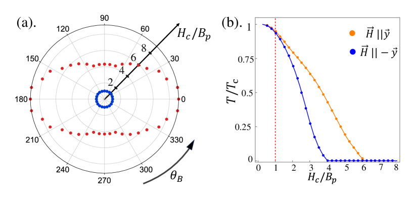
Furthermore, in the experiment [1], the hysteresis behavior remains unchanged even when the initial superconducting state is established through the zero-field cooling process. This fact confirms the intrinsic unbalance between the amplitudes of two equal spin pairing states with opposite spin-polarization. Therefore, we can assume the intrinsic polarization or is selected by the form of the decoupling constant . With this assumption, we can numerically solve the gap equation, accounting for the presence of the nematic normal state. In Fig. 3 (a), a two-fold symmetric upper critical field is shown. During this calculation, the direction of the magnetic moment for the superconducting order parameter is chosen to align with the applied magnetic field, minimizing the total energy of this superconductor. However, during the field-sweeping process, when the magnetic field changes sign, the superconductor enters into a metastable state which is formed by two superconducting domains with opposite magnetic moments. Thus, we also calculate the upper critical field for superconducting states with magnetic moments opposite to the applied magnetic field. Compared to the superconducting states where the magnetic moments align with the applied magnetic field, those with opposite magnetic moments have higher energy and a lower upper critical field, as shown in Fig. 3 (b).
Although the calculated upper critical fields in the monolayer limit exceed the Pauli limit, experiments show that the upper critical field of kagome RbV3Sb5 does not exceed this limit. This discrepancy is attributed to the suppression of the upper critical field induced by interlayer coupling [53, 54, 55]. The violation of the Pauli limit observed in another kagome superconductor, CsSb5 [50], which exhibits much weaker interlayer coupling [27], further supports this mechanism.
Topological properties.—In the previous section, we introduced the superconducting order parameter and discussed the superconducting properties of the kagome material within the MCBB. The results indicate that the superconductivity in this material exhibits point nodes and breaks time-reversal symmetry. Building on these nodal features and the TRSB behavior, in this section, we will explore the topological properties of the superconducting state described by the order parameter in Eq. (3). For convenience, we rewrite the order parameter as , the relation between and , can be obtained by comparing it with Eq. (3). The Bogoliubov-de Gennes (BdG) Hamiltonian of the superconductivity at zero magnetic field case can be expressed as:
| (6) | ||||
where and represent the Pauli matrices in Nambu and pseudospin space, respectively. In , the magnetic field is taken to be . This Hamiltonian can be diagonalized into two decoupled blocks by a unitary matrix (whose specific form can be found in Supplemental Material [40]):
| (7) |
where
| (8) |
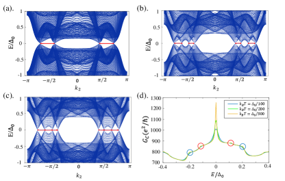
In the normal state, there are two annular Fermi surfaces around the point of the Brillouin zone. Additionally, the zeros of the order parameter are located along the axis. As a result, the superconductivity described by exhibits four point nodes. In Fig. 4(a), the open boundary calculation at zero filed case shows the presence of Majorana zero modes (so-called edge Majorana flat band, EMFB) [56, 57, 58, 59, 60, 61, 62, 63, 64, 65, 66] between two point nodes belonging to different Fermi surfaces. The -coordinates of the four point nodes are , , and , respectively, where the latter subscript in momentum represents different Fermi surfaces ( represents outer Fermi surface, and represents inner Fermi surface). The winding numbers for the blocks of the Hamiltonian and are labeled as and , respectively. We calculate these winding numbers at some representative under two different conditions: and . The results are presented in Table. 2.
Because two blocks of the Hamiltonian do not couple to each other, the EMFBs are robust in zero-field cases. Both two blocks of the Hamiltonian preserve the ”effective time-reversal-symmetry” (, ) and the particle-hole symmetry (), indicating that both blocks belong to class [67, 68, 57, 62, 69, 70, 71].
The two blocks of the Hamiltonian couple to each other when a magnetic field is applied in an in-plane direction. Without considering the momentum dependence of the effective magnetic field , the Hamiltonian for a magnetic field applied along the -axis can be expressed as: , where . We then perform the open boundary calculation under two different conditions: and . The results are shown in Fig. 4 (b) and (c), respectively. The evolution of the EMFB under a magnetic field differs between these two conditions. However, in both cases, the open boundary spectrum reveals the existence of a single EMFB. The winding numbers of both cases at some representative can also be calculated, and the results are shown in Table. 3.
When considering the momentum dependence of the effective magnetic field, although obtaining the open boundary spectrum is difficult, we can still calculate the winding number of the Hamiltonian. The results are the same as those presented in Table 3, indicating that the properties of the EMFB remain unchanged compared to the case where the momentum dependence of the effective magnetic field is not considered. Details of the open boundary spectrum and the winding number calculation in this section can be found in the Supplemental Material [40].
Tunneling properties.—In this section, we propose a tunnel-junction experiment to detect the nodal topological superconductivity in kagome superconductor RbV3Sb5. At zero-field case, we calculate the tunneling spectra of the model in Eq. (6) using the recursive Green’s function method [72, 73, 74, 75] (The details for the calculation can be found in Supplemental Material [40]). As shown in Fig. 4(d), due to the existence of the EMFB, a zero-bias conductance peak emerges as the consequence of the resonant Andreev reflection processes [76, 77], which can be evidence for the nodal topological superconductivity. Additionally, apart from the zero-bias peak, the tunneling conductance also exhibits additional peaks around and , as shown in Fig. 4 (d). These additional peaks are attributed to the multigap behavior of the quasiparticle bands in the superconducting state, arising from the different gap amplitudes on the two annular Fermi surfaces (details can be found in the Supplemental Material [40]).
Conclusion and discussion.—In conclusion, RbV3Sb5 is an odd parity superconductor with non-trivial topological properties. The observed hysteresis in resistance and reentrance of superconductivity are attributed to the spin-triplet pairing components with finite spin-polarization. This type of spin-triplet pairing breaks time-reversal symmetry, leading to the formation of two types of superconducting domains with opposite spin-polarization. The formation and evolution of these two types of superconducting domains under an in-plane magnetic field can account for the hysteresis in magnetoresistance and the reentrant superconductivity observed in the experiment.
Within a pseudo-spin basis, we investigate the topological properties of this kagome superconductor. The open boundary spectrum reveals the presence of Majorana flat bands localized at the boundary of the superconductor. This suggests that a large local density of states can be observed at the boundary through tunneling experiments. Additionally, by combining the superconducting order parameter with the two annular Fermi surfaces in the normal state, we anticipate observing a two-gap behavior in this kagome superconductor, consistent with experimental observations [49]. This kind of two-gap behavior can also lead to additional peaks in the tunneling conductance, which could help identify the superconducting order parameters when the Fermi surfaces of the normal state are known. Interestingly, when considering the repulsive interaction, the two annular Fermi surfaces naturally favor -wave superconductivity within the framework of the Kohn-Luttinger mechanism [78, 79, 80, 81, 82, 83], potentially explaining the origin of the odd-parity superconductivity observed in kagome RbV3Sb5. This will be further explored in our future work.
Acknowledgements—K. T. L. acknowledges the support of the Ministry of Science and Technology, China, and Hong Kong Research Grant Council through Grants No. 2020YFA0309600, No. RFS2021-6S03, No. C6025-19G, No. AoE/P-701/20, No. 16310520, No. 16307622, and No. 16309223.
References
- Wang et al. [2024] S. Wang, X. Feng, J.-Z. Fang, J.-P. Peng, Z.-T. Sun, J.-J. Yang, J. Liu, J.-J. Zhao, J.-K. Wang, X.-J. Liu, Z.-N. Wu, S. Sun, N. Kang, X.-S. Wu, Z. Zhang, X. Fu, K. T. Law, B.-C. Lin, and D. Yu, Spin-polarized p-wave superconductivity in the kagome material RbV3Sb5 (2024), arXiv:2405.12592 [cond-mat.str-el] .
- Ortiz et al. [2019] B. R. Ortiz, L. C. Gomes, J. R. Morey, M. Winiarski, M. Bordelon, J. S. Mangum, I. W. Oswald, J. A. Rodriguez-Rivera, J. R. Neilson, S. D. Wilson, et al., Physical Review Materials 3, 094407 (2019).
- Ortiz et al. [2020] B. R. Ortiz, S. M. Teicher, Y. Hu, J. L. Zuo, P. M. Sarte, E. C. Schueller, A. M. Abeykoon, M. J. Krogstad, S. Rosenkranz, R. Osborn, et al., Physical Review Letters 125, 247002 (2020).
- Yin et al. [2022] J.-X. Yin, B. Lian, and M. Z. Hasan, Nature 612, 647 (2022).
- Wang et al. [2023a] Y. Wang, H. Wu, G. T. McCandless, J. Y. Chan, and M. N. Ali, Nat Rev Phys 5, 635–658 (2023a).
- Guguchia et al. [2023a] Z. Guguchia, R. Khasanov, and H. Luetkens, npj Quantum Materials 8, 41 (2023a).
- Jiang et al. [2021] Y.-X. Jiang, J.-X. Yin, M. M. Denner, N. Shumiya, B. R. Ortiz, G. Xu, Z. Guguchia, J. He, M. S. Hossain, X. Liu, et al., Nature materials 20, 1353 (2021).
- Yu et al. [2021a] L. Yu, C. Wang, Y. Zhang, M. Sander, S. Ni, Z. Lu, S. Ma, Z. Wang, Z. Zhao, H. Chen, et al., arXiv preprint arXiv:2107.10714 (2021a).
- Yang et al. [2020] S.-Y. Yang, Y. Wang, B. R. Ortiz, D. Liu, J. Gayles, E. Derunova, R. Gonzalez-Hernandez, L. Šmejkal, Y. Chen, S. S. Parkin, et al., Science advances 6, eabb6003 (2020).
- Yu et al. [2021b] F. Yu, T. Wu, Z. Wang, B. Lei, W. Zhuo, J. Ying, and X. Chen, Physical Review B 104, L041103 (2021b).
- Feng et al. [2021a] X. Feng, K. Jiang, Z. Wang, and J. Hu, Science bulletin 66, 1384 (2021a).
- Feng et al. [2021b] X. Feng, Y. Zhang, K. Jiang, and J. Hu, Physical Review B 104, 165136 (2021b).
- Lin and Nandkishore [2021] Y.-P. Lin and R. M. Nandkishore, Physical Review B 104, 045122 (2021).
- Denner et al. [2021] M. M. Denner, R. Thomale, and T. Neupert, Physical Review Letters 127, 217601 (2021).
- Christensen et al. [2021] M. H. Christensen, T. Birol, B. M. Andersen, and R. M. Fernandes, Physical Review B 104, 214513 (2021).
- Wagner et al. [2023] G. Wagner, C. Guo, P. J. Moll, T. Neupert, and M. H. Fischer, Physical Review B 108, 125136 (2023).
- Wu et al. [2022] S. Wu, B. R. Ortiz, H. Tan, S. D. Wilson, B. Yan, T. Birol, and G. Blumberg, Physical Review B 105, 155106 (2022).
- Wang et al. [2023b] Y. Wang, T. Wu, Z. Li, K. Jiang, and J. Hu, Physical Review B 107, 184106 (2023b).
- Xu et al. [2022] Y. Xu, Z. Ni, Y. Liu, B. R. Ortiz, Q. Deng, S. D. Wilson, B. Yan, L. Balents, and L. Wu, Nature physics 18, 1470 (2022).
- Li et al. [2022] H. Li, H. Zhao, B. R. Ortiz, T. Park, M. Ye, L. Balents, Z. Wang, S. D. Wilson, and I. Zeljkovic, Nature Physics 18, 265 (2022).
- Grandi et al. [2023] F. Grandi, A. Consiglio, M. A. Sentef, R. Thomale, and D. M. Kennes, Physical Review B 107, 155131 (2023).
- Tazai et al. [2023] R. Tazai, Y. Yamakawa, and H. Kontani, Nature Communications 14, 7845 (2023).
- Jiang et al. [2023] Z. Jiang, H. Ma, W. Xia, Z. Liu, Q. Xiao, Z. Liu, Y. Yang, J. Ding, Z. Huang, J. Liu, et al., Nano Letters 23, 5625 (2023).
- Wu et al. [2021] X. Wu, T. Schwemmer, T. Müller, A. Consiglio, G. Sangiovanni, D. Di Sante, Y. Iqbal, W. Hanke, A. P. Schnyder, M. M. Denner, et al., Physical review letters 127, 177001 (2021).
- Ortiz et al. [2021] B. R. Ortiz, P. M. Sarte, E. M. Kenney, M. J. Graf, S. M. Teicher, R. Seshadri, and S. D. Wilson, Physical Review Materials 5, 034801 (2021).
- Mu et al. [2021] C. Mu, Q. Yin, Z. Tu, C. Gong, H. Lei, Z. Li, and J. Luo, Chinese Physics Letters 38, 077402 (2021).
- Yin et al. [2021] Q. Yin, Z. Tu, C. Gong, Y. Fu, S. Yan, and H. Lei, Chinese Physics Letters 38, 037403 (2021).
- Ni et al. [2021] S. Ni, S. Ma, Y. Zhang, J. Yuan, H. Yang, Z. Lu, N. Wang, J. Sun, Z. Zhao, D. Li, et al., Chinese Physics Letters 38, 057403 (2021).
- Zhao et al. [2021a] H. Zhao, H. Li, B. R. Ortiz, S. M. Teicher, T. Park, M. Ye, Z. Wang, L. Balents, S. D. Wilson, and I. Zeljkovic, Nature 599, 216 (2021a).
- Zhao et al. [2021b] C. Zhao, L. Wang, W. Xia, Q. Yin, J. Ni, Y. Huang, C. Tu, Z. Tao, Z. Tu, C. Gong, et al., arXiv preprint arXiv:2102.08356 (2021b).
- Wang et al. [2021] Q. Wang, P. Kong, W. Shi, C. Pei, C. Wen, L. Gao, Y. Zhao, Q. Yin, Y. Wu, G. Li, et al., Advanced Materials 33, 2102813 (2021).
- Rømer et al. [2022] A. T. Rømer, S. Bhattacharyya, R. Valentí, M. H. Christensen, and B. M. Andersen, Phys. Rev. B 106, 174514 (2022).
- Wu et al. [2023] Y.-M. Wu, P. Nosov, A. A. Patel, and S. Raghu, Physical Review Letters 130, 026001 (2023).
- Jin et al. [2022] J.-T. Jin, K. Jiang, H. Yao, and Y. Zhou, Physical Review Letters 129, 167001 (2022).
- Zhou and Wang [2022] S. Zhou and Z. Wang, Nature Communications 13, 7288 (2022).
- Schwemmer et al. [2023] T. Schwemmer, H. Hohmann, M. Dürrnagel, J. Potten, J. Beyer, S. Rachel, Y.-M. Wu, S. Raghu, T. Müller, W. Hanke, et al., arXiv preprint arXiv:2302.08517 (2023).
- Gu et al. [2022] Y. Gu, Y. Zhang, X. Feng, K. Jiang, and J. Hu, Phys. Rev. B 105, L100502 (2022).
- Xie et al. [2020] Y.-M. Xie, B. T. Zhou, and K. T. Law, Physical Review Letters 125, 107001 (2020).
- Zhang et al. [2023] E. Zhang, Y.-M. Xie, Y. Fang, J. Zhang, X. Xu, Y.-C. Zou, P. Leng, X.-J. Gao, Y. Zhang, L. Ai, et al., Nature Physics 19, 106 (2023).
- [40] The Supplementray material of ”Odd-parity topological superconductivity in kagome metal RbV3Sb5”. Including three parts, I. Model Hamiltonian of RbV3Sb5, II. Linearized gap equation in MCBB representation, III. Topological superconductivity.
- Yip [2013] S.-K. Yip, Phys. Rev. B 87, 104505 (2013).
- Fu [2015] L. Fu, Physical review letters 115, 026401 (2015).
- Yip [2016] S. Yip, arXiv preprint arXiv:1609.04152 (2016).
- Fischer et al. [2023] M. H. Fischer, M. Sigrist, D. F. Agterberg, and Y. Yanase, Annual Review of Condensed Matter Physics 14, 153 (2023).
- Jiao et al. [2020] L. Jiao, S. Howard, S. Ran, Z. Wang, J. O. Rodriguez, M. Sigrist, Z. Wang, N. P. Butch, and V. Madhavan, Nature 579, 523 (2020).
- Hayes et al. [2021] I. M. Hayes, D. S. Wei, T. Metz, J. Zhang, Y. S. Eo, S. Ran, S. R. Saha, J. Collini, N. P. Butch, D. F. Agterberg, et al., Science 373, 797 (2021).
- Aoki et al. [2022] D. Aoki, J.-P. Brison, J. Flouquet, K. Ishida, G. Knebel, Y. Tokunaga, and Y. Yanase, Journal of Physics: Condensed Matter 34, 243002 (2022).
- Ishihara et al. [2023] K. Ishihara, M. Roppongi, M. Kobayashi, K. Imamura, Y. Mizukami, H. Sakai, P. Opletal, Y. Tokiwa, Y. Haga, K. Hashimoto, et al., Nature Communications 14, 2966 (2023).
- Guguchia et al. [2023b] Z. Guguchia, C. Mielke III, D. Das, R. Gupta, J.-X. Yin, H. Liu, Q. Yin, M. H. Christensen, Z. Tu, C. Gong, et al., Nature communications 14, 153 (2023b).
- Hossain et al. [2024] M. S. Hossain, Q. Zhang, E. S. Choi, D. Ratkovski, B. Lüscher, Y. Li, Y.-X. Jiang, M. Litskevich, Z.-J. Cheng, J.-X. Yin, et al., arXiv preprint arXiv:2411.15333 (2024).
- Frigeri et al. [2004] P. Frigeri, D. Agterberg, A. Koga, and M. Sigrist, Physical Review Letters 92, 097001 (2004).
- Sigrist [2009] M. Sigrist, in AIP Conference Proceedings, Vol. 1162 (American Institute of Physics, 2009) pp. 55–96.
- Lawrence and Doniach [1971] W. Lawrence and S. Doniach, in Proceedings of the 12th International Conference on Low Temperature Physics (1971) p. 361.
- Klemm et al. [1975] R. A. Klemm, A. Luther, and M. Beasley, Physical Review B 12, 877 (1975).
- Ruggiero et al. [1980] S. Ruggiero, T. Barbee Jr, and M. Beasley, Physical Review Letters 45, 1299 (1980).
- Sato and Fujimoto [2009] M. Sato and S. Fujimoto, Physical Review B 79, 094504 (2009).
- Hasan and Kane [2010] M. Z. Hasan and C. L. Kane, Reviews of modern physics 82, 3045 (2010).
- Sau et al. [2010] J. D. Sau, R. M. Lutchyn, S. Tewari, and S. D. Sarma, Physical review letters 104, 040502 (2010).
- Alicea [2010] J. Alicea, Physical Review B 81, 125318 (2010).
- Oreg et al. [2010] Y. Oreg, G. Refael, and F. Von Oppen, Physical review letters 105, 177002 (2010).
- Schnyder and Ryu [2011] A. P. Schnyder and S. Ryu, Physical Review B 84, 060504 (2011).
- Qi and Zhang [2011] X.-L. Qi and S.-C. Zhang, Reviews of Modern Physics 83, 1057 (2011).
- Alicea [2012] J. Alicea, Reports on progress in physics 75, 076501 (2012).
- Beenakker [2013] C. Beenakker, Annu. Rev. Condens. Matter Phys. 4, 113 (2013).
- Schnyder and Brydon [2015] A. P. Schnyder and P. M. Brydon, Journal of Physics: Condensed Matter 27, 243201 (2015).
- Zhou et al. [2016] B. T. Zhou, N. F. Yuan, H.-L. Jiang, and K. T. Law, Physical Review B 93, 180501 (2016).
- Zirnbauer [1996] M. R. Zirnbauer, Journal of Mathematical Physics 37, 4986 (1996).
- Altland and Zirnbauer [1997] A. Altland and M. R. Zirnbauer, Physical Review B 55, 1142 (1997).
- Matsuura et al. [2013] S. Matsuura, P.-Y. Chang, A. P. Schnyder, and S. Ryu, New Journal of Physics 15, 065001 (2013).
- Chiu et al. [2016] C.-K. Chiu, J. C. Teo, A. P. Schnyder, and S. Ryu, Reviews of Modern Physics 88, 035005 (2016).
- Sato and Ando [2017] M. Sato and Y. Ando, Reports on Progress in Physics 80, 076501 (2017).
- Fisher and Lee [1981] D. S. Fisher and P. A. Lee, Physical Review B 23, 6851 (1981).
- Lee and Fisher [1981] P. A. Lee and D. S. Fisher, Physical Review Letters 47, 882 (1981).
- Sun and Xie [2009] Q.-f. Sun and X. Xie, Journal of Physics: Condensed Matter 21, 344204 (2009).
- Liu et al. [2012] J. Liu, A. C. Potter, K. T. Law, and P. A. Lee, Physical review letters 109, 267002 (2012).
- Law et al. [2009] K. T. Law, P. A. Lee, and T. K. Ng, Physical review letters 103, 237001 (2009).
- Wimmer et al. [2011] M. Wimmer, A. Akhmerov, J. Dahlhaus, and C. Beenakker, New Journal of Physics 13, 053016 (2011).
- Kohn and Luttinger [1965] W. Kohn and J. Luttinger, Physical Review Letters 15, 524 (1965).
- Ghazaryan et al. [2021] A. Ghazaryan, T. Holder, M. Serbyn, and E. Berg, Physical review letters 127, 247001 (2021).
- You and Vishwanath [2022] Y.-Z. You and A. Vishwanath, Physical Review B 105, 134524 (2022).
- Qin et al. [2023] W. Qin, C. Huang, T. Wolf, N. Wei, I. Blinov, and A. H. MacDonald, Physical Review Letters 130, 146001 (2023).
- Ghazaryan et al. [2023] A. Ghazaryan, T. Holder, E. Berg, and M. Serbyn, Physical Review B 107, 104502 (2023).
- Kumar et al. [2024] A. Kumar, A. S. Patri, and T. Senthil, arXiv preprint arXiv:2410.09148 (2024).
- Wang et al. [2023c] Y. Wang, H. Wu, G. T. McCandless, J. Y. Chan, and M. N. Ali, Nature Reviews Physics 5, 635–658 (2023c).
- Wilson and Ortiz [2023] S. D. Wilson and B. R. Ortiz, arXiv preprint arXiv:2311.05946 (2023).
SUPPLEMENTARY NOTE 1: MODEL HAMILTONIAN OF RbV3Sb5
.1 Lattice model with spin-orbit-parity coupling and nematicity
, ,
| (9) |
| (10) |
where , , , , shows the nematic properties of the normal states, is the hopping strength between the nearest neighbor atoms, is the hopping strength between the nearest neighbor atoms, and are the on-site energy of the and atoms, respectively. The spin-orbital-parity coupling (SOPC) part reads
| (11) |
and . represents the strength of the SOPC terms.
.2 Manifestly covariant Bloch basis (MCBB) representation
At first, we rewrite the Hamiltonian under the basis
| (12) |
In this basis, the Hamiltonian becomes block-diagonal:
| (13) |
where .
Then we diagonalize the Hamiltonian and choose a pair of degenerate orthonormal eigenstates near the Fermi surface as the target bands: , . The projection matrix are defined as:
| (14) |
where and are the annihilation operator for the two degenerate bands () near the Fermi surface. The projection of the spin operators can be expressed as:
| (15) | ||||
where is identity matrix and is Pauli matrix. One can find that is naturally proportional to the Pauli matrix :
| (16) |
However, the other two spin operations are the mixture of Pauli matrices and :
| (17) | ||||
The relative phase between the two eigenstates, and , determines the form of the parameter . To construct the MCBB, we adjust this relative phase so that the spin operators and transform identically to the real spin (or magnetic moment) operators, and , under the symmetry operations of the group that describes the normal-state symmetry of the kagome material. For example, in the presence of nematic states (), the point group describing the normal-state symmetry of the kagome material is , whose generators are , , and . Then we can derived that the must satisfy the condition:
| (18) | ||||
where the is the Kronecker delta function.
When the external magnetic field is applied, the coupling between real spin and magnetic field can be projected to pseudospin space:
| (19) |
Thus, the effective single-band Hamiltonian in the MCBB [44] can be written as:
| (20) |
where the effective magnetic field is defined as .
SUPPLEMENTARY NOTE 2: LINEARIZED GAP EQUATION IN MCBB REPRESENTATION
.3 Linearized gap equation
The linearized gap equation in the MCBB reads
| (21) |
with the gap function . The Green’s function is obtained from the equation
| (22) |
where is the Fermionic Matsubara frequency. The solution to this equation is
| (23) |
in which
| (24) |
with , and . We consider a general interaction:
| (25) |
Then the linearized gap equation can be easily simplified to
| (26) |
We then focus on the odd-parity pairing channel :
| (27) | ||||
To further simplify the equation above, we use the identity . As a result, the linearized gap equation can be rewritten as follows:
| (28) |
where are the sum of the following three terms
| (29) |
| (30) |
| (31) |
in which , and
| (32) |
| (33) |
| (34) |
| (35) |
.4 Anisotropic upper critical field
In the absence of magnetic fields, the zero-field linearized gap equation is
| (36) |
is the zero-field critical temperature. When there is a finite magnetic field (if the system has inversion symmetry), the linearized gap equation becomes
| (37) | ||||
With the transition temperature at zero field case, we can calculate the decoupling constant, then we can solve the gap equation under a finite magnetic field. With nematic normal states, we will get the anisotropic upper critical field as shown in the main text. During this calculation, the parameters are: , , , , , , , and the number of k points in Brillouin zone is .
SUPPLEMENTARY NOTE 3: TOPOLOGICAL SUPERCONDUCTIVITY
.5 superconducting order parameters in D2h point group
Considering the nematic normal state, the point group describing the symmetry of the normal states of is . The superconducting gap functions, which are the eigenstates of the linearized gap equation, form the bases for the irreducible representations (irreps) of the point group . Each irrep represents one individual superconducting channel. The irreps of are shown in Table. IV.
| irreps | |||
|---|---|---|---|
| 1 | 1 | 1 | |
| 1 | -1 | 1 | |
| -1 | -1 | 1 | |
| -1 | 1 | 1 | |
| 1 | 1 | -1 | |
| 1 | -1 | -1 | |
| -1 | -1 | -1 | |
| -1 | 1 | -1 |
Here, since we are considering odd-parity superconducting states that are nodal and exhibit in-plane magnetic moments, only the superconducting order parameters corresponding to irreps with odd parity are listed in Table. 5.
| Representations | order parameter |
|---|---|
| ; . | |
| ; . | |
To obtain the nonunitary pairing states, we select the superconducting order parameter by combining order parameters belonging to different irreducible representations (irreps) of the point group , under the assumption that they have nearly degenerate transition temperatures, as discussed in the main text.
.6 The single-orbital approximation for the minimal model of the kagome superconductor
To investigate the topological properties of superconductivity in the kagome material, we use a one-orbital model to fit the bands near the Fermi surface, which are obtained from the 4-orbital minimal model we constructed in Sec..1. The one-orbital model is written as:
| (38) | |||
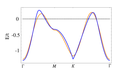
which will be used to perform the open boundary calculation in next section. In the 4-orbital model, we choose the parameters as: , , , , , . Then, we fit the one-orbital model on a triangular lattice to obtain the hopping parameters: , , , and the chemical potential . The band structures obtained by the one-orbital model and 4-orbital minimal model are shown in Fig. 5 by orange and blue lines, respectively.
.7 Topological properties of superconducting state
As discussed in previous sections and the main text, the nodal superconducting order parameters with nonzero in-plane magnetic moments can be constructed by combining order parameters from different irreps. The superconducting order parameter can generally be expressed as:
| (39) |
The parameters and depend on the relative amplitudes between superconducting order parameters belonging to different irreps. We choose without loss of generality. In addition, as discussed in the main text, the intrinsic polarization of the pairing state is determined by the decoupling coefficient and can be characterized by the parameter . The highest transition temperature corresponds to the , which we choose to be .
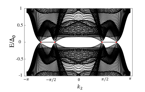
We calculate the spectrum structure under the open boundary condition, there are Majorana zero modes between the nodes of the superconductivity as shown in Fig. 6. The coordinates of these nodes are .
The winding number at a certain can be calculated by equation:
| (40) |
where is chiral operator: . However, the equation is available only when can not be block-diagonal. If the Hamiltonian can be block-diagonal, we can find two different chiral operators and , which yield two different winding numbers.
When there is no magnetic field, the total BdG Hamiltonian can be expressed as:
| (41) |
where we rewrite the d-vector as: , and with are identity matrix () and Pauli matrices (). We then find a unitary transformation matrix which can make the Hamiltonian to be block-diagonal.
| (46) |
where .
The block-diagonal Hamiltonian can be expressed as:
| (47) |
where these two matrices are:
| (48) |
and
| (49) |
Here, two chiral symmetry operators are:
| (50) | |||
where . For these two blocks, the chiral symmetry is both . It’s convenient to transform these two chiral symmetry operators to be block-diagonal:
| (51) | |||
The Eq. (51) indicates that one of the total winding numbers is the sum of the two block winding numbers, while the other is the difference between the two block winding numbers. For positive , the winding number of and between point nodes can be expressed as:
| (52) | |||
and
| (53) |
respectively.
Then we apply a magnetic field along the x-axis, . In BdG Hamiltonian, this magnetic field can be expressed as: , which preserve the effective time-reversal symmetry: () and particle-hole symmetry: . Thus, it preserves the chiral symmetry: . The time reversal and particle-hole symmetry are defined by:
| (54) | |||
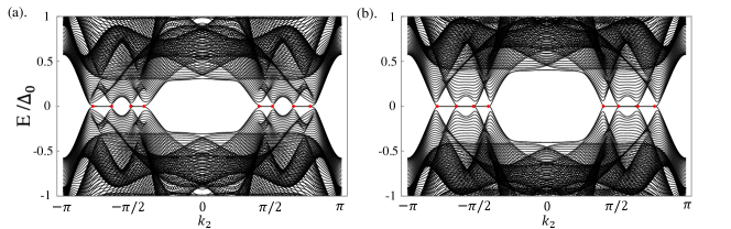
respectively. Each point node on -axis will split into two. We perform the open boundary calculation and obtain the spectral structure illustrated in Fig. 7.

The coordinates of the point nodes are , , , , , , and , respectively. The winding number can also be calculated:
| (55) | |||
When the magnetic field is along the y-axis, the open boundary spectrum is shown in Fig.8.
The magnetic field along the y-axis in BdG Hamiltonian can be expressed as: , which preserves the effective time-reversal symmetry: () and particle-hole symmetry: .
For each point, when considering the in-plane magnetic field, although the effective magnetic field is -dependent, it can only have - and - components, as the SOPC is of the Rashba type. Therefore, the effective time-reversal symmetry, particle-hole symmetry, and chiral symmetry remain unchanged, even in the presence of a -dependent effective magnetic field. We can adopt a gauge-independent approach to calculate the winding number in the presence of a -dependent effective magnetic field, described as follows: The existence of the chiral symmetry ensures the Hamiltonian can be off-block-diagonalized as:
| (56) |
The unitary matrix satisfy the condition:
| (57) |
The gauge-independent equation of the winding number for each is:
| (58) |
where we use the equation: . The result is the same as the expression given in Eq. (55).
.8 Method of tunneling spectra calculation
The tunneling conductance between the scanning tunneling microscope (STM) lead and the kagome superconductor is calculated using the scattering matrix approach:
| (59) |
where is the Fermi distribution function. An electron coming from the STM lead will be scattered when it tunnels into the Kagome superconductor. The reflection matrices in Eq. (59) can be understood as for an incoming electron, there is a chance to be scattered back as an electron and a chance to be scattered back as a hole. Near zero bias, the Andreev reflection process will be resonant for the edge Majorana flat band. Technically, the reflection matrix can be calculated from the recursive Green’s function method:
| (60) |
Here, , the broadening function , where is the self energy of semi-infinite STM lead. is the retarded Green’s function. labels the position where STM tunnels.
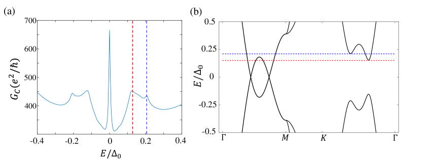
Besides the zero-bias peak, additional peaks in the tunneling conductance arise from the two-gap behavior of the superconducting states, as shown in Fig. 9 (a). When compared to the quasiparticle band structure of the BdG Hamiltonian which is shown in Fig. 9 (b), we find that the energy of the additional peaks correlates with the energy of the quasiparticle band bottom, which is determined by the amplitudes of the gaps on different Fermi surfaces.