Observer-based Event-triggered Boundary Control of the One-phase Stefan Problem
Abstract
This paper provides an observer-based event-triggered boundary control strategy for the one-phase Stefan problem using the position and velocity measurements of the moving interface. The infinite-dimensional backstepping approach is used to design the underlying observer and controller. For the event-triggered implementation of the continuous-time observer-based controller, a dynamic event triggering condition is proposed. The triggering condition determines the times at which the control input needs to be updated. In between events, the control input is applied in a Zero-Order-Hold fashion. It is shown that the dwell-time between two triggering instances is uniformly bounded below excluding Zeno behavior. Under the proposed event-triggered boundary control approach, the well-posedness of the closed-loop system along with certain model validity conditions is provided. Further, using Lyapunov approach, the global exponential convergence of the closed-loop system to the setpoint is proved. A simulation example is provided to illustrate the theoretical results.
keywords:
Backstepping control design, event-triggered control, moving boundaries, output-feedback, Stefan problem.1 Introduction
In recent decades, the study of Stefan-type moving boundary problems driven by parabolic equations has found a new momentum due to the expansion of its interests into thriving areas of research such as additive manufacturing (Petrus \BOthers., \APACyear2017; Chen \BOthers., \APACyear2020), cyrosurgical operations (Rabin \BBA Shitzer, \APACyear1997), modeling of tumor growth (Friedman \BBA Reitich, \APACyear1999), and information diffusion in social media (Lei \BOthers., \APACyear2013). The mathematical formulation of the classical one-phase Stefan problem for a monocomponent two phase material involves a diffusion partial differential equation (PDE) in cascade with an ordinary differential equation (ODE). The PDE describes the thermal expansion of one phase along its dynamic spatial domain whereas the ODE captures the dynamics of the moving interface between the two phases (Rubinstein, \APACyear1979).
The control of the Stefan problem deals with the stabilization of the temperature profile and the moving interface to a desired setpoint. During the past decade, inspired by the seminal work (Dunbar \BOthers., \APACyear2003) on boundary control of the Stefan problem, numerous works have made contributions to tackle this challenging moving boundary PDE control problem (Petrus \BOthers., \APACyear2012; Chen \BOthers., \APACyear2020; Petrus \BOthers., \APACyear2017; Chen \BOthers., \APACyear2019; Maidi \BBA Corriou, \APACyear2014; Koga, Diagne\BCBL \BBA Krstic, \APACyear2018; Koga, Bresch-Pietri\BCBL \BBA Krstic, \APACyear2020; Koga, Karafyllis\BCBL \BBA Krstic, \APACyear2018; Ecklebe \BOthers., \APACyear2021). An enthalpy-based full-state feedback boundary controller is proposed in (Petrus \BOthers., \APACyear2012) to ensure the asymptotic convergence of the closed-loop system to the setpoint. Compensating for the effect of input hysteresis, the authors of (Chen \BOthers., \APACyear2019) and (Chen \BOthers., \APACyear2020) develop full-state feedback and output feedback designs for the control of the Stefan problem, respectively. Using a geometric control approach, Maidi \BBA Corriou (\APACyear2014) achieves exponential stability of the closed-loop system for the one-phase Stefan problem via Lyapunov analysis. In recent years, Koga and coauthors have addressed the control of the Stefan problem in both theoretical settings (Koga, Diagne\BCBL \BBA Krstic, \APACyear2018; Koga \BBA Krstic, \APACyear2020) and application settings (Koga, Straub\BCBL \BOthers., \APACyear2020; Koga \BBA Krstic, \APACyear2020) using the infinite-dimensional backstepping control approach which has been instrumental in the control of a wide variety of PDEs (Krstic \BBA Smyshlyaev, \APACyear2008). For the one-phase Stefan problem, the pioneering contribution (Koga, Diagne\BCBL \BBA Krstic, \APACyear2018) discusses a full-state feedback control design along with robustness guarantees to parameter uncertainties, an observer design, and the corresponding output feedback control design under both Dirichlet and Neumann boundary actuations via backstepping approach, ensuring the exponential stability of the closed-loop system in -norm.
In (Koga \BOthers., \APACyear2021), the authors consider the Zero-Order-Hold (ZOH) implementation of the full-state feedback continuous-time stabilizing controller introduced in (Koga, Diagne\BCBL \BBA Krstic, \APACyear2018), leading to an aperiodic sampled-data control approach for the one-phase Stefan problem. Aperiodic sampled-data control strategies, which rely on nonuniform sampling schedules, are quite appealing as they point towards efficient use of limited hardware, software, and communication resources. In a relatively recent survey paper (Hetel \BOthers., \APACyear2017), comprehensive and relevant insights are provided into aperiodic sampled-data controller design, as well as limitations and challenges in their practical implementation. Although nonuniform sampling schedules in aperiodic sampled-data control offer increased flexibility, designers still have to manually select a schedule that adheres to the maximum allowable sampling diameter. This selection remains independent of the closed-loop system state, rendering the decision-making process open-loop. Event-triggered control strategies, on the other hand, provide a systematic solution to this drawback by bringing feedback to the sampling process. An event-triggered system transmits the system’s states/outputs to a controller/actuator when the freshness in the sample exceeds an appropriate threshold involving the current state of the closed-loop system (Heemels \BOthers., \APACyear2012). Only at the event times is the feedback loop closed, and between successive event times, the control is executed in an open-loop fashion. There have been numerous contributions during the past decade introducing event-triggered control strategies to control for PDE systems (Espitia, \APACyear2020; Katz \BOthers., \APACyear2020; Espitia \BOthers., \APACyear2021; Diagne \BBA Karafyllis, \APACyear2021; Rathnayake \BOthers., \APACyear2021, \APACyear2022; Wang \BBA Krstic, \APACyear2021; Rathnayake \BBA Diagne, \APACyear2022), to name a few. For 22 linear hyperbolic systems, an output feedback event-triggered boundary control strategies relying on dynamic triggering conditions is proposed in (Espitia, \APACyear2020). The authors of (Espitia \BOthers., \APACyear2021) propose a full-state feedback event-triggered boundary control approach for reaction-diffusion PDEs with Dirichlet boundary conditions using ISS properties and small gain arguments. Using dynamic event-triggering conditions, the works (Rathnayake \BOthers., \APACyear2021) and (Rathnayake \BOthers., \APACyear2022) develop output feedback control strategies for a class of reaction-diffusion PDEs under anti-collocated and collocated boundary sensing and actuation, respectively. A full-state feedback event-triggered boundary control strategy for the one-phase Stefan problem is proposed in (Rathnayake \BBA Diagne, \APACyear2022) using a static triggering condition.
This paper considers the output feedback boundary control of the one-phase Stefan problem using the position and velocity measurements of the moving interface. We propose an observer-based event-triggered boundary control strategy using a dynamic triggering condition under which we show that the closed-loop system is free from Zeno phenomenon. To the best of our knowledge, this work is the first to present an observer-based event-triggered boundary control approach for moving boundary type problems. In (Koga, Makihata\BCBL \BOthers., \APACyear2020), the authors propose a sampled-data observer-based boundary control design for the one-phase Stefan problem, yet with no theoretical guarantees. At event-times dictated by the proposed triggering condition, the continuous-time observer-based boundary control law derived in (Koga, Diagne\BCBL \BBA Krstic, \APACyear2018) is computed and applied to the plant in a ZOH fashion. The dynamic event-trigger makes use of a dynamic variable that depends on some information of the current states of the closed-loop system and the actuation deviation between the continuous-time boundary feedback and the event-triggered boundary control. We also prove that the closed-loop system is well-posed satisfying certain model validity conditions and globally exponentially converges to the setpoint subject to the proposed event-triggered control. The present work differs from (Rathnayake \BOthers., \APACyear2021, \APACyear2022) in that this paper involves a moving boundary making the Lyapunov analysis substantially different. Moreover, the Lyapunov candidate function involves the -norm of the observer error target system unlike in (Rathnayake \BOthers., \APACyear2021, \APACyear2022) where the -norm is sufficient. As opposed to (Rathnayake \BOthers., \APACyear2021, \APACyear2022), dwell-times between consecutive events in the Stefan problem has to be upper-bounded to maintain the positivity of the control input. Thus, careful design of the event-triggering mechanism is required to ensure that the minimal dwell-time is smaller than the largest dwell-time, otherwise, the well-posedness of the closed-loop system fails to exist.
The paper is organized as follows. Section 2 describes the one-phase Stefan problem and Section 3 presents the continuous-time observer-based backstepping boundary control and its emulation. In section 4, we introduce the event-triggered boundary control approach and present the main results of the paper. We conduct simulations in Section 5 and conclude the paper in Section 6.
Notation: is the nonnegative real line whereas is the set of natural numbers including zero. and respectively denote the right and left limit at time . Let be given. denotes the profile of at certain , i.e., , for all . By we denote -norm. and with being an integer respectively denote modified Bessel and (nonmodified) Bessel functions of the first kind.
2 Description of the One-phase Stefan Problem
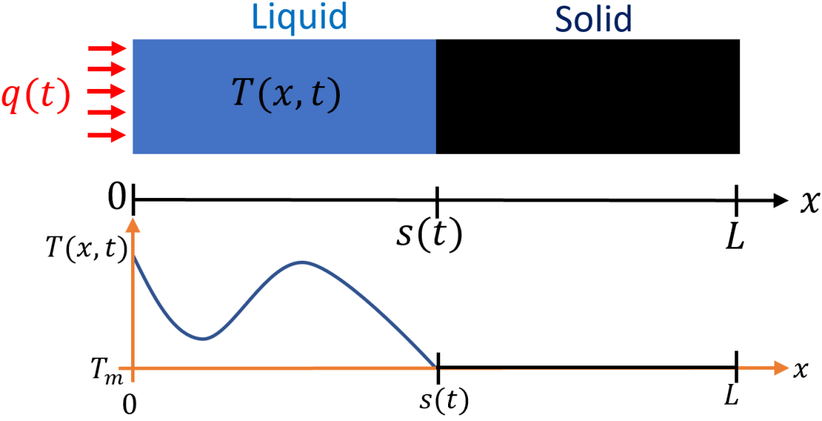
Let us consider a physical model that describes the melting or solidification process in a pure one-component material of length in one dimension. The position at which the phase transition occurs divides the domain into two time-varying sub-domains; the interval containing the liquid phase, and the interval containing the solid phase. The dynamics of the position of the liquid-solid interface is driven by a heat flux entering through the boundary at (the fixed boundary of the liquid phase). The heat equation coupled with the dynamics that describes the moving boundary is used to characterize the heat propagation in the liquid phase and the phase transition. Fig. 1 illustrates this configuration.
Under the assumption that the temperature in the liquid phase is not lower than the melting temperature of the material, the conservation of energy and heat conduction laws can be used to derive the following PDE-ODE cascade system known as the one-phase Stefan Problem.
| (1) |
with the boundary conditions
| (2) | ||||
| (3) |
and the initial values
| (4) |
where and are the liquid phase distributed temperature, applied heat flux, the liquid density, the liquid heat capacity, and the liquid heat conductivity, respectively. By considering the local energy balance at the liquid-solid interface , the following ODE associated with the time-evolution of the spatial domain can be obtained:
| (5) |
where is the latent heat of fusion.
The validity of the physical model (1)-(5) relies on two physical conditions (Koga \BOthers., \APACyear2019):
| (6) |
| (7) |
The first condition implies that the liquid phase should not be frozen to the solid phase from the boundary . The second condition implies that the material should not be completely melted or frozen to single phase through the disappearance of the other phase.
To be consistent with the conditions (6) and (7), we make the following assumptions on the initial data:
Assumption 1.
for all and is continuously differentiable in .
The well-posedness of the solution of the one-phase Stefan problem (1)-(5) has been presented in (Cannon \BBA Primicerio, \APACyear1971) and Lemma 1 in (Koga \BOthers., \APACyear2019) which we state as follows:
3 Observer-based Backstepping Boundary Control and Emulation
The steady-state solution of the system (1)-(5) with zero input delivers a uniform temperature distribution and a constant interface position determined by initial data. In (Koga, Diagne\BCBL \BBA Krstic, \APACyear2018), the authors proposed a continuous-time observer-based backstepping boundary controller using and (or equivalently due to (5)) as the available measurements to exponentially stabilize the interface position at a desired reference setpoint through the design of as
| (9) |
where is the control gain and and are reference error variables defined as
| (10) | ||||
| (11) |
Here, is the observer state which satisfies
| (12) |
for and
| (13) | ||||
| (14) |
with being the observer gain given by
| (15) |
for .
We aim to stabilize the closed-loop system containing the plant (1)-(5) and the observer (12)-(15) while sampling the continuous-time controller given by (9) at a certain sequence of time instants . These time instants will be fully characterized later via a dynamic event-trigger. The control input is held constant between two consecutive time instants. Therefore, we define the control input for all as
| (16) |
Accordingly, the boundary conditions (3) and (14) are modified as follows:
| (17) |
| (18) |
for . Let the observer error state be defined as
| (19) |
Therefore, considering (1),(2),(12),(13),(17),(18), we can obtain that
| (20) | ||||
| (21) | ||||
| (22) |
for all . In (Koga, Diagne\BCBL \BBA Krstic, \APACyear2018), the authors show that, subject to the following invertible backstepping transformation
| (23) |
where
| (24) |
for , the observer error system (20)-(22) with the gain chosen as in (15) gets transformed into the following globally -exponentially stable observer error target system
| (25) | ||||
| (26) | ||||
| (27) |
The inverse transformation of (23) is given by
| (28) |
where
| (29) |
for . Considering (10),(12),(13), and (18), we can obtain that -system satisfies
| (30) | ||||
| (31) | ||||
| (32) |
whereas considering (5),(10),(11),(19), we can show that the dynamics of satisfies
| (33) |
Let us consider the following backstepping transformation on as in (Koga \BOthers., \APACyear2019),
| (34) |
where
| (35) |
It can be shown that the backstepping transformation (34),(35) transforms system (30)-(33) into the following system valid for :
| (36) | ||||
| (37) | ||||
| (38) | ||||
| (39) |
where
| (40) |
and
| (41) |
for .
4 Observer-based Event-triggered Boundary Control
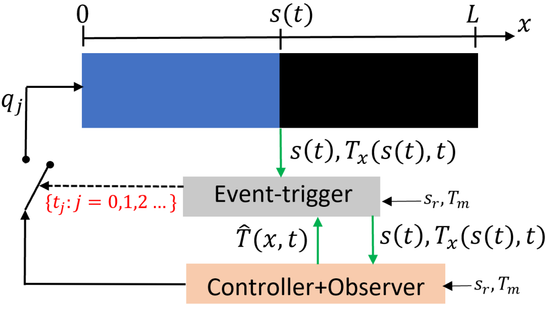
Next we present the observer-based event-triggered boundary control approach for the one-phase Stefan problem. The closed-loop system consisting of the plant, the observer-based controller, and the event-trigger is shown in Fig. 2.
Definition 1.
Let be several design parameters. Further, let be the control gain in (16). The observer-based event-triggered boundary control strategy consists of two components:
-
1.
The event-trigger: The set of event times is generated via the following rule with :
(45) where
(46) Here defined in (41) for all for all is the difference between the continuous time control input and the event-triggered control input, and satisfies the ODE
(47) for all with and .
-
2.
The control action: The boundary feedback control law is given by (16).
Lemma 2.
Along with Assumption 1, let us suppose the following Lipschitz continuity of holds,
| (48) |
where is assumed to be known. For any initial temperature estimation , any gain parameter of the observer , and any setpoint , suppose that the following relations are satisfied respectively,
| (49) | ||||
| (50) | ||||
| (51) |
where the parameters and satisfy . Then, the event-triggered boundary control approach in Definition 1 generates positive heat, i.e., for such that where
| (52) |
with being the set of event times. Moreover, the closed-loop system containing the plant (1),(2),(4),(5),(16),(17) and the observer (12),(13),(15),(16),(18) has a unique solution satisfying the conditions (6)-(8) for .
Proof: For where , differentiating (9) along the solution of (30)-(33), we can obtain that
Subject to the conditions (49) and (50), following Lemma 3 and 4 in (Koga, Diagne\BCBL \BBA Krstic, \APACyear2018) which make use of Maximum principle and Hopf’s lemma, one can show that . Note from (15) that for . Thus, we can obtain that for which we integrate in to obtain
| (53) |
We use this recursively to derive that
| (54) |
One can easily show that when the conditions (49) and (51) are met. Furthermore, under the event-triggered boundary control approach in Definition 1, it is ensured that . Therefore, we have that for all such that . Thus, recalling Lemma 1, we can conclude that the plant (1),(2),(4),(5),(16),(17) has a unique solution satisfying the conditions (6) and (8) in the interval . The observer error system (20)-(22) has a unique solution due to the transformation (23) and as the observer error target system (25)-(27) admits a unique solution. Thus, the observer PDE (12),(13),(15),(16),(18) also admits a unique solution in the interval due to (19). Again, subject to the conditions (49) and (50), one can show that as in Lemma 3 and 4 in (Koga, Diagne\BCBL \BBA Krstic, \APACyear2018). Thus, considering (6),(10),(19), we can verify that . Further, note from (53) that for . Thus, considering (9), we can show that for which in combination with (8) and (11) leads to the property (7) for . ∎
Proof: According to Definition 1, the triggering of events guarantee that . This inequality in combination with (47) yields:
| (55) |
for and such that where is given by (52). Thus, considering the time-continuity of , we can obtain the following estimate:
| (56) |
for all . From Definition 1, we have that . Therefore, it follows from (56) that for all . Again using (56) on , we can show that for all . Applying the same reasoning successively to the future intervals, it can be shown that for . ∎
Lemma 4.
Proof: For , differentiating given by (41) along the solution of (30)-(33) and using (41), we can obtain that
| (59) |
Using Cauchy-Schwarz inequality and Young’s inequality along with the fact that , we can obtain from (59) that
| (60) |
for all and such that where is given by (52). ∎
4.0.1 Avoidance of Zeno behavior
Theorem 1.
Let be chosen such that
| (61) |
where is the controller gain in (16). Then, under the observer-based event-triggered boundary control in Definition 1, with chosen as
| (62) |
where given by (58), there exists such that for all and any choice of admissible initial conditions and , and desired liquid-solid interface which satisfy Assumption 1 and the conditions (48)-(51).
Proof: Let us assume that an event has occurred at for some such that where is given by (52). Furthermore, without loss of generality, let us assume that the set given by (46) is not empty (otherwise the next event time is ). Therefore, according to (45), we have that
| (63) |
In this case, we have that for and . Further, from Lemma 3, we have that for .
Let us define the function
| (64) |
Note that is continuous in and . A lower bound for the dwell-times is given by the time it takes for the function to go from to where , which holds since . Therefore, by the intermediate value theorem, there exists a such that and for . The time derivative of on is given by
| (65) |
From Young’s inequality, we have that
| (66) |
Using Lemma 4 and (47), we can show that
| (67) |
Let us choose as in (62), where are given by (58). Also note that the last term in the right hand side of (67) is negative. Therefore, we have
| (68) |
which we rewrite to obtain
| (69) |
Rearranging the terms in (69) lead to
| (70) |
where
| (71) | ||||
| (72) | ||||
| (73) |
By the Comparison principle, it follows that the time needed for to go from to is at least
| (74) |
Therefore, . As , we can conclude that . Note from (74), (73), and (61) that where is the maximum dwell-time allowed by the definition of the event-trigger in Definition 1. Furthermore, the set of event-times is a strictly increasing sequence to infinity, i.e., as . ∎
4.0.2 Exponential Convergence
Theorem 2.
Consider the closed-loop system containing the plant (1),(2),(4),(5),(16),(17) and the observer (12),(13),(15),(16),(18) subject to Assumption 1 and conditions (48)-(51). In Definition 1, let us select the event-trigger parameters as follows. Let be design parameters, and let us choose the parameters as in (62). Further, let us choose such that
| (75) |
where is any positive parameter that satisfies
| (76) |
with given by (44) and in (35) chosen to satisfy
| (77) |
where
| (78) |
and is the positive solution of the quadratic equation
| (79) |
Then, subject to the event-triggered boundary control apprach in Definition 1, the closed-loop system has a unique solution satisfying (6)-(8) and exponentially converges to zero, i.e., as where , and .
Proof: Theorem 1 ensures the existence of an increasing sequence as it is proven that for any . Therefore, considering Lemma 2, we can show that the closed-loop system has a unique solution satisfying (6)-(8) for all . Now let us show the exponential convergence of the closed-loop system.
Let us consider a positive definite function involving the system (36)-(39) and (25)-(27) as follows:
| (80) |
where . Differentiating (80) along the solution of (36)-(39),(25)-(27) in and using integration by parts and (42), we can obtain that
| (81) |
From (43), it follows that from which we can obtain that Now, recalling from (77) that , we can show that
Further, we can write that from which we can obtain that . Thus, using Cauchy-Schwarz inequalities on (81) and noting that from Lemma 2, we can obtain that
| (82) |
where are some positive constants and
for given by (40). Using Poincare and Agmon inequalities together with the fact that for the system (36)-(38), we can obtain that
| (83) | ||||
| (84) |
Substituting and in (82) with (83) and (84), we can obtain
| (85) |
Let us choose . Then, we can rewrite (85) as
| (86) |
Then, recalling from (77) that letting where , and substituting with (83), we can obtain from (86) that
| (87) |
Above we have used the fact that . Let us define
Then, we have that and
for Therefore, we have such that for and . Since (see (77)), we have that . Thus, we can write from (87) that
| (88) |
Let us consider the following Lyapunov function recalling from Lemma 3 that for :
| (89) |
Taking the time derivative of (89) and using (88), we can write that
| (90) |
Noting that from Lemma 2, using (80) along with the dynamics of given by (47), we can obtain from (90) that
| (91) |
where
| (92) |
Using Cauchy-Schwarz inequality and Young’s inequality along with the fact that , we can obtain from (42) that
| (93) |
Noting that and that , we can obtain from (91) that
| (94) |
Let us define
| (95) |
and
| (96) |
Recall that due to the choice of as in (77)-(79). Considering (76), we can show that . Let us select such that Then, recalling (75), we can write from (94) that
| (97) |
where
| (98) |
Consider the following functional
| (99) |
Taking the time derivative of (99) for with the aid of (97), we can deduce Via integration and considering (99) and the fact that , we can obtain
Thus, using the transformations (23),(28),(34),(42), Young’s and Cauchy-Schwarz inequalities, we can show that there exists a constant such that
| (100) | ||||
| (101) |
∎
Remark 1.
(Selection of the event-trigger parameters ) The parameters are chosen to satisfy (62) with being treated as a free parameter which can be chosen to scale up/down the values of as required, and chosen to satisfy (61). The parameter is chosen as in (75). The parameter is also a free parameter, which can be used to adjust the convergence rate of the dynamic variable .
5 Numerical Simulations and Discussion
We carry out simulations for the one-phase Stefan problem considering a cylinder of paraffin with length cm whose physical parameters are as follows: kg.mJ.gJ.gCCW.m-1. We use a semi-implicit numerical scheme relying on the so-called boundary immobilization method (Koleva \BBA Valkov, \APACyear2010). A uniform step size of is used for the space variable and a uniform step size of s is used for the time variable. The setpoint and the initial values are chosen as cm, cm, and . The observer gain is chosen as . Note that under these choices of and , there exists constants such that the conditions (48)-(51) are satisfied. The control gain in (16) is chosen as . The parameter in (35) is chosen as such that (77)-(79) are satisfied. The parameters for the event-trigger are chosen as follows: . Note that the above choices of satisfy (62) when . The chosen satisfies (75) when .
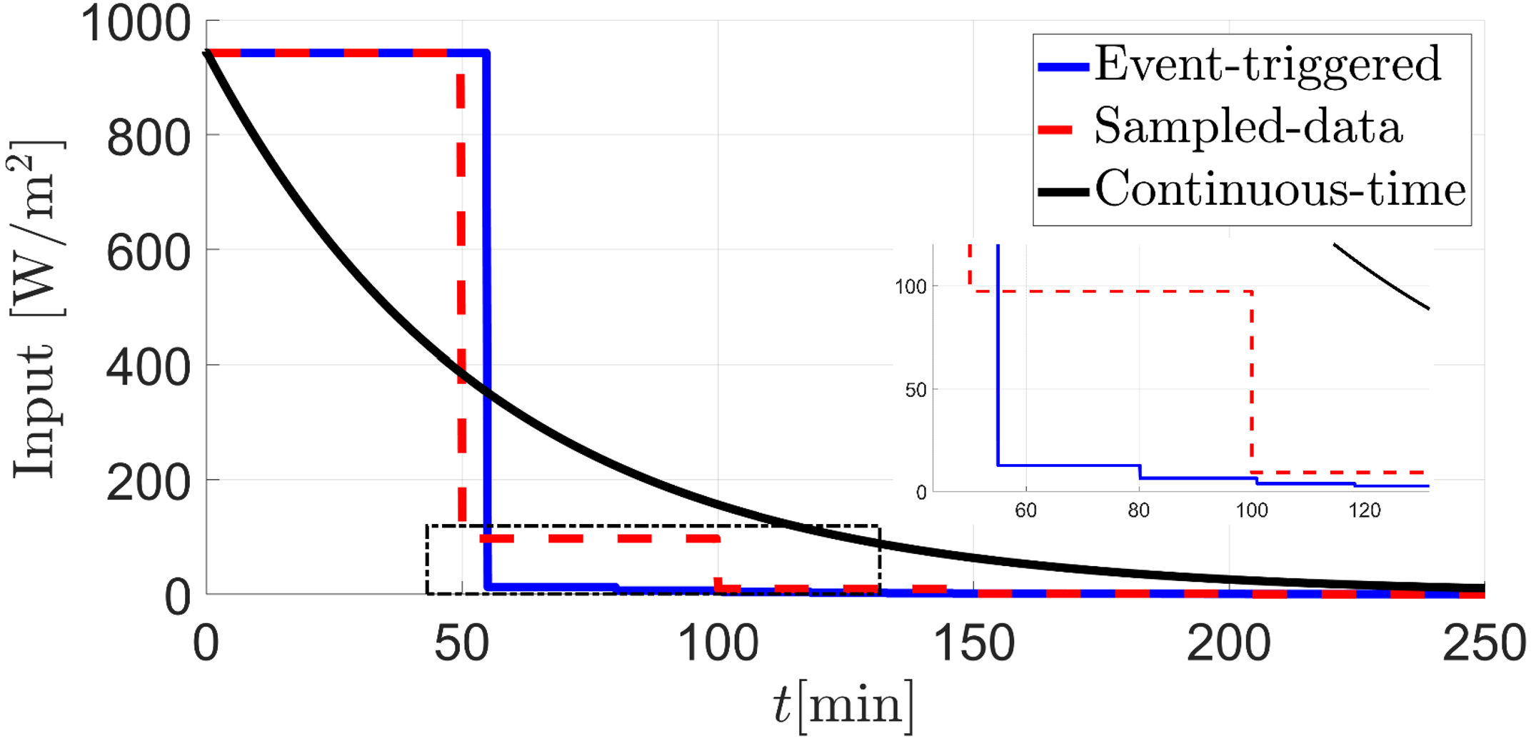
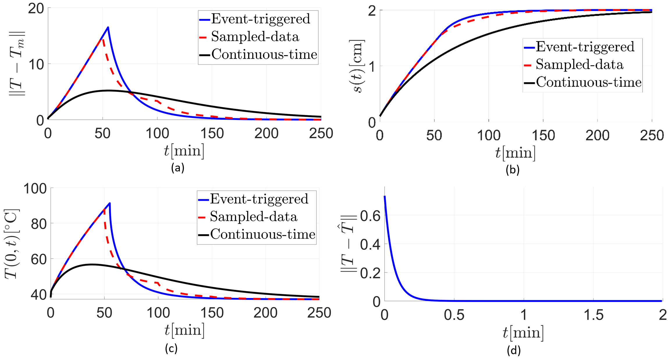
The control inputs under even-triggered, sampled-data, and continuous-time control are shown in Fig. 3. We can observe that event-triggered control eliminates the necessity of continuous control updates. Fig. 4 illustrates the time evolution of various closed-loop system signals under the proposed event-based boundary control. The time responses of , boundary temperature [∘C], and are shown in Fig. 4(a), Fig. 4(c), and Fig. 4(d), respectively. It can be observed that, and as and for all . Fig. 4(b) shows the the time evolution of the interface position under the proposed event-based boundary control. The interface position converges to the setpoint monotonically without overshooting (which also confirms that ).
6 Conclusion
In this paper, we have proposed an observer-based event-triggered boundary control strategy for the one-phase Stefan problem using the infinite-dimensional backstepping approach. We have used a dynamic event-triggering condition to determine the time instances when the control input needs to be updated. Under the observer-based event-triggered control strategy, we have proved the existence of a uniform minimal dwell-time, which excludes Zeno behavior from the closed-loop system. Furthermore, we have proved the well-posedness of the closed-loop system along with the model validity conditions. Finally, we have shown that the proposed control approach exponentially converges the closed-loop system to the setpoint. In our future work, we will consider the observer-based event-triggered boundary control of the two-phase Stefan problem.
Disclosure statement
The authors hereby declare that they have no relevant financial or non-financial competing interests in relation to this manuscript submitted to the journal.
References
- Cannon \BBA Primicerio (\APACyear1971) \APACinsertmetastarcannon1971remarks{APACrefauthors}Cannon, J.\BCBT \BBA Primicerio, M. \APACrefYearMonthDay1971. \BBOQ\APACrefatitleRemarks on the one-phase Stefan problem for the heat equation with the flux prescribed on the fixed boundary Remarks on the one-phase Stefan problem for the heat equation with the flux prescribed on the fixed boundary.\BBCQ \APACjournalVolNumPagesJournal of Mathematical Analysis and Applications352361–373. \PrintBackRefs\CurrentBib
- Chen \BOthers. (\APACyear2019) \APACinsertmetastarchen2019enthalpy{APACrefauthors}Chen, Z., Bentsman, J.\BCBL \BBA Thomas, B\BPBIG. \APACrefYearMonthDay2019. \BBOQ\APACrefatitleEnthalpy-based Full-State Feedback Control of the Stefan Problem with Hysteresis Enthalpy-based full-state feedback control of the Stefan problem with hysteresis.\BBCQ \BIn \APACrefbtitle2019 IEEE 58th Conference on Decision and Control (CDC) 2019 ieee 58th conference on decision and control (cdc) (\BPGS 4035–4040). \PrintBackRefs\CurrentBib
- Chen \BOthers. (\APACyear2020) \APACinsertmetastarchen2020enthalpy{APACrefauthors}Chen, Z., Bentsman, J.\BCBL \BBA Thomas, B\BPBIG. \APACrefYearMonthDay2020. \BBOQ\APACrefatitleEnthalpy-based Output Feedback Control of the Stefan Problem with Hysteresis Enthalpy-based output feedback control of the Stefan problem with hysteresis.\BBCQ \BIn \APACrefbtitle2020 American Control Conference (ACC) 2020 american control conference (acc) (\BPGS 2661–2666). \PrintBackRefs\CurrentBib
- Diagne \BBA Karafyllis (\APACyear2021) \APACinsertmetastardiagne2021event{APACrefauthors}Diagne, M.\BCBT \BBA Karafyllis, I. \APACrefYearMonthDay2021. \BBOQ\APACrefatitleEvent-triggered boundary control of a continuum model of highly re-entrant manufacturing systems Event-triggered boundary control of a continuum model of highly re-entrant manufacturing systems.\BBCQ \APACjournalVolNumPagesAutomatica134109902. \PrintBackRefs\CurrentBib
- Dunbar \BOthers. (\APACyear2003) \APACinsertmetastardunbar2003motion{APACrefauthors}Dunbar, W\BPBIB., Petit, N., Rouchon, P.\BCBL \BBA Martin, P. \APACrefYearMonthDay2003. \BBOQ\APACrefatitleMotion planning for a nonlinear Stefan problem Motion planning for a nonlinear Stefan problem.\BBCQ \APACjournalVolNumPagesESAIM: Control, Optimisation and Calculus of Variations9275–296. \PrintBackRefs\CurrentBib
- Ecklebe \BOthers. (\APACyear2021) \APACinsertmetastarecklebe2021toward{APACrefauthors}Ecklebe, S., Woittennek, F., Frank-Rotsch, C., Dropka, N.\BCBL \BBA Winkler, J. \APACrefYearMonthDay2021. \BBOQ\APACrefatitleToward model-based control of the vertical gradient freeze crystal growth process Toward model-based control of the vertical gradient freeze crystal growth process.\BBCQ \APACjournalVolNumPagesIEEE Transactions on Control Systems Technology301384–391. \PrintBackRefs\CurrentBib
- Espitia (\APACyear2020) \APACinsertmetastarespitia2020observer{APACrefauthors}Espitia, N. \APACrefYearMonthDay2020. \BBOQ\APACrefatitleObserver-based event-triggered boundary control of a linear 2 2 hyperbolic systems Observer-based event-triggered boundary control of a linear 2 2 hyperbolic systems.\BBCQ \APACjournalVolNumPagesSystems & Control Letters138104668. \PrintBackRefs\CurrentBib
- Espitia \BOthers. (\APACyear2021) \APACinsertmetastarespitia2021event{APACrefauthors}Espitia, N., Karafyllis, I.\BCBL \BBA Krstic, M. \APACrefYearMonthDay2021. \BBOQ\APACrefatitleEvent-triggered boundary control of constant-parameter reaction–diffusion PDEs: A small-gain approach Event-triggered boundary control of constant-parameter reaction–diffusion PDEs: A small-gain approach.\BBCQ \APACjournalVolNumPagesAutomatica128109562. \PrintBackRefs\CurrentBib
- Friedman \BBA Reitich (\APACyear1999) \APACinsertmetastarfriedman1999analysis{APACrefauthors}Friedman, A.\BCBT \BBA Reitich, F. \APACrefYearMonthDay1999. \BBOQ\APACrefatitleAnalysis of a mathematical model for the growth of tumors Analysis of a mathematical model for the growth of tumors.\BBCQ \APACjournalVolNumPagesJournal of mathematical biology383262–284. \PrintBackRefs\CurrentBib
- Heemels \BOthers. (\APACyear2012) \APACinsertmetastarheemels2012introduction{APACrefauthors}Heemels, W., Johansson, K\BPBIH.\BCBL \BBA Tabuada, P. \APACrefYearMonthDay2012. \BBOQ\APACrefatitleAn introduction to event-triggered and self-triggered control An introduction to event-triggered and self-triggered control.\BBCQ \BIn \APACrefbtitle2012 51st IEEE Conference on Decision and Control (CDC) 2012 51st ieee conference on decision and control (cdc) (\BPGS 3270–3285). \PrintBackRefs\CurrentBib
- Hetel \BOthers. (\APACyear2017) \APACinsertmetastarLaurentiu17{APACrefauthors}Hetel, L., Fiterand, C., Omran, H., Seuret, A., Fridman, E., Richard, J\BHBIP.\BCBL \BBA Niculescu, S\BPBII. \APACrefYearMonthDay2017. \BBOQ\APACrefatitleRecent developments on the stability of systems with aperiodic sampling: An overview Recent developments on the stability of systems with aperiodic sampling: An overview.\BBCQ \APACjournalVolNumPagesAutomatica76309-335. \PrintBackRefs\CurrentBib
- Katz \BOthers. (\APACyear2020) \APACinsertmetastarkatz2020boundary{APACrefauthors}Katz, R., Fridman, E.\BCBL \BBA Selivanov, A. \APACrefYearMonthDay2020. \BBOQ\APACrefatitleBoundary delayed observer-controller design for reaction-diffusion systems Boundary delayed observer-controller design for reaction-diffusion systems.\BBCQ \APACjournalVolNumPagesIEEE Transactions on Automatic Control. \PrintBackRefs\CurrentBib
- Koga, Bresch-Pietri\BCBL \BBA Krstic (\APACyear2020) \APACinsertmetastarkoga2020delay{APACrefauthors}Koga, S., Bresch-Pietri, D.\BCBL \BBA Krstic, M. \APACrefYearMonthDay2020. \BBOQ\APACrefatitleDelay compensated control of the Stefan problem and robustness to delay mismatch Delay compensated control of the Stefan problem and robustness to delay mismatch.\BBCQ \APACjournalVolNumPagesInternational Journal of Robust and Nonlinear Control3062304–2334. \PrintBackRefs\CurrentBib
- Koga, Diagne\BCBL \BBA Krstic (\APACyear2018) \APACinsertmetastarkoga2018control{APACrefauthors}Koga, S., Diagne, M.\BCBL \BBA Krstic, M. \APACrefYearMonthDay2018. \BBOQ\APACrefatitleControl and state estimation of the one-phase Stefan problem via backstepping design Control and state estimation of the one-phase Stefan problem via backstepping design.\BBCQ \APACjournalVolNumPagesIEEE Transactions on Automatic Control642510–525. \PrintBackRefs\CurrentBib
- Koga, Karafyllis\BCBL \BBA Krstic (\APACyear2018) \APACinsertmetastarkoga2018input{APACrefauthors}Koga, S., Karafyllis, I.\BCBL \BBA Krstic, M. \APACrefYearMonthDay2018. \BBOQ\APACrefatitleInput-to-state stability for the control of Stefan problem with respect to heat loss at the interface Input-to-state stability for the control of Stefan problem with respect to heat loss at the interface.\BBCQ \BIn \APACrefbtitle2018 Annual American Control Conference (ACC) 2018 annual american control conference (acc) (\BPGS 1740–1745). \PrintBackRefs\CurrentBib
- Koga \BOthers. (\APACyear2019) \APACinsertmetastarkoga2019sampled{APACrefauthors}Koga, S., Karafyllis, I.\BCBL \BBA Krstic, M. \APACrefYearMonthDay2019. \BBOQ\APACrefatitleSampled-data control of the Stefan system Sampled-data control of the Stefan system.\BBCQ \APACjournalVolNumPagesarXiv preprint arXiv:1906.01434. \PrintBackRefs\CurrentBib
- Koga \BOthers. (\APACyear2021) \APACinsertmetastarkoga2021towards{APACrefauthors}Koga, S., Karafyllis, I.\BCBL \BBA Krstic, M. \APACrefYearMonthDay2021. \BBOQ\APACrefatitleTowards implementation of PDE control for Stefan system: Input-to-state stability and sampled-data design Towards implementation of PDE control for Stefan system: Input-to-state stability and sampled-data design.\BBCQ \APACjournalVolNumPagesAutomatica127109538. \PrintBackRefs\CurrentBib
- Koga \BBA Krstic (\APACyear2020) \APACinsertmetastarkoga2020materials{APACrefauthors}Koga, S.\BCBT \BBA Krstic, M. \APACrefYear2020. \APACrefbtitleMaterials Phase Change PDE Control & Estimation Materials phase change pde control & estimation. \APACaddressPublisherSpringer. \PrintBackRefs\CurrentBib
- Koga, Makihata\BCBL \BOthers. (\APACyear2020) \APACinsertmetastarkoga2020energy{APACrefauthors}Koga, S., Makihata, M., Chen, R., Krstic, M.\BCBL \BBA Pisano, A\BPBIP. \APACrefYearMonthDay2020. \BBOQ\APACrefatitleEnergy storage in paraffin: A PDE backstepping experiment Energy storage in paraffin: A PDE backstepping experiment.\BBCQ \APACjournalVolNumPagesIEEE Transactions on Control Systems Technology2941490–1502. \PrintBackRefs\CurrentBib
- Koga, Straub\BCBL \BOthers. (\APACyear2020) \APACinsertmetastarkoga2020stabilization{APACrefauthors}Koga, S., Straub, D., Diagne, M.\BCBL \BBA Krstic, M. \APACrefYearMonthDay2020. \BBOQ\APACrefatitleStabilization of filament production rate for screw extrusion-based polymer three-dimensional-printing Stabilization of filament production rate for screw extrusion-based polymer three-dimensional-printing.\BBCQ \APACjournalVolNumPagesJournal of Dynamic Systems, Measurement, and Control1423031005. \PrintBackRefs\CurrentBib
- Koleva \BBA Valkov (\APACyear2010) \APACinsertmetastarkoleva2010numerical{APACrefauthors}Koleva, M\BPBIN.\BCBT \BBA Valkov, R\BPBIL. \APACrefYearMonthDay2010. \BBOQ\APACrefatitleNumerical solution of one-phase Stefan problem for a non-classical heat equation Numerical solution of one-phase Stefan problem for a non-classical heat equation.\BBCQ \BIn \APACrefbtitleAIP Conference Proceedings Aip conference proceedings (\BVOL 1293, \BPGS 39–46). \PrintBackRefs\CurrentBib
- Krstic \BBA Smyshlyaev (\APACyear2008) \APACinsertmetastarkrstic2008boundary{APACrefauthors}Krstic, M.\BCBT \BBA Smyshlyaev, A. \APACrefYear2008. \APACrefbtitleBoundary control of PDEs: A course on backstepping designs Boundary control of PDEs: A course on backstepping designs. \APACaddressPublisherSIAM. \PrintBackRefs\CurrentBib
- Lei \BOthers. (\APACyear2013) \APACinsertmetastarlei2013free{APACrefauthors}Lei, C., Lin, Z.\BCBL \BBA Wang, H. \APACrefYearMonthDay2013. \BBOQ\APACrefatitleThe free boundary problem describing information diffusion in online social networks The free boundary problem describing information diffusion in online social networks.\BBCQ \APACjournalVolNumPagesJournal of Differential Equations25431326–1341. \PrintBackRefs\CurrentBib
- Maidi \BBA Corriou (\APACyear2014) \APACinsertmetastarmaidi2014boundary{APACrefauthors}Maidi, A.\BCBT \BBA Corriou, J\BHBIP. \APACrefYearMonthDay2014. \BBOQ\APACrefatitleBoundary geometric control of a linear Stefan problem Boundary geometric control of a linear Stefan problem.\BBCQ \APACjournalVolNumPagesJournal of Process Control246939–946. \PrintBackRefs\CurrentBib
- Petrus \BOthers. (\APACyear2012) \APACinsertmetastarpetrus2012enthalpy{APACrefauthors}Petrus, B., Bentsman, J.\BCBL \BBA Thomas, B\BPBIG. \APACrefYearMonthDay2012. \BBOQ\APACrefatitleEnthalpy-based feedback control algorithms for the Stefan problem Enthalpy-based feedback control algorithms for the Stefan problem.\BBCQ \BIn \APACrefbtitle2012 IEEE 51st IEEE Conference on Decision and Control (CDC) 2012 ieee 51st ieee conference on decision and control (cdc) (\BPGS 7037–7042). \PrintBackRefs\CurrentBib
- Petrus \BOthers. (\APACyear2017) \APACinsertmetastarpetrus2017online{APACrefauthors}Petrus, B., Chen, Z., Bentsman, J.\BCBL \BBA Thomas, B\BPBIG. \APACrefYearMonthDay2017. \BBOQ\APACrefatitleOnline recalibration of the state estimators for a system with moving boundaries using sparse discrete-in-time temperature measurements Online recalibration of the state estimators for a system with moving boundaries using sparse discrete-in-time temperature measurements.\BBCQ \APACjournalVolNumPagesIEEE Transactions on Automatic Control6341090–1096. \PrintBackRefs\CurrentBib
- Rabin \BBA Shitzer (\APACyear1997) \APACinsertmetastarrabin1997combined{APACrefauthors}Rabin, Y.\BCBT \BBA Shitzer, A. \APACrefYearMonthDay1997. \BBOQ\APACrefatitleCombined solution of the inverse Stefan problem for successive freezing/thawing in nonideal biological tissues Combined solution of the inverse Stefan problem for successive freezing/thawing in nonideal biological tissues.\BBCQ \PrintBackRefs\CurrentBib
- Rathnayake \BBA Diagne (\APACyear2022) \APACinsertmetastarrathnayake2022event{APACrefauthors}Rathnayake, B.\BCBT \BBA Diagne, M. \APACrefYearMonthDay2022. \BBOQ\APACrefatitleEvent-based Boundary Control of One-phase Stefan Problem: A Static Triggering Approach Event-based boundary control of one-phase Stefan problem: A static triggering approach.\BBCQ \BIn \APACrefbtitle2022 American Control Conference (ACC) 2022 american control conference (acc) (\BPGS 2403–2408). \PrintBackRefs\CurrentBib
- Rathnayake \BOthers. (\APACyear2021) \APACinsertmetastarrathnayake2021observer{APACrefauthors}Rathnayake, B., Diagne, M., Espitia, N.\BCBL \BBA Karafyllis, I. \APACrefYearMonthDay2021. \BBOQ\APACrefatitleObserver-based event-triggered boundary control of a class of reaction-diffusion PDEs Observer-based event-triggered boundary control of a class of reaction-diffusion PDEs.\BBCQ \APACjournalVolNumPagesIEEE Transactions on Automatic Control. \PrintBackRefs\CurrentBib
- Rathnayake \BOthers. (\APACyear2022) \APACinsertmetastarrathnayake2022sampled{APACrefauthors}Rathnayake, B., Diagne, M.\BCBL \BBA Karafyllis, I. \APACrefYearMonthDay2022. \BBOQ\APACrefatitleSampled-data and event-triggered boundary control of a class of reaction–diffusion PDEs with collocated sensing and actuation Sampled-data and event-triggered boundary control of a class of reaction–diffusion PDEs with collocated sensing and actuation.\BBCQ \APACjournalVolNumPagesAutomatica137110026. \PrintBackRefs\CurrentBib
- Rubinstein (\APACyear1979) \APACinsertmetastarrubinstein1979stefan{APACrefauthors}Rubinstein, L. \APACrefYearMonthDay1979. \BBOQ\APACrefatitleThe Stefan problem: Comments on its present state The Stefan problem: Comments on its present state.\BBCQ \APACjournalVolNumPagesIMA Journal of Applied Mathematics243259–277. \PrintBackRefs\CurrentBib
- Wang \BBA Krstic (\APACyear2021) \APACinsertmetastarwang2021event{APACrefauthors}Wang, J.\BCBT \BBA Krstic, M. \APACrefYearMonthDay2021. \BBOQ\APACrefatitleEvent-Triggered Output-Feedback Backstepping Control of Sandwiched Hyperbolic PDE Systems Event-triggered output-feedback backstepping control of sandwiched hyperbolic PDE systems.\BBCQ \APACjournalVolNumPagesIEEE Transactions on Automatic Control. \PrintBackRefs\CurrentBib