Observation Site Selection for Physical Model Parameter Estimation toward Process-Driven Seismic Wavefield Reconstruction

The formulation and algorithms of sparse sensor optimisation proposed in the field of fluid dynamics are described in this subsection (Manohar et al., 2018; Saito et al., 2021a, b). The observation of ground motions using seismometers corresponds to the vector-sensor measurement. The acceleration is typically measured in the north-south, east-west and up-down directions at every single observation site. The number of multiple components is further increased when considering the seismic waveform in the frequency domain. We define the vector-measurement-sensor optimisation problem as follows:

	$\displaystyle\mathbf{y}$	$\displaystyle=$	$\displaystyle\left[\begin{array}[]{c}\mathbf{H}_{s_{1}}\\ \mathbf{H}_{s_{2}}\\ \vdots\\ \mathbf{H}_{s_{p}}\\ \end{array}\right]\left[\begin{array}[]{c}\mathbf{U}_{1}\\ \mathbf{U}_{2}\\ \vdots\\ \mathbf{U}_{s}\end{array}\right]\mathbf{z}$		(9)
		$\displaystyle=$	$\displaystyle\left[\begin{array}[]{c}\mathbf{W}_{1}\\ \mathbf{W}_{2}\\ \vdots\\ \mathbf{W}_{p}\\ \end{array}\right]\mathbf{z}$		(14)
		$\displaystyle=$	$\displaystyle\mathbf{D}\mathbf{z}$		(15)

where $\mathbf{y}\in\mathbb{R}^{p}$ is the observation vector, $\mathbf{H}_{s_{k}}\in\mathbb{R}^{s\times N}$ is the sensor location matrix of $k$th sensor for first-to-$s$ th vector components, $\mathbf{U}_{s}\in\mathbb{R}^{\frac{N}{s}\times r}$ is the $s$th vector component of a sensor candidate matrix, and $\mathbf{z}\in\mathbb{R}^{r}$ is the latent variable vector. Here, $p$, $r$, $s$ and $N$ are the number of sensors to be selected, the number of latent variables, the number of components of the measurement vector, and the number of spatial dimensions including the different vector components, respectively. Let $\mathbf{W}_{k}\in\mathbb{R}^{s\times r}$ denotes the $k$th vector-sensor-candidate matrix as follows:

$\displaystyle\mathbf{W}_{k}=\left[\begin{array}[]{cccc}\mathbf{u}_{i_{k},1}^{\mathrm{T}}&\mathbf{u}_{i_{k},2}^{\mathrm{T}}&\dots&\mathbf{u}_{i_{k},{s}}^{\mathrm{T}}\end{array}\right]^{\mathrm{T}},$

(17)

where $i_{k}$ and $\mathbf{u}_{i_{k},l}\in\mathbb{R}^{1\times r}$ are the index of the $k$th selected sensor and the corresponding row vector of the $l$th vector component of the sensor-candidate matrix, respectively. Let $\mathbf{D}\in\mathbb{R}^{s\times r}$ denotes the vector-sensor-candidate matrix as follows:

$\displaystyle\mathbf{D}=\left[\begin{array}[]{cccc}\mathbf{W}_{1}^{\mathrm{T}}&\mathbf{W}_{2}^{\mathrm{T}}&\dots&\mathbf{W}_{p}^{\mathrm{T}}\end{array}\right]^{\mathrm{T}}.$

(19)

The best estimation of latent variables $\tilde{\mathbf{z}}$ can be obtained by the pseudo-inverse operation when uniform independent Gaussian noise is imposed on the observations. As described in Saito et al. (2021a); Nakai et al. (2021), the objective function for sensor optimisation problems in the linear estimation can be defined using the Fisher information matrix (FIM), which corresponds to the inverse of the covariance matrix of estimation error, based on the optimal design of experiments (Atkinson et al., 2007). The most commonly used criterion is the D-optimality criterion, which is equivalent to minimizing the determinant of the error covariance matrix, whereas there are a variety of criteria proposed in the optimal design of experiments. The vector-measurement-sensor optimisation based on the D-optimality criterion can be expressed as the optimisation problem as follows (Saito et al., 2021b):

	$\displaystyle\mathrm{maximize}\,\,f_{\mathrm{D}_{s}}$
	$\displaystyle f_{\mathrm{D}_{s}}\,=\,\left\{\begin{array}[]{cc}\mathrm{det}\,\left(\mathbf{D}\mathbf{D}^{\top}\right),&p\leq r/s,\\ \mathrm{det}\,\left(\mathbf{D}^{\top}\mathbf{D}\right),&p>r/s.\end{array}\right.$		(22)

The sensor optimisation problem is formulated as a combinatorial optimisation problem, which is known as an NP-hard problem. Greedy methods have been devised and applied to the sensor optimisation problems instead of a brute-force algorithm, which evaluates all the combinations of sensors out of sensor candidates and takes enormous computational cost. In the step-by-step selection using the greedy method, only the $k$th sensor selection is carried out in the $k$th step under the condition that the first-to-($k-1$)th sensors are already determined.

Furthermore, a unified expression for the undersampled and oversampled cases has been proposed in Saito et al. (2021a, b), whereas different objective functions are defined in the undersampled and oversampled cases in which the number of sensors is less than and greater than that of the latent state variables, respectively. The function $\mathrm{det}\left(\mathbf{D}^{\top}\mathbf{D}+\epsilon\mathbf{I}\right)$ has been proposed as the approximated objective function, where $\epsilon$ is a sufficiently small number (Saito et al., 2021a; Shamaiah et al., 2010). The sensor index chosen in $k$th step of the greedy algorithm can be described as follows:

$\displaystyle i_{k}=$

$\displaystyle\mathop{\rm{arg~{}max}}\limits_{i_{k}}\,\,\mathrm{det}\,\left(\mathbf{D}_{k}^{\top}\mathbf{D}_{k}+\epsilon\mathbf{I}\right).$

(23)

Although eq. (22) was adopted in the initial phase of the present study, this objective function was found to poorly work for the situation in which vector sensors in one sensor location are not linearly independent. This is because a vector sensor in one sensor location has more than 1230 components in the present situation as later discussed and eq. (22) for the $p>r/s$ condition should be used even in the selection of the first sensor, but it gives rank-deficient FIM which corresponding to $\mathrm{det}\,\left(\mathbf{D}^{\top}\mathbf{D}\right)=0$ for any sensor selected for the first step. Therefore, the greedy method in eq. (22) does not work well for the first step. This situation is relaxed by using the unified and robust formulation owing to the regularization of FIM though the hyperparameter $\epsilon$ should be introduced. Therefore, we employ the formulation (23) for the vector-sensor-measurement-optimisation problem in the present study.

The greedy method based on the objective function (23) is confirmed to provide the same sensors as the convex relaxation method using eq. (23) (Saito et al., 2021b), which obtains a nearly optimal solution. Furthermore, the objective function based on the A-optimality criterion, which also has a statistical interpretation in terms of FIM as with D-optimality criterion and evaluates the trace of the inverse of FIM, can be defined in a similar way to D-optimality criterion (Nakai et al., 2021). The results using the objective function based on the A-optimality criterion are confirmed to be almost the same as those based on the D-optimality criterion. Therefore, the results based on A-optimality criterion are omitted for brevity in the present paper.

In the present study, an observation site selection method which accurately estimates the model parameters used as inputs in the numerical simulation of the wave field is proposed, whereas the seismic wavefield is assumed to be reconstructed by a numerical simulation. Throughout this study, we use the code developed by Hisada (1995) for the numerical calculation. This code calculates the theoretical waveforms at a certain distance from the epicenter location based on the discrete wavenumber method, in which seismic waveforms are represented as wavenumber integrals of Green’s functions. Theoretical waveforms are obtained by assuming a one-dimensional (1-D) horizontally layered subsurface structure model and given source information.

Figure 1 shows a multi-layered subsurface structure model assumed in the present experiment. Therefore, the seismic velocities ($V_{P}$ and $V_{S}$) and the thickness ($h$) of each layer are the target model parameters to be estimated. In addition, earthquake source location and fault parameters such as strike, rake, and dip angles are the physical parameters to estimate.

The waveform data observed at each observation site is obtained as Fourier spectra using the code developed by Hisada (1995); it has $i$ frequency components, and it has six components for each frequency component: real and imaginary parts every three components for three directions (north-south (NS), east-west (EW), and up-down (UD)). Hence, the Fourier coefficients obtained at $n$th observation site are stored in a column vector $\mathbf{x}_{n}\in\mathbb{R}^{(6\times i)\times 1}$ in the proposed method as follows:

$$\mathbf{x}_{n}=\left[\begin{array}[]{ccccccccc}\text{Re}(\xi^{1}_{1})&\text{Im}(\xi^{1}_{1})&\text{Re}(\eta^{1}_{1})&\text{Im}(\eta^{1}_{1})&\text{Re}(\zeta^{1}_{1})&\text{Im}(\zeta^{1}_{1})&\text{Re}(\xi^{2}_{1})&\dots&\text{Im}(\zeta^{i}_{1})\end{array}\right]^{\mathrm{T}},$$

(24)

where $\xi$, $\eta$, and $\zeta$ are the components of a certain frequency of Fourier spectra for three directions in space (NS, EW, UD), respectively. The waveform data matrix shown in eq. (24) is obtained at all observation sites. Thus, the waveform data vector, which is constructed by stacking the data for all observation sites $\mathbf{X}\in\mathbb{R}^{(6\times i\times n)\times 1}$ is following form.

$$\mathbf{X}=\left[\begin{array}[]{cccc}\mathbf{x}_{1}^{\mathrm{T}}&\mathbf{x}_{2}^{\mathrm{T}}&\dots&\mathbf{x}_{n}^{\mathrm{T}}\end{array}\right]^{\mathrm{T}}$$

(25)

We consider the linear equation which describes the relation between the parameters to be estimated and observation data at observation sites since the framework proposed assumes a linear observation equation as written in eq. (15):

$$\left[\begin{array}[]{c}\mathbf{\delta x}_{1}\\ \mathbf{\delta x}_{2}\\ \vdots\\ \mathbf{\delta x}_{n}\end{array}\right]=\left[\begin{array}[]{cccc}\tilde{\phi}_{1}\frac{\partial\mathbf{x}_{1}}{\partial\phi_{1}}&\tilde{\phi}_{2}\frac{\partial\mathbf{x}_{1}}{\partial\phi_{2}}&\dots&\tilde{\phi}_{r}\frac{\partial\mathbf{x}_{1}}{\partial\phi_{r}}\\ \tilde{\phi}_{1}\frac{\partial\mathbf{x}_{2}}{\partial\phi_{1}}&\tilde{\phi}_{2}\frac{\partial\mathbf{x}_{2}}{\partial\phi_{2}}&\dots&\tilde{\phi}_{r}\frac{\partial\mathbf{x}_{2}}{\partial\phi_{r}}\\ \vdots&\vdots&\vdots&\vdots\\ \tilde{\phi}_{1}\frac{\partial\mathbf{x}_{n}}{\partial\phi_{1}}&\tilde{\phi}_{2}\frac{\partial\mathbf{x}_{n}}{\partial\phi_{2}}&\dots&\tilde{\phi}_{r}\frac{\partial\mathbf{x}_{n}}{\partial\phi_{r}}\\ \end{array}\right]\left[\begin{array}[]{c}\frac{\delta\phi_{1}}{\tilde{\phi}_{1}}\\ \frac{\delta\phi_{2}}{\tilde{\phi}_{2}}\\ \vdots\\ \frac{\delta\phi_{r}}{\tilde{\phi}_{r}}\end{array}\right],$$

(26)

where $\phi$ is the model parameter to be estimated, and $r$ is the number of model parameters to be estimated, which corresponds to the latent state variables in eq. (15). Although the model parameter estimation should be defined as a nonlinear estimation problem, linearisation around the true values of the model parameters is applied in the present study by assuming small errors between the true and initial values of the model parameters. This is a reasonable assumption since the estimation of the model parameters is performed using preliminary report values, which are expected to be close to the true value as initial values in real problems. Equation (26) expresses the reconstruction error in the waveform data at each observation site ($\mathbf{\delta x}$) that is caused by the estimation errors of the model parameters ($\delta\phi$); the second term on the right corresponds to the differences between the true and estimated values of the model parameters, and the left-hand side corresponds to the differences between the observed data and data reconstructed using a numerical simulation with the estimated model parameters. It should be noted that the estimation error of each model parameter is normalized by the initial value ($\tilde{\phi}$). Hence, the first term on the right in eq. (26) corresponds to a matrix that represents the normalized sensitivity to the model parameters (hereinafter, referred to as normalized parameter sensitivity matrix); each row of the matrix corresponds to the sensitivity of each observation site candidate to the model parameters. Therefore, the observation sites with high sensitivity to the model parameters can be selected by evaluating the quantity of the normalized parameter sensitivity matrix. In the framework of the sparse sensor optimisation described in Section 2.1, the normalized parameter sensitivity matrix corresponds to the vector-sensor-candidate matrix $\mathbf{D}$ in eq. (15). The D-optimality criterion is adopted in the present study, and the observation sites are selected by the D-optimality-based greedy method using the objective function (22). Note that the observed noise is assumed to follow a normal distribution in the formulation of the sparse sensor optimisation described in Section 2.1. Thus, the result of the observation site selection by the D-optimality-based greedy method using the objective function eq. (22) does not depend on the noise following a normal distribution contained in the measurement data. On the other hand, several researchers have studied sensor selection in the presence of correlated measurement noise (Liu et al., 2016; Uciński, 2020; Yamada et al., 2021; Nagata et al., 2022b). The observation site selection method proposed in the present study can be extended to the case of correlated noise by utilizing the formulation con considering correlated measurement noise, which is left for the future study.

The estimation method of the model parameters based on observation at the selected observation sites by the proposed method and the reconstruction method of the seismic wavefield is explained. The waveform data vector for the subset of observation sites selected by the proposed method $\mathbf{Y}\in\mathbb{R}^{(6\times i\times p)\times 1}$ is described as follows:

$$\mathbf{Y}=\left[\begin{array}[]{cccc}\mathbf{y}_{1}^{\mathrm{T}}&\mathbf{y}_{2}^{\mathrm{T}}&\dots&\mathbf{y}_{p}^{\mathrm{T}}\end{array}\right]^{\mathrm{T}},$$

(27)

where $p$ is the number of observation sites selected. The values of model parameters are repeatedly updated until the change in error in the reconstructed wavefield approaches zero, as in Newton’s method. The errors of the reconstructed wavefield are evaluated by comparing the observation at the selected observation sites as follows:

$$\left[\begin{array}[]{c}\mathbf{\delta y}_{1}\\ \mathbf{\delta y}_{2}\\ \vdots\\ \mathbf{\delta y}_{p}\end{array}\right]=\left[\begin{array}[]{c}\mathbf{y}_{1}\\ \mathbf{y}_{2}\\ \vdots\\ \mathbf{y}_{p}\end{array}\right]-\left[\begin{array}[]{c}\tilde{\mathbf{y}_{1}}\\ \tilde{\mathbf{y}_{2}}\\ \vdots\\ \tilde{\mathbf{y}}_{p}\end{array}\right].$$

(28)

Then, the estimation errors of the model parameters are calculated using the parameter sensitivity matrix consisting of rows corresponding to the selected observation sites and the pseudo-inverse operation as follows:

$$\left[\begin{array}[]{c}\delta\phi_{1}\\ \delta\phi_{2}\\ \vdots\\ \delta\phi_{r}\end{array}\right]=\left[\begin{array}[]{cccc}\frac{\partial\mathbf{y}_{1}}{\partial\phi_{1}}&\frac{\partial\mathbf{y}_{1}}{\partial\phi_{2}}&\dots&\frac{\partial\mathbf{y}_{1}}{\partial\phi_{r}}\\ \vdots&\vdots&\vdots&\vdots\\ \frac{\partial\mathbf{y}_{p}}{\partial\phi_{1}}&\frac{\partial\mathbf{y}_{p}}{\partial\phi_{2}}&\dots&\frac{\partial\mathbf{y}_{p}}{\partial\phi_{r}}\\ \end{array}\right]^{\dagger}\left[\begin{array}[]{c}\mathbf{\delta y}_{1}\\ \mathbf{\delta y}_{2}\\ \vdots\\ \mathbf{\delta y}_{p}\end{array}\right],$$

(29)

where $\circ^{\dagger}$ indicates the Moore–Penrose pseudoinverse. The values of model parameters are calibrated based on the estimation errors in eq. (29):

$$\left[\begin{array}[]{c}\phi_{1}^{t+1}\\ \phi_{2}^{t+1}\\ \vdots\\ \phi_{r}^{t+1}\end{array}\right]=\left[\begin{array}[]{c}\phi_{1}^{t}\\ \phi_{2}^{t}\\ \vdots\\ \phi_{r}^{t}\end{array}\right]-\left[\begin{array}[]{c}\delta\phi_{1}\\ \delta\phi_{2}\\ \vdots\\ \delta\phi_{r}\end{array}\right],$$

(30)

where $t$ is the number of optimisation steps. Then, the seismic wavefield is reconstructed using the numerical simulation with the updated model parameters, and the errors of seismic wavefield at the selected observation sites are evaluated as described in eq. (28). The series of the estimation of the model parameters [eq. (28)–(30)] is repeated until the change in the residual errors of the reconstructed seismic wavefield approaches to a sufficiently small value at the selected observation sites.

Note that the observation site selection explained in Section 2.2 can be performed each time the physical model parameters are updated in the series of the estimation [eq. (28)–(30)]; however, the aim of the present study is to propose a method for the preselection of a prioritised list of observation sites, depending on the areas, magnitudes, source mechanisms and earthquake types (e.g., plate-boundary and inland types) from the point of view of an accurate reconstruction of the seismic wavefield. Reselection of observation sites in the estimation process is outside the scope of the present study. In addition, the reselection of observation sites in the estimation process is unlikely to affect the results of the observation site selection in a situation where the difference between the initial and true parameters is small.

Our research group has been developing a seismic wavefield reconstruction method based on the data-driven reduced-order model (Nagata et al., 2022a) besides the observation site selection method proposed in the present study. The aim of both studies is to achieve an accurate reconstruction of the seismic wavefield. The critical difference between these two studies is that the present study is the process-driven approach, where Nagata et al. (2022a) is the data-driven approach. Since the process-driven approach requires accurate estimation of model parameters, the present study proposes a method that selects observation sites suitable for accurate seismic wavefield reconstruction. Kano et al. (2017a) has proposed the data-driven reconstruction framework using a replica-exchange Monte Carlo method for the nonlinear estimation problem of model parameters. For a quick estimation, it is significant to estimate as accurately as possible using information from as few observation sites as possible. The parameter estimation problem is linearised in the observation site selection method proposed in the present study; however, the sensitive location obtained by the proposed method is expected to be also applicable to the parameter search in the practical nonlinear problem. The observation site selection method proposed in the present study is one of the important elemental technologies for the improvement of accuracy and rapidness of the process-driven reconstruction because it can be adapted to various process-driven reconstruction methods.

The target area for seismic wavefield reconstruction is the Tokyo metropolitan area of Japan, in which a dense seismological network named MeSO-net has been in operation since 2007. The MeSO-net comprises 296 accelerometers, located at intervals of a few kilometers, that continuously record seismograms at a sampling rate of 200 Hz (e.g. Hirata, 2009; Sakai & Hirata, 2009). The target area is a sedimentary basin known as the Kanto basin. The Kanto basin on the bedrock can be approximated by three layers lying on a half-space, as shown in Fig. 1, which follows the Japan Integrated Velocity Structure Model (JIVSM) (Koketsu et al., 2011). Hence, the subsurface structure is assumed to be a 1-D horizontally layered subsurface structure consisting of three layers, which model the sedimentary basin. The three layers are lying on bedrock, which is modeled as a half-space. Table 1 shows the subsurface structure model parameters.

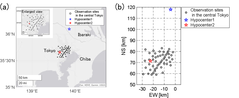
The observation sites assumed in the present paper are the subset of the observation sites of MeSO-net that actually exist in the central Tokyo of Japan. Figure 2 shows geometric settings. The circles indicate the assumed observation sites. The number of observation sites is 50. The origin of horizontal (NS-EW) coordinates is set as ($35.0340^{\circ}$N, $139.9106^{\circ}$E). Note that the results do not depend on the setting of the origin of horizontal coordinates since the relative positional relationship between the observation sites and the hypocenter affects the results.

The earthquake source is assumed to be located in the half-space as shown in Fig. 1. In the present paper, two types of earthquakes are simulated using different source information, and the characteristics of observation site selection by the proposed method are verified. The source information is set based on the earthquakes actually occurred in the Tokyo metropolitan area. Table 2 summarizes the source information. In the case of the hypocenter 1, the source information is set based on that of the earthquake which occurred in the southern part of Ibaraki prefecture on September 16, 2014. This area is known as one of areas where earthquakes occur frequently. In the case of the hypocenter 2, the source information is set based on that of the earthquake which occurred directly underneath the central Tokyo on May 9, 2010. The blue and red marks shown in Fig. 2 indicate the locations of the hypocenters 1 and 2. The cases of the hypocenters 1 and 2 correspond to situations where the earthquake occurs far from and directly underneath the area of observation sites, respectively.

In the present study, the seismic velocities of each of the three layers ($V_{Pi}$ and $V_{Si}$, where $i=1,2,3$) and the thickness ($h_{i}$) of each of the three layers, and source location in three directions ($S_{\mathrm{NS}}$, $S_{\mathrm{EW}}$, and $S_{\mathrm{UD}}$) are the estimation target of the model parameters following the previous studies (Kano et al., 2017a, b). Note that the origin time, which is estimated in the previous studies (Kano et al., 2017a, b), is not taken into account as a target parameter since Fourier spectra of the seismic wavefield is evaluated in the proposed method. The total number of model parameters to be estimated is $r=12$. The sensitivity matrix is constructed by simulating 24 cases using the code developed by Hisada (1995): 2 cases in which the value of one of the 12 parameters is changed by $+\Delta\phi$ and $-\Delta\phi$ from the initial value shown in Tables 1 and 2 are conducted, and then, the difference in Fourier spectra by $2\Delta\phi$ is obtained for each parameter. The values of $\Delta\phi$ for the subsurface structure model parameters ($V_{Pi}$, $V_{Si}$, and $h_{i}$) are set to $10\%$ of initial values (Table 1), and those for the source location parameters ($S_{\mathrm{NS}}$, $S_{\mathrm{EW}}$, and $S_{\mathrm{UD}}$) are set to 500 m.

The simulation was conducted in the frequency band from DC to 5 Hz. The number of frequency components is $i=205$. Hence, the number of components obtained by vector measurement at one observation site is $s=1230$ considering each frequency component consisting of the real and imaginary parts as shown in eq. 24. The second-order Butterworth filter was applied to the obtained simulation results in order to verify the influence of the frequency band of the seismic wavefield on the observation site selection. The lower cutoff frequency of the bandpass filter is set to be $0.1$ Hz, and the higher cutoff frequency varies from 0.3 Hz to 1.0 Hz at 0.1 Hz intervals.

In this subsection, normalized parameter sensitivity $\mathcal{S}$ is newly defined, and the characteristics of the parameter sensitivity matrix of interest in the proposed method are investigated. This is a scalar quantity showing the sensitivity of each observation site to each parameter.

We consider the difference in the observation data due to the difference in the $k$th parameter at the $j$th observation site. This corresponds to the numerator of $\tilde{\phi}_{k}\frac{\partial\mathbf{x}_{j}}{\partial\phi_{k}}$ in the normalized parameter sensitivity matrix in eq. (26). The difference in the observation data ($\Delta\mathbf{x}_{j}^{\phi_{k}}$) is expressed by the difference between the observation data in the case of $\phi_{k}=\phi_{k}+\Delta\phi_{k}$ and that in the case of $\phi_{k}=\phi_{k}-\Delta\phi_{k}$ as follows:

$$\Delta\mathbf{x}_{j}^{\phi_{k}}=\mathbf{x}_{j}|_{\phi_{k}=\phi_{k}+\Delta\phi_{k}}-\mathbf{x}_{j}|_{\phi_{k}=\phi_{k}-\Delta\phi_{k}}.$$

(31)

Here, $\Delta\phi$ in the present study was set to be the same value as that for constructing the normalized sensitivity matrix described in Section 3.1. Since the observation data $\mathbf{x}$ is a vector as shown in eq. (24), we define the sum of the squares of each component of the difference vector, that is, the square of the $L_{2}$ norm as the normalized parameter sensitivity to $k$th parameter of $j$th observation site ($\mathcal{S}_{j}^{\phi_{k}}$) as follows:

$$\mathcal{S}_{j}^{\phi_{k}}=||\Delta\mathbf{x}_{j}^{\phi_{k}}||^{2}_{2}.$$

(32)

The scalar value $\mathcal{S}_{j}^{\phi_{k}}$ can be evaluated for each observation $(j=1,\dots,50)$ and for each parameter $(k=1,\dots,12)$.

It should be noted that the quantity evaluated in the observation site selection is not exactly the same as $\mathcal{S}_{j}^{\phi_{k}}$. The proposed site selection method evaluates the value of sites based on the determinant of the normalized parameter sensitivity matrix which is the quantity showing the sensitivity of all considered parameters comprehensively.

In this subsection, the characteristics of observation site selection by the proposed method in the case of the hypocenter 1, and the frequency band of $0.1-1.0$ Hz is investigated in detail as a basic case in the present paper.

Figure 3 shows maps of the normalized parameter sensitivity of 12 parameters. The ranges of color bar in Fig. 3 were fixed for each physical parameter. The gray solid lines indicate concentric circles from the hypocenter location every 5 km. Figure 3 demonstrates that the normalized parameter sensitivity has a spatial structure and there are superiority and inferiority of sensitivity between layers or directions. Table 3 summarises the characteristics of the parameter sensitivity. The characteristics are discussed for each parameter below.

In this subsection, the effect of the frequency band of the seismic wavefield on the observation site selection is investigated. Figure 8 shows the results of observation site selection using the proposed method in the cases of different frequency bands. The higher cutoff frequency of the bandpass filter varies from 0.3 to 1.0 Hz in each figure plotted at from the top left to the bottom right in Fig. 8. Note that the result of the higher cutoff frequency of 1.0 Hz is the same as the result shown in Fig. 6. The comparison of the power spectral density of acceleration in the NS, EW, and UD directions is shown in Fig. 9. The power spectral density is sampled at the observation site with the shortest epicentral distance as an example. The results using the bandpass filter with the higher cutoff frequency of 0.3, 0.5, and 1.0 Hz are plotted together for comparison in Fig. 9. The comparison of the observation site selection in the cases of different frequency bands shown in Fig. 6 demonstrates that there is no effect of the frequency band on the observation site selection. Although the order of selection is slightly different depending on the frequency band, the comprehensive characteristics discussed in Section 3.3 is not affected by the frequency band. This is because the comprehensive characteristics of the seismic wavefield are the same between the cases of the different frequency bands. Figure 9 illustrates that the frequency spectra are quantitatively different depending on the frequency band; the values of the power spectral density at the dominant frequency increase significantly with increasing the higher cutoff frequency. However, the qualitative characteristics in the cases of 0.3, 0.5, and 1.0 Hz are the same as each other; the power spectral density is much higher in the NS direction than in the EW and UD directions, and the peak frequencies of the acceleration in the NS, EW, and UD directions does not change. In addition, maps of the normalized parameter sensitivity are confirmed not to be qualitatively affected by the frequency band. Therefore, the observation sites sensitive to the parameters are not considered to depend on the frequency band of the seismic wavefield.

In this subsection, the effect of the focal mechanisms on the observation site selection is discussed. The results in the case of the hypocenter 2 are compared to those in the case of the hypocenter 1 discussed in Section 3.3.

Figure 10 shows maps of the normalized parameter sensitivity of 12 parameters. The range of the color bar in Fig. 10 is set to be the same as each other for the same kind of physical parameters of different layers or directions. The gray lines indicate concentric circles from the hypocenter location. Table 5 summarises the effects of the focal mechanisms, and each parameter in the table is explained below.

Firstly, the characteristics of the sensitivity to seismic velocities $V_{P}$ and $V_{S}$ are discussed. Focusing on the magnitude relationship between layers, the sensitivity to $V_{P\rm{2}}$ and $V_{P\rm{3}}$ are much higher than that to $V_{P\rm{1}}$, and the sensitivity to $V_{S\rm{1}}$ and $V_{S\rm{2}}$ are much higher than that to $V_{S\rm{3}}$. These tendencies are similar to those of the case of the hypocenter 1 in Section 3.3.1; the magnitude relationship is due to the difference in the arrival time. Therefore, the magnitude relationship of the sensitivity to seismic velocities between layers does not depend on the focal mechanisms and is determined by the subsurface structure model parameters. Focusing on the spatial structure, the sensitivity to $V_{S}$ is high in the northern region adjacent to the hypocenter. The reason for the characteristics is consistent with the discussion on the case of the hypocenter 1 in Section 3.3.1; the spatial structure of the sensitivity to $V_{S}$ is due to the energy distribution of the S-wave. On the other hand, the characteristics of the spatial structure of the sensitivity to $V_{P}$ are different; although the sensitivity to $V_{P}$ is higher at observation sites with a larger epicentral distance in the case of the hypocenter 1, it is high in the north region and the southwest region in the case of the hypocenter 2. This is due to the energy distribution of the P-wave. Figure 11 shows the energy distribution in the UD direction obtained by calculating the sum of squares of the components in the UD direction of the frequency spectra. The energy distribution corresponds to that of the P-wave because the fluctuations in the NS and EW directions are dominant in the duration of the S-wave arrival and that in the UD direction is dominant in the duration of the P-wave arrival in the current case. The comparison of the energy distribution (Fig. 11) with the maps of sensitivity to $V_{P}$ (Fig. 10) demonstrates that the spatial structure of the sensitivity to $V_{P}$ is qualitatively the same as that of the energy distribution of the P-wave. Hence, the reason for the trend of the spatial structure is that the difference in the energy of the P-wave caused by the difference in $V_{P}$ increases with increasing originally the energy of the P-wave.

To summarize the discussions on the spatial structure of the sensitivity to $V_{P}$ above and in Section 3.3.1, the difference in the arrival time and the energy distribution of the P-wave are the dominant factors in the cases of the hypocenters 1 and 2, respectively. The discrepancy is mainly because the hypocenter is located approximately 30 to 50 km away from the observation site area in the case of the hypocenter 1, whereas in the case of the hypocenter 2, the hypocenter is directly below the observation site area, and the difference in the arrival time between the observation sites is relatively small. Therefore, factors that potentially affect the spatial structure of the sensitivity to seismic velocities do not depend on the focal mechanism; the difference in the arrival time and the energy distribution affects the sensitivity in both cases of hypocenter 1 and 2, but the dominant factor depends on the focal mechanism.

Secondly, the characteristics of the sensitivity to $h$ are discussed. The sensitivity to $h_{\rm 1}$ and $h_{\rm 2}$ is higher than that to $h_{\rm 3}$, and it is high in the northern region adjacent to the hypocenter. The reasons for these characteristics are consistent with the discussions on the case of the hypocenter 1 in Section 3.3.2; the characteristics of the sensitivity to $h$ are determined by those to $V_{P}$ and $V_{S}$. Therefore, factors that affect the characteristics of the sensitivity to $h$ do not depend on the focal mechanisms.

Finally, the characteristics of the sensitivity to $S_{\mathrm{NS}}$, $S_{\mathrm{EW}}$, and $S_{\mathrm{UD}}$ are discussed. The sensitivity to $S_{\mathrm{UD}}$ is much higher than that of $S_{\mathrm{NS}}$ and $S_{\mathrm{EW}}$, and $S_{\mathrm{UD}}$ is higher in the northern region adjacent to the hypocenter. The reasons for these characteristics are consistent with the discussions on the case of the hypocenter 1 in Section 3.3.3; the characteristics of the sensitivity to the hypocenter locations are characterized by the positional relationship and the energy distribution of the S-wave. Therefore, factors that potentially affect the characteristics of the sensitivity to hypocenter locations do not depend on the focal mechanism.

Figure 12 shows the result of observation site selection using the proposed method in the case of the hypocenter 2 and the frequency band of $0.1$–1.0 Hz. The observation sites are colored from red to blue depending on the order of selection. Figure 13 shows the normalized parameter sensitivity against observation sites in the order of selection. Figure 12 indicates that observation sites in the northern region adjacent to the hypocenter are preferentially selected by the proposed method. This trend is due to the characteristics of the normalized parameter sensitivity discussed above; Fig. 13 demonstrates that the values of sensitivity decrease comprehensively as the selection order of observation sites decreases. Especially in the case of the hypocenter 2, the sensitivity to $V_{S}$, $h$, and $S_{\mathrm{UD}}$ decreases with the selection order, whereas there is no correlation between the selection order and other parameters such as $V_{P}$, $S_{\mathrm{NS}}$, and $S_{\mathrm{EW}}$. This is mainly because the spatial structure of the sensitivity to $V_{S}$, $h$, and $S_{\mathrm{UD}}$ is major among all parameters, whereas those of other parameters are different from the major one. Therefore, the proposed method is confirmed to be able to select observation sites suitable for improvement of the average sensitivity to all parameters according to the sensitivity characteristics, which depends on the focal mechanism.

The seismic velocities ($V_{p}$ and $V_{s}$) and the thickness ($h$) of each of the three layers, and source location in three directions ($S_{\mathrm{NS}}$, $S_{\mathrm{EW}}$, and $S_{\mathrm{UD}}$) are employed as the target model parameters to be estimated as with Section 3. The observation sites are the same as that in Section 3.1. Hence, the initial values of the subsurface structure model parameters are based on Koketsu et al. (2011) summarized in Table 1. The earthquake source information is the same as the case of the hypocenter 1 in Section 3, and the initial values of the source parameters are summarized in Table 2. True values of the 12 model parameters are assumed to be slightly different from the initial values in the numerical experiment. The true values are obtained by adding the small values to the initial values. The small value is obtained by multiplying the random value following a normal distribution $\mathcal{N}(0,1)$ by $10\%$ of the initial value and 5 km for subsurface structure model parameters and source location parameters, respectively. The reconstruction of waveforms within a frequency band of 0.1–1.0 Hz is examined in the present experiment. Thus, the simulation was conducted in the frequency range less 5 Hz as with Section 3.1, and the second-order Butterworth filter of the frequency band of 0.1–1.0 Hz was applied to the obtained simulation results. The observation noise is added to the observation data $\mathbf{y}_{p}$ calculated using the code developed by Hisada (1995) in the frequency domain; the amplitude of additive noise for each component of observed data (each entry of $\mathbf{y}_{p}$) follows a normal distribution $\mathcal{N}(0,10^{-5})$. Figure 14 shows the power spectral density in the NS, EW, and UD directions of the true and additive noise signals. The true signals are obtained by the simulation using the true model parameters. Three observation sites out of 50 candidates are used for the parameter estimation. Hence, the observation sites numbered 1, 2, and 3 in Fig. 6 are employed in the proposed method. The experiments using 100 patterns of subsets of three randomly selected observation sites are conducted for comparison. Note that the results of the comparison between the proposed method and averaged results with random selection in the case of three observation sites are qualitatively the same regardless of the number of observation sites, and the superiority of the proposed method tends to increase as the number of observation sites decreases.

The relation between the reconstruction error of the seismic wavefield and the iteration number of estimation [eq. (28)–(30)] is described in Fig. 15 in the case of three observation sites used for the model parameter estimation. The reconstruction error of the seismic wavefield was calculated as follows:

$\displaystyle\epsilon=\frac{||\mathbf{X}^{\rm true}-\mathbf{X}^{\rm reconst}||_{\rm F}}{||\mathbf{X}^{\rm true}||_{\rm F}},$

(33)

where the notation $\|\circ\|_{\mathrm{F}}$ is the Frobenius norm that is the matrix norm as the square root of the sum of the absolute squares of the matrix elements. The matrix $\mathbf{X}^{\rm true}$ is the true data calculated using the true model parameters, and $\mathbf{X}^{\rm reconst}$ is the reconstructed data using the estimated model parameters based on the observed signals at three observation sites. The values of the random selection shown in Fig. 15 are an average over the results using 100 patterns of subsets of three randomly selected observation sites. Figure 16 shows the reconstruction error distributions of the seismic wavefields using three observation sites selected by the proposed method and using three randomly selected observation sites, respectively. The reconstruction error presented in Fig. 16 is evaluated at each observation site when the number of iterations $t$ is 20. The values for case of the random selection are the result using one pattern of subsets of three randomly selected observation sites in Fig. 16. The observation sites selected using the proposed method and those randomly selected are numbered and marked with an asterisk in Fig. 16, respectively. Figure 17 shows the power spectral density of seismic acceleration in the NS, EW, and UD directions at two observation sites, excluding the selected observation sites by the proposed method and those randomly selected in semilog plots. The two observation sites are marked by (a) and (b) in Fig. 16, which correspond to the observation site near the center of the observation area and the one with the longest epicentral distance, respectively.

Figure 15 indicates that although the reconstruction error decreases as the number of iterations for optimisation of the model parameter estimation increases both in the results using the observation sites selected by the proposed method and in the results using the randomly selected observation sites, the reconstruction error can be minimized by the proposed method. In addition, Fig. 16 demonstrates that in the result using the randomly selected observation sites, although the reconstruction error is relatively small at and around the three selected observation sites, the reconstruction error is significant at the sites away from the three sites. On the other hand, the estimation using the proposed method can reduce the reconstruction error compared to that using the randomly selected observation sites at almost all observation sites. Figure 17 indicates that the PSD reconstructed with the parameters estimated using the observation sites selected by the proposed method matches the true values more accurately than that using the randomly selected observation sites, although the difference between the PSD reconstructed using the proposed method and that using random selection is unfortunately invisible in this range. Although these small differences are due to the assumption in the present experiment which gives the quite small discrepancies between the initial and true values of the model parameters in the present study, the estimation is somehow improved in this small range by using optimised sensor locations as previously shown in Fig. 15. The small but certain improvement in the estimation shows the selected locations are sensitive to the parameters of the model. The sensitive sensor location is expected to be also applicable to the parameter search in the practical nonlinear problem, which is left for the future study.

Figure 18 shows the relation between the estimation error of each model parameter and the iteration number of estimation (eq. (28)–(30)), where the estimation error of the model parameter was defined as the relative error between the estimated value and the true value. Although the estimation error converges to a constant value as the number of iterations increases both in the results using the observation sites selected by the proposed method and in the results using the randomly selected observation sites, the proposed method can reduce the estimation error of almost all parameters compared to that using the random selection. These results confirm that the optimised observation sites using the proposed method can reconstruct the seismic wavefield with high accuracy by estimating the model parameters accurately as expected. Note that the small differences are due to the assumption in the present experiment which gives the quite small discrepancies between the initial and true values of the model parameters in the present study as stated above.

The relationship between the number of observation sites and the reconstruction error is described in Fig.19. Figure 19 demonstrates that the reconstruction error tends to decrease as the number of observation sites increases. The reconstruction error with the parameters estimated using the observation sites selected by the proposed methods asymptotically approaches a small value when more than three observation sites are used. On the other hand, the error using the random selection becomes as small as that using the proposed method when 15 or more observation sites are used. Therefore, the superiority of the proposed method is remarkable for the reconstruction using 10 or less observation sites in the numerical experiments of the present study. However, with regard to the reconstruction using only one or two observation sites, the reconstruction error using the selected observation sites by the proposed method is within the error bars of that using the randomly selected observation sites. This is because the proposed method first selects an observation site that contributes the most to the minimization of the determinant of the normalized parameter sensitivity matrix as described in eq. (23), and the strategy is not exactly consistent with selecting one that most reduces the reconstruction error of the seismic wavefield. On the other hand, as the number of observation sites increases, the proposed method can select a subset of observation sites suitable for accurate estimation for almost all parameters, since the determinant represents the average sensitivity of all parameters. Therefore, the superiority of the proposed method emerges when the number of observation sites is relatively small, within the range formulated in the combinatorial optimisation problem. The condition is between three and ten observation sites in the numerical experiments of the present study.

References

- Aoi & Fujiwara (1999) Aoi, S. & Fujiwara, H., 1999. 3d finite-difference method using discontinuous grids, Bulletin of the Seismological Society of America, 89(4), 918–930.
- Arnold & Curtis (2018) Arnold, R. & Curtis, A., 2018. Interrogation theory, Geophysical Journal International, 214(3), 1830–1846.
- Atkinson et al. (2007) Atkinson, A., Donev, A., Tobias, R., et al., 2007. Optimum experimental designs, with SAS, vol. 34, Oxford University Press.
- Boore (1972) Boore, D. M., 1972. Finite difference methods for seismic wave propagation in heterogeneous materials, Methods in computational physics, 11, 1–37.
- Callaham et al. (2019) Callaham, J. L., Maeda, K., & Brunton, S. L., 2019. Robust flow reconstruction from limited measurements via sparse representation, Physical Review Fluids, 4(10), 103907.
- Carter et al. (2021) Carter, D. W., De Voogt, F., Soares, R., & Ganapathisubramani, B., 2021. Data-driven sparse reconstruction of flow over a stalled aerofoil using experimental data, Data-Centric Engineering, 2.
- Chaloner & Verdinelli (1995) Chaloner, K. & Verdinelli, I., 1995. Bayesian experimental design: A review, Statistical Science, 10(3), 273–304.
- Clark et al. (2018) Clark, E., Askham, T., Brunton, S. L., & Kutz, J. N., 2018. Greedy sensor placement with cost constraints, IEEE Sensors Journal, 19(7), 2642–2656.
- Clark et al. (2020a) Clark, E., Brunton, S. L., & Kutz, J. N., 2020a. Multi-fidelity sensor selection: Greedy algorithms to place cheap and expensive sensors with cost constraints, IEEE Sensors Journal, 21(1), 600–611.
- Clark et al. (2020b) Clark, E., Kutz, J. N., & Brunton, S. L., 2020b. Sensor selection with cost constraints for dynamically relevant bases, IEEE Sensors Journal, 20(19), 11674–11687.
- Du et al. (2014) Du, W., Xing, Z., Li, M., He, B., Chua, L. H. C., & Miao, H., 2014. Optimal sensor placement and measurement of wind for water quality studies in urban reservoirs, in IPSN-14 Proceedings of the 13th International Symposium on Information Processing in Sensor Networks, pp. 167–178, IEEE.
- Earl & Deem (2005) Earl, D. J. & Deem, M. W., 2005. Parallel tempering: Theory, applications, and new perspectives, Physical Chemistry Chemical Physics, 7(23), 3910–3916.
- Fujita et al. (2014) Fujita, K., Ichimura, T., Hori, M., Wijerathne, M., & Tanaka, S., 2014. A quick earthquake disaster estimation system with fast urban earthquake simulation and interactive visualization, Procedia Computer Science, 29, 866–876.
- Fukami et al. (2021) Fukami, K., Maulik, R., Ramachandra, N., Fukagata, K., & Taira, K., 2021. Global field reconstruction from sparse sensors with voronoi tessellation-assisted deep learning, Nature Machine Intelligence, 3(11), 945–951.
- Geyer (1991) Geyer, C. J., 1991. Markov chain monte carlo maximum likelihood.
- Hardt & Scherbaum (1994) Hardt, M. & Scherbaum, F., 1994. The design of optimum networks for aftershock recordings, Geophysical Journal International, 117(3), 716–726.
- Hirata (2009) Hirata, N., 2009. An outline of the special project for earthquake disaster mitigation in the tokyo metropolitan area-subproject i: characterization of the plate structure and source faults in and around the tokyo metropolitan area, Bull. Earthq. Res. Inst. Univ. Tokyo, 84, 41–56.
- Hisada (1995) Hisada, Y., 1995. An efficient method for computing green’s functions for a layered half-space with sources and receivers at close depths (part 2), Bulletin of the Seismological Society of America, 85(4), 1080–1093.
- Hisada & Bielak (2003) Hisada, Y. & Bielak, J., 2003. A theoretical method for computing near-fault ground motions in layered half-spaces considering static offset due to surface faulting, with a physical interpretation of fling step and rupture directivity, Bulletin of the Seismological Society of America, 93(3), 1154–1168.
- Hukushima & Nemoto (1996) Hukushima, K. & Nemoto, K., 1996. Exchange monte carlo method and application to spin glass simulations, Journal of the Physical Society of Japan, 65(6), 1604–1608.
- Ichimura et al. (2007) Ichimura, T., Hori, M., & Kuwamoto, H., 2007. Earthquake motion simulation with multiscale finite-element analysis on hybrid grid, Bulletin of the Seismological Society of America, 97(4), 1133–1143.
- Inoba et al. (2022) Inoba, R., Uchida, K., Iwasaki, Y., Nagata, T., Ozawa, Y., Saito, Y., Nonomura, T., & Asai, K., 2022. Optimization of sparse sensor placement for estimation of wind direction and surface pressure distribution using time-averaged pressure-sensitive paint data on automobile model, Journal of Wind Engineering and Industrial Aerodynamics, 227, 105043.
- Inoue et al. (2021) Inoue, T., Matsuda, Y., Ikami, T., Nonomura, T., Egami, Y., & Nagai, H., 2021. Data-driven approach for noise reduction in pressure-sensitive paint data based on modal expansion and time-series data at optimally placed points, Physics of Fluids, 33(7), 077105.
- Inoue et al. (2023) Inoue, T., Ikami, T., Egami, Y., Nagai, H., Naganuma, Y., Kimura, K., & Matsuda, Y., 2023. Data-driven optimal sensor placement for high-dimensional system using annealing machine, Mechanical Systems and Signal Processing, 188, 109957.
- Joshi & Boyd (2009) Joshi, S. & Boyd, S., 2009. Sensor selection via convex optimization, IEEE Transactions on Signal Processing, 57(2), 451–462.
- Kameda & Morikawa (1992) Kameda, H. & Morikawa, H., 1992. An interpolating stochastic process for simulation of conditional random fields, Probabilistic Engineering Mechanics, 7(4), 243–254.
- Kameda & Morikawa (1994) Kameda, H. & Morikawa, H., 1994. Conditioned stochastic processes for conditional random fields, Journal of engineering mechanics, 120(4), 855–875.
- Kanda et al. (2021) Kanda, N., Nakai, K., Saito, Y., Nonomura, T., & Asai, K., 2021. Feasibility study on real-time observation of flow velocity field using sparse processing particle image velocimetry, Transactions of the Japan Society for Aeronautical and Space Sciences, 64(4), 242–245.
- Kanda et al. (2022) Kanda, N., Abe, C., Goto, S., Yamada, K., Nakai, K., Saito, Y., Asai, K., & Nonomura, T., 2022. Proof-of-concept study of sparse processing particle image velocimetry for real time flow observation, Experiments in Fluids, 63(9), 143.
- Kaneko et al. (2021) Kaneko, S., Ozawa, Y., Nakai, K., Saito, Y., Nonomura, T., Asai, K., & Ura, H., 2021. Data-driven sparse sampling for reconstruction of acoustic-wave characteristics used in aeroacoustic beamforming, Applied Sciences, 11(9), 4216.
- Kano et al. (2017a) Kano, M., Nagao, H., Ishikawa, D., Ito, S.-i., Sakai, S., Nakagawa, S., Hori, M., & Hirata, N., 2017a. Seismic wavefield imaging based on the replica exchange monte carlo method, Geophysical Journal International, 208(1), 529–545.
- Kano et al. (2017b) Kano, M., Nagao, H., Nagata, K., Ito, S.-i., Sakai, S., Nakagawa, S., Hori, M., & Hirata, N., 2017b. Seismic wavefield imaging of long-period ground motion in the tokyo metropolitan area, japan, Journal of Geophysical Research: Solid Earth, 122(7), 5435–5451.
- Kawakami (1989) Kawakami, H., 1989. Simulation of space-time variation of earthquake ground motion including a recorded time history, Doboku Gakkai Ronbunshu, 1989(410), 435–443.
- Kihara & Okada (1984) Kihara, M. & Okada, T., 1984. A satellite selection method and accuracy for the global positioning system, Navigation, 31(1), 8–20.
- Kirkpatrick et al. (1983) Kirkpatrick, S., Gelatt Jr, C. D., & Vecchi, M. P., 1983. Optimization by simulated annealing, science, 220(4598), 671–680.
- Koketsu et al. (2004) Koketsu, K., Fujiwara, H., & Ikegami, Y., 2004. Finite-element simulation of seismic ground motion with a voxel mesh, Pure and Applied Geophysics, 161(11-12).
- Koketsu et al. (2011) Koketsu, K., Yokota, Y., Nishimura, N., Yagi, Y., Miyazaki, S., Satake, K., Fujii, Y., Miyake, H., Sakai, S., Yamanaka, Y., et al., 2011. A unified source model for the 2011 tohoku earthquake, Earth and Planetary Science Letters, 310(3-4), 480–487.
- Kraft et al. (2013) Kraft, T., Mignan, A., & Giardini, D., 2013. Optimization of a large-scale microseismic monitoring network in northern switzerland, Geophysical Journal International, 195(1), 474–490.
- Langston (2007a) Langston, C. A., 2007a. Spatial gradient analysis for linear seismic arrays, Bulletin of the Seismological Society of America, 97(1B), 265–280.
- Langston (2007b) Langston, C. A., 2007b. Wave gradiometry in two dimensions, Bulletin of the Seismological Society of America, 97(2), 401–416.
- Li et al. (2021a) Li, B., Liu, H., & Wang, R., 2021a. Data-driven sensor placement for efficient thermal field reconstruction, Science China Technological Sciences, 64(9), 1981–1994.
- Li et al. (2021b) Li, B., Liu, H., & Wang, R., 2021b. Efficient sensor placement for signal reconstruction based on recursive methods, IEEE Transactions on Signal Processing, 69, 1885–1898.
- Liang & Langston (2009) Liang, C. & Langston, C. A., 2009. Wave gradiometry for usarray: Rayleigh waves, Journal of Geophysical Research: Solid Earth, 114(B2).
- Liu et al. (2016) Liu, S., Chepuri, S. P., Fardad, M., Maşazade, E., Leus, G., & Varshney, P. K., 2016. Sensor selection for estimation with correlated measurement noise, IEEE Transactions on Signal Processing, 64(13), 3509–3522.
- Long et al. (2015) Long, Q., Motamed, M., & Tempone, R., 2015. Fast bayesian optimal experimental design for seismic source inversion, Computer Methods in Applied Mechanics and Engineering, 291, 123–145.
- Maeda et al. (2016) Maeda, T., Nishida, K., Takagi, R., & Obara, K., 2016. Reconstruction of a 2d seismic wavefield by seismic gradiometry, Progress in Earth and Planetary Science, 3(1), 1–17.
- Manohar et al. (2018) Manohar, K., Brunton, B. W., Kutz, J. N., & Brunton, S. L., 2018. Data-driven sparse sensor placement for reconstruction: Demonstrating the benefits of exploiting known patterns, IEEE Control Systems Magazine, 38(3), 63–86.
- Manohar et al. (2019) Manohar, K., Kaiser, E., Brunton, S. L., & Kutz, J. N., 2019. Optimized sampling for multiscale dynamics, Multiscale Modeling & Simulation, 17(1), 117–136.
- Manohar et al. (2021) Manohar, K., Kutz, J. N., & Brunton, S. L., 2021. Optimal sensor and actuator selection using balanced model reduction, IEEE Transactions on Automatic Control, 67(4), 2108–2115.
- Muir & Zhan (2021) Muir, J. B. & Zhan, Z., 2021. Seismic wavefield reconstruction using a pre-conditioned wavelet–curvelet compressive sensing approach, Geophysical Journal International, 227(1), 303–315.
- Muir & Zhan (2022) Muir, J. B. & Zhan, Z., 2022. Wavefield-based evaluation of das instrument response and array design, Geophysical Journal International, 229(1), 21–34.
- Nagata et al. (2021) Nagata, T., Nonomura, T., Nakai, K., Yamada, K., Saito, Y., & Ono, S., 2021. Data-driven sparse sensor selection based on a-optimal design of experiment with admm, IEEE Sensors Journal, 21(13), 15248–15257.
- Nagata et al. (2022a) Nagata, T., Nakai, K., Yamada, K., Saito, Y., Nonomura, T., Kano, M., Ito, S.-i., & Nagao, H., 2022a. Seismic wavefield reconstruction based on compressed sensing using data-driven reduced-order model, Geophysical Journal International, 322(1), 33–50.
- Nagata et al. (2022b) Nagata, T., Yamada, K., Nonomura, T., Nakai, K., Saito, Y., & Ono, S., 2022b. Data-driven sensor selection method based on proximal optimization for high-dimensional data with correlated measurement noise, IEEE Transactions on Signal Processing, pp. 5251–5264.
- Nagata et al. (2023) Nagata, T., Yamada, K., Nakai, K., Saito, Y., & Nonomura, T., 2023. Randomized group-greedy method for large-scale sensor selection problems, IEEE Sensors Journal.
- Nakai et al. (2021) Nakai, K., Yamada, K., Nagata, T., Saito, Y., & Nonomura, T., 2021. Effect of objective function on data-driven greedy sparse sensor optimization, IEEE Access, 9, 46731–46743.
- Nakai et al. (2022) Nakai, K., Sasaki, Y., Nagata, T., Yamada, K., Saito, Y., & Nonomura, T., 2022. Nondominated-solution-based multi-objective greedy sensor selection for optimal design of experiments, IEEE Transactions on Signal Processing, 70, 5694–5707.
- Nonomura et al. (2021) Nonomura, T., Ono, S., Nakai, K., & Saito, Y., 2021. Randomized subspace newton convex method applied to data-driven sensor selection problem, IEEE Signal Processing Letters, 28, 284–288.
- Phatak (2001) Phatak, M. S., 2001. Recursive method for optimum gps satellite selection, IEEE Transactions on Aerospace and Electronic Systems, 37(2), 751–754.
- Pitarka (1999) Pitarka, A., 1999. 3d elastic finite-difference modeling of seismic motion using staggered grids with nonuniform spacing, Bulletin of the Seismological Society of America, 89(1), 54–68.
- Saito et al. (2020) Saito, Y., Nonomura, T., Nankai, K., Yamada, K., Asai, K., Sasaki, Y., & Tsubakino, D., 2020. Data-driven vector-measurement-sensor selection based on greedy algorithm, IEEE Sensors Letters, 4.
- Saito et al. (2021a) Saito, Y., Nonomura, T., Yamada, K., Nakai, K., Nagata, T., Asai, K., Sasaki, Y., & Tsubakino, D., 2021a. Determinant-based fast greedy sensor selection algorithm, IEEE Access, 9, 68535–68551.
- Saito et al. (2021b) Saito, Y., Yamada, K., Kanda, N., Nakai, K., Nagata, T., Nonomura, T., & Asai, K., 2021b. Data-driven determinant-based greedy under/oversampling vector sensor placement, CMES-COMPUTER MODELING IN ENGINEERING & SCIENCES, 129(1), 1–30.
- Sakai & Hirata (2009) Sakai, S. & Hirata, N., 2009. Distribution of the metropolitan seismic observation network, Bull. Earthq. Res. Inst. Univ. Tokyo, 84, 57–69.
- Sato & Imabayashi (1999) Sato, T. & Imabayashi, H., 1999. Real time conditional simulation of earthquake ground motion, Earthquake Engineering and Engineering Seismology, 1(1), 27–38.
- Schneider et al. (2018) Schneider, S., Thomas, C., Dokht, R. M., Gu, Y. J., & Chen, Y., 2018. Improvement of coda phase detectability and reconstruction of global seismic data using frequency–wavenumber methods, Geophysical Journal International, 212(2), 1288–1301.
- Shamaiah et al. (2010) Shamaiah, M., Banerjee, S., & Vikalo, H., 2010. Greedy sensor selection: Leveraging submodularity, in 49th IEEE conference on decision and control (CDC), pp. 2572–2577, IEEE.
- Shiina et al. (2021) Shiina, T., Maeda, T., Kano, M., Kato, A., & Hirata, N., 2021. An optimum 2d seismic-wavefield reconstruction in densely and nonuniformly distributed stations: The metropolitan seismic observation network in japan, Seismological Society of America, 92(3), 2015–2027.
- Steinberg & Rabinowitz (2003) Steinberg, D. M. & Rabinowitz, N., 2003. Optimal seismic monitoring for event location with application to on site inspection of the comprehensive nuclear test ban treaty, Metrika, 58(1), 31–57.
- Stuart (2010) Stuart, A. M., 2010. Inverse problems: A bayesian perspective, Acta Numerica, 19, 451–559.
- Swendsen & Wang (1986) Swendsen, R. H. & Wang, J.-S., 1986. Replica monte carlo simulation of spin-glasses.
- Tiwari et al. (2022) Tiwari, N., Uchida, K., Inoba, R., Saito, Y., Asai, K., & Nonomura, T., 2022. Simultaneous measurement of pressure and temperature on the same surface by sensitive paints using the sensor selection method, Experiments in Fluids, 63(11), 1–13.
- Uciński (2020) Uciński, D., 2020. D-optimal sensor selection in the presence of correlated measurement noise, Measurement, 164, 107873.
- Vanmarcke & Fenton (1991) Vanmarcke, E. H. & Fenton, G. A., 1991. Conditioned simulation of local fields of earthquake ground motion, Structural Safety, 10(1-3), 247–264.
- Wald et al. (1999) Wald, D. J., Quitoriano, V., Heaton, T. H., Kanamori, H., Scrivner, C. W., & Worden, C. B., 1999. Trinet “shakemaps”: Rapid generation of peak ground motion and intensity maps for earthquakes in southern california, Earthquake Spectra, 15(3), 537–555.
- Wald et al. (2005) Wald, D. J., Worden, B. C., Quitoriano, V., & Pankow, K. L., 2005. Shakemap manual: technical manual, user’s guide, and software guide, Tech. rep.
- Worden & Burrows (2001) Worden, K. & Burrows, A., 2001. Optimal sensor placement for fault detection, Engineering structures, 23(8), 885–901.
- Yamada et al. (2021) Yamada, K., Saito, Y., Nankai, K., Nonomura, T., Asai, K., & Tsubakino, D., 2021. Fast greedy optimization of sensor selection in measurement with correlated noise, Mechanical Systems and Signal Processing, 158, 107619.
- Yamada et al. (2022) Yamada, K., Saito, Y., Nonomura, T., & Asai, K., 2022. Greedy sensor selection for weighted linear least squares estimation under correlated noise, IEEE Access, 10, 79356–79364.
- Yeo et al. (2022) Yeo, W.-J., Taulu, S., & Kutz, J. N., 2022. Efficient magnetometer sensor array selection for signal reconstruction and brain source localization, arXiv preprint arXiv:2205.10925.
- Yi et al. (2011) Yi, T.-H., Li, H.-N., & Gu, M., 2011. Optimal sensor placement for structural health monitoring based on multiple optimization strategies, The Structural Design of Tall and Special Buildings, 20(7), 881–900.
- Zhan et al. (2018) Zhan, Z., Li, Q., & Huang, J., 2018. Application of wavefield compressive sensing in surface wave tomography, Geophysical Journal International, 213(3), 1731–1743.
- Zhang & Curtis (2021) Zhang, X. & Curtis, A., 2021. Interrogating probabilistic inversion results for subsurface structural information, Geophysical Journal International, 229(2), 750–757.
- Zhao et al. (2022) Zhao, X., Curtis, A., & Zhang, X., 2022. Interrogating subsurface structures using probabilistic tomography: An example assessing the volume of irish sea basins, Journal of Geophysical Research: Solid Earth, 127(4), e2022JB024098.