Observation of the Knot Topology of Non-Hermitian Systems in a Single Spin
Abstract
The non-Hermiticity of the system gives rise to distinct knot topology that has no Hermitian counterpart.
Here, we report a comprehensive study of the knot topology in gapped non-Hermitian systems based on the universal dilation method with a long coherence time nitrogen-vacancy center in a C isotope purified diamond.
Both the braiding patterns of energy bands and the eigenstate topology are revealed.
Furthermore, the global biorthogonal Berry phase related to the eigenstate topology has been successfully observed, which identifies the topological invariance for the non-Hermitian system.
Our method paves the way for further exploration of the interplay among band braiding, eigenstate topology and symmetries in non-Hermitian quantum systems.
The non-Hermitian (NH) Hamiltonian has drawn intensive attention RMP_Bergholtz ; PRL_NHtopo1 ; PRX_NHtopo1 ; PRX_NHtopo2 ; Science_NHtopo ; PRL_NHtopo2 ; PRA_NHtopo due to its application in photonic Science_NHApli1 ; NP_NHApli ; Science_NHApli2 ; Science_NHApli3 ; Nature_PhotoNH ; Science_PhotoNH1 ; PRL_PhotoNH1 ; PRL_PhotoNH2 ; PRL_PhotoNH3 ; NaturePhotonics_PhotoNH ; NP_PhotoNH and acoustic NHAcous_Romain ; NHAcous_Tuo ; NHAcous_Zhi systems with gain and loss, open quantum systems JPA_OpenNH ; Nature_OpenNH ; PRL_OpenNHCar ; NP_OpenNHDiehl and condensed matter systems of quasi-particles with finite lifetime Arxiv_CondNH ; PRB_CondNH1 ; PRB_CondNH2 ; PRL_CondNH . In contrast to Hermitian systems, topological structures that are exclusive to NH systems give birth to many intriguing phenomena like NH bulk boundary correspondence PRL_Kai ; PRL_Dan and NH skin effects PRL_Nobuyuki . The emergence of NH nodal phases and gapped phases as well as their interplay with symmetry also adds new ingredients for NH topological band theory RMP_Bergholtz . Understanding the topology introduced by NH physics helps one to explore topologically robust quantities and non-trivial edge states. All these uncommon phenomena provide insights into NH systems.
More recently, researchers have found a framework based on homotopy theory PRB_Fan ; PRL_Haiping ; PRB_ZhiLi to classify the non-Hermitian topological phases. Compared with the K-theory PRX_NHtopo1 , this classification method does not need to assume specific symmetries and can reveal more topological invariants. To be precise, the Hamiltonian can be regarded as a mapping from the Brillouin zone to the space of energy bands and eigenstates. Thus the classification is done by finding all topologically non-equivalent mappings. Each class of mapping corresponds to a topological phase with a specific topological invariant. The non-Hermiticity of the Hamiltonian can generate complex eigenvalues, which can constitute the knot structures. The whole classification set of NH systems with knot topology is decomposed into several sectors, based on the braiding of eigenvalues, and each sector can be further classified with the eigenstate topology PRB_ZhiLi .
There are several experimental studies recently aiming at revealing the knot topology of the NH systems. For example, the braiding structure of energy bands has been observed in optical Nature_Fan , mechanical Nature_Harris and trapped ion PRL_Cao systems. A comprehensive demonstration of the knot topology, especially the essential information from the eigenstate topology requires coherent evolution under the NH Hamiltonian. It is difficult to realize NH Hamiltonians in quantum systems since closed systems are generally governed by Hermitian Hamiltonians. Apart from the difficulty in realizing a NH Hamiltonian, the inevitable decoherence of the quantum system tends to destroy the coherent evolution. In order to overcome these difficulties, we applied the universal dilation method Science_YW ; PRL_Wengang ; PRL_Uwe ; PRL_Kohei to realize the NH Hamiltonians and fabricated a 99.999% C isotope purified sample in which the decoherence had been significantly suppressed. Taking the one-dimensional (1D) NH lattice model as an example, we experimentally studied the knot topology in the NH Hamiltonian by measuring not only its energy eigenvalues, but also the corresponding eigenstates to reveal the global Berry phase. Compared with the NH topology shown in previous work PRL_Wengang on the NV center, which stems from encircling varying numbers of exceptional points, the knot topology investigated in our work arises from both the braiding of all energy bands and the eigenstate topology. Our platform is capable of dealing with other models and our results shed light on the complexity of topological features aroused by non-Hermiticity.
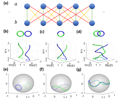
Here we consider a two-band NH 1D lattice model (Fig. 1(a)) whose Hamiltonian may be written as
| (1) |
where is the annihilation operator of sublattice on the th site, and the ’s are complex numbers representing the coupling strengths, i.e., is the on-site interaction and is the hopping between sublattice at site and lattice at site . Under the periodic boundary condition, the corresponding momentum space Hamiltonian is
| (2) | ||||
This model holds plenty of topological phases under different parameter configurations that ensure bands being separable. For , i.e., the nearest coupling case, the system may be in the unlink phase or the unknot phase. Because and are equivalent due to the periodic condition, the energy bands form closed curves. When the parameters are set as and , the non-Hermitian system is in the unlink phase, where the two circles are unrelated, as shown by Fig. 1(b). If the parameters are changed to and , the system will be in the unknot phase. There is only one circle because the two bands exchange (Fig. 1(c)). For , the next nearest coupling enriches the topological phases in addition to the unlink and unknot. When the parameters are set as and , the two eigenvalues form a non-trivial braiding structure. The energy bands braid around each other exactly once and this gives the Hopf link phase (Fig. 1(d)). The eigenstates also exhibit behaviors similar to those of the corresponding energy bands as shown in Fig. 1(e), 1(f) and 1(g). For larger , the energy bands may braid more times, which leads to more phases. The classification based on homotopy theory has shown that all phases of this model are described by the braiding group PRB_Fan ; PRB_ZhiLi .
We now study the topological phases of our model and the corresponding topological invariants in a quantum system based on the eigenvalues and eigenstates. Both the eigenvalues and the eigenstates can be obtained from the evolution under the NH Hamiltonian . Let (the dependence is omitted for simplicity in the following) be the eigenstates with complex eigenvalues , where and are real and imaginary parts of , respectively. For any initial state written as , the evolution governed by gives . Without loss of generality, we assume . The eigenvalues can be extracted from the time evolution of the populations of , and the steady state of NH evolution will be the eigenstate since is larger than . By implementing evolution governed by , the eigenstate can be obtained, which is due to for .
The evolution under the NH Hamiltonian can be realized based on the universal dilation method. The state of the system needs to evolve as . By introducing an ancilla, the NH evolution can be realized in a subspace while the total Hamiltonian is Hermitian. The initial state that reads evolves to under the Hamiltonian , where are eigenstates of and is a properly chosen time-dependent operator. Thus in the subspace, apart from a normalization constant, the evolution is strictly governed by .
We use a single nitrogen-vacancy (NV) center in diamond to experimentally realize the momentum space NH Hamiltonian for different phases with (see Appendix A for details of the experimental setup). The NV center is a type of point defect in diamond that is composed of a nitrogen atom and a neighbor vacancy as shown in Fig. 2(a). The ground-state of the NV center is a triplet state with an electronic spin that interacts with the nuclear spin of the substitutional N. We construct the dilated Hamiltonian in the subspace spanned by the states , and as shown in Fig. 2(b). The energy levels are relabeled as , and , respectively. The electron spin is chosen to be the system and nuclear spin serves as the ancilla.
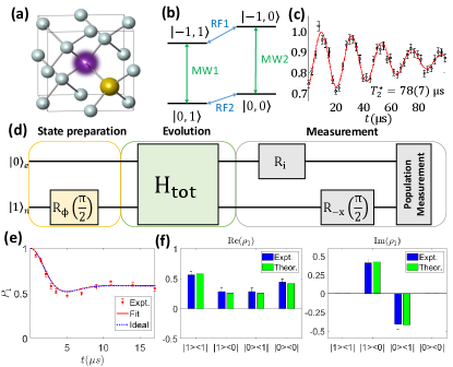
The pulse sequence used to realize the evolution under the NH Hamiltonian is shown in Fig. 2(d). The external static magnetic field was set to be 506 G. The state of the NV center was polarized to by 532-nm laser pulses Polarization . After polarization, the initial state is prepared by the RF pulse , where the rotation axis lies in the XY plane and atan is the angle between the rotation axis and the axis. Here we have chosen . The evolution under is realized by applying two selective microwave (MW) pulses, and the coherent evolution should be long enough to drive the system to a steady state. To this end, is multiplied by an overall coefficient to speed up the evolution and preserve the coherence. The strength of the MW pulses is proportional to the value of . However, too strong MW pulses may cause strong crosstalk between different subspaces. One possible solution is to use a strongly coupled nuclear spin. For the NV centers in diamond with 12C natural abundance, if one chooses to maintain coherence, the system cannot reach the steady state because of crosstalk. Or if one overcomes the crosstalk by using weak MW pulses, the required evolution time is so long that the coherence will greatly decrease during evolution (see Appendix C). Therefore, it is challenging to study the knot topological features of NH systems with a 12C natural abundance diamond. To address this issue, we synthesized a diamond with 99.999% C isotope abundance by the chemical vapor deposition method. With this sample, the dephasing time of the NV center utilized in our experiment is s, as shown in Fig. 2(c). Such a long coherence time enables us to realize evolution under the NH Hamiltonian during which the coherence is preserved and the crosstalk is suppressed. To realize the evolution under , we choose a proper rotating frame and use two selective microwave sequences with time-dependent amplitude and phase (see Appendix B). The eigenvalues are extracted from the population information by setting in the measurement sequence. The eigenstates of the NH Hamiltonian are reconstructed by applying and to the final state of evolution. Before readout of the photoluminescence ratio, we apply an RF pulse, which changes the basis of the ancilla from to . Finally, selective pulses are applied to reverse the population of electrons or nuclear spin to get a set of equations that relate photoluminescence intensities to populations of each level. Solving this equation, the populations are obtained.
Both eigenvalues and eigenstates can be obtained from the measurement sequences. When , we obtain a set of populations at different times by varying the evolution time under . Renormalizing the population as gives the evolution of under the NH Hamiltonian. The corresponding quasi-momentum can be extracted by fitting under fixed model parameters. Figure 2(e) shows the result for the Hopf link phase with . The population evolution agrees with the theoretical prediction and gives . The eigenvalues can thus be computed from and model parameters. By measuring the populations under different bases, we obtain the expectation . Then we can reconstruct the steady state by , but the direct result may give a mixed state or even an unphysical state. Thus, we use the maximum likelihood estimation (MLE) to obtain a pure state close to the eigenstate (see Appendix D). Figure 2(f) shows the real and imaginary parts of the measured state and theoretical results for in the Hopf link phase. Here is the density matrix corresponding to . The fidelity is 99% for this state. All other states are obtained by following the same procedure and the fidelities are all higher than 97%.
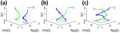
The experimentally measured eigenvalues of different phases for various are plotted in Fig. 3. The braiding behavior is characterized by the following definition of the winding number Nature_Fan :
| (3) |
This number reflects how many times the energy bands are braided. The term here can eliminate the dependence on the choice of reference energy Nature_Fan . So, the winding number defined in Eq. (3) only captures the mutual braiding of the eigenvalues under investigation. Every element of can be expressed as , where is an integer and is the generator. The one-to-one correspondence of exactly describes the behavior. When and , the system is in the unlink phase (Fig. 3(a)). The eigenvalues form two separated curves and in this phase. The two circles can be separated by a line, for example. This is just like a normal insulator in the Hermitian case. If we set the parameters as and , the system will be in the unknot phase, as shown by Fig. 3(b). The two bands interchange as goes from to and in this phase . Note that and are equivalent points and in this phase . Thus two energy bands form a whole circle instead of two circles. For , and and , the eigenvalues form a non-trivial braiding pattern (Fig. 3(c)) and in this phase . The two bands encircle each other and form a structure called the Hopf link. Although in this phase each band forms a circle, they cannot be separated by any line in the complex energy plane as done in the unlink phase.
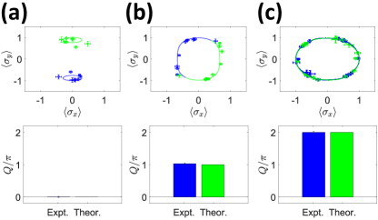
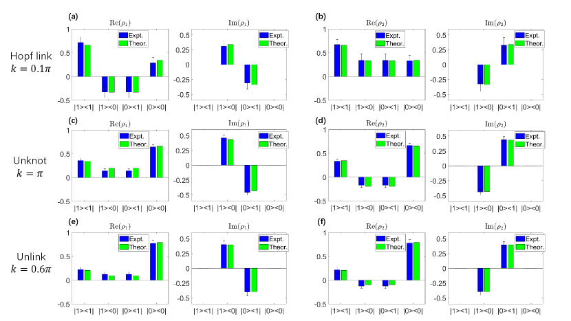
Apart from the non-trivial topology of the energy bands, the global Berry phase determined by the eigenstates was also observed. The global Berry phase is Tr, where the non-abelian Berry connection is defined as Q_Liang . Here () are right (left) eigenstates of an NH Hamiltonian and satisfy the biorthogonal relation . The global Berry phase can identify topological invariance in our model Q_Liang . For the unlink, unknot and Hopf link phases, and , respectively. Figure 4 shows the measured eigenstates projected on the XY plane and they show the same behavior as the eigenvalues. In the unlink phase, form two separated circles on the Bloch sphere, and so are the projections on the XY plane. In the unknot phase, the eigenstates form an end-to-end circle instead, just as the energy bands exchange each other. While in the Hopf link phase, each eigenstates form a closed loop, and the two loops intersect each other. After obtaining from MLE, can be solved from the biorthogonal relation. The experimental value of can be obtained with the method in Ref. ComputeQ via , where and and is the band index. The experimental results of for the unlink, unknot and Hopf link phases are 0.00(2), 1.03(2) and 2.00(3), respectively, which agree well with theoretical predictions. Generally speaking, for bands models with eigenvalues and starting at , the ordered set goes to as varies to . Then we have , where is the parity of the permutation. For our case, both the unlink phase and the Hopf link phase have even parity since each band returns to itself as goes from to . Thus in these two phases mod . Since the energy bands of the unknot phase exchange each other, the parity is odd with mod .
In conclusion, we have experimentally investigated the knot topology in an 1D NH model based on both eigenvalues and eigenstates. The knot structures of eigenvalues, including the unlink, unknot and Hopf link phases, were successfully observed, which manifest the B(2) braid group behavior. The global Berry phase was measured via high fidelity eigenstates, which serves as the knot invariant to identify the parity of band braiding. Our work makes NV center a desirable platform for investigating important non-Hermitian topology. The universality of our dilation method for arbitrary dimensional cases and the ground-state three-level structure of the NV center make it possible to explore the knot topology of three-band models. For 1D models with three bands, the knotted topological phases are described by the conjugate classes of PRL_Haiping ; NatPhys_Bouhon , which host richer topological behaviors since is not commutative when . By introducing more momentum space parameters such as , our platform can be utilized to investigate the knot topology of higher dimensional NH models PRB_Fan ; PRB_ZhiLi .
This work was supported by the National Key R&D Program of China (Grant Nos. 2018YFA0306600 and 2016YFB0501603), the National Natural Science Foundation of China (Grant No. 12174373), the Chinese Academy of Sciences (Grant Nos. XDC07000000 and GJJSTD20200001), Innovation Program for Quantum Science and Technology (Grant No. 2021ZD0302200), Anhui Initiative in Quantum Information Technologies (Grant No. AHY050000) and Hefei Comprehensive National Science Center. X. R. thanks the Youth Innovation Promotion Association of Chinese Academy of Sciences for their support. Ya Wang and Yang Wu thanks the Fundamental Research Funds for the Central Universities for their support.
Yang Wu, Yunhan Wang and Xiangyu Ye contributed equally to this work.
I Appendix A: Experimental Setup
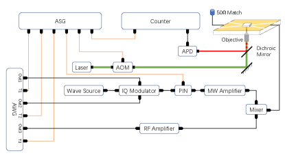
The experimental setup is shown in Fig.5. The diamond was mounted on a confocal setup, and the static magnetic field of 506 G was provided by a permanent magnet along the NV symmetry axis. The initialization and the readout of the NV center spin were realized with a 532 nm green laser controlled by an acousto-optic modulator (AOM) (ISOMET, AOMO 3200-121). The laser beam traveled twice through the acousto-optic modulator before going through an oil objective (Olympus, PLAPON 60*O, NA 1.42) and then focusing on the NV center. The phonon sideband fluorescence (wavelength, 650-800nm) went through the same oil objective and was collected by an avalanche photodiode (Perkin Elmer, SPCM-AQRH-14) with a counter card (NI, PCIe-6612).
The radio-frequency (RF) pulses were generated by an arbitrary waveform generator (AWG) (CIQTEK AWG4100) and were amplified by a power amplifier (Mini-Circuits, LZY-22+). The microwave (MW) pulses were generated by the same arbitrary waveform generator. The bandwidth of the arbitrary waveform generator is 0-330 MHz, which is far from the resonant frequency (about 1.47 GHz). Thus, the pulses were mixed with continuous 1.6-GHz output from a wave source (RIGOL, DSG3065B) using an IQ modulator (Marki, IQ1545LMP). Then the pulses passed a PIN (Mini-Circuits, ZASWA-2-50DRA+) and an amplifier (Mini-Circuits, ZHL-15W-422-S+). Finally both the MW and RF pulses were fed by the same coplanar waveguide after passing the diplexer (Marki, DPX-0R5). The waveforms of MW and RF pulses were prepared in advance and were downloaded to the AWG. An arbitrary sequence generator (CIQTEK ASG8100) was utilized to control the timing in experiment by the trigger signals designed in advance.
II Appendix B: Universal Dilation Method
We use the universal dilation method to construct the NH Hamiltonian Science_YW . Intuitively, by introducing an ancilla system and tuning their interaction in a time-dependent way, the target system obeys the evolution governed by the NH Hamiltonian . The detail can be found in Ref. Science_YW . For an NH Hamiltonian , the dilated Hamiltonian takes the form:
| (4) |
where is the identity matrix and is the Pauli operator on the ancilla. and are operators on the system written as: and . Here and satisfies the following equation:
| (5) |
Now we focus on the realization of in the NV center. The ground state of the NV center can be described by the Hamiltonian
| (6) |
where is the spin-1 operator of the electron (nuclear) spin, GHz is the zero field splitting for the electron, is the electron (nuclear) Zeeman term induced by the magnetic field applied along the NV symmetry axis, MHz is the nuclear quadrupolar interaction, and MHz is the hyperfine interaction. We construct the dilated Hamiltonian in the subspace spanned by the states , and . The Hamiltonian in this subspace can be simplified to
| (7) |
To facilitate the construction of , we further decompose as:
| (8) |
where and are time-dependent coefficients. We apply selective MW pulses to cast the control Hamiltonian:
| (9) |
In order to realize , we choose the rotating frame with the following form:
| (10) |
Thus the Hamiltonian in the rotating frame can be written as
| (11) |
We have omitted the dependence and the integral variable for simplicity, and is the transition frequency of between and ( and ). In order to reduce to under the rotating-wave approximation, the amplitudes, frequencies and phases should satisfy and
| (12) |
The solution reads
| (13) |
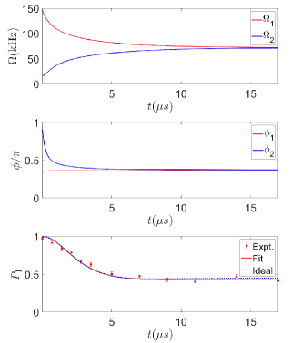
As an example, the result for the Hopf link phase with is shown in Fig. 6. The target NH Hamiltonian is
| (14) | ||||
where , , , and Since the eigenvalues of the Hamiltonian are complex, the state evolution shows a damping behavior and finally reaches one of the eigenstate of the NH Hamiltonian . The dilation procedure gives and to realize the dilated Hamiltonian , as shown in Fig. 6. For an intuitive interpretation, both and first show a decay behavior and then almost remain unchanged. When and are almost equal to their steady value, they effectively act as a rotation along a specific axis determined by the eigenstate of the NH Hamiltonian in the target subspace. The beginning decay part of the control Hamiltonian exactly drives the initial state to be parallel with this rotation axis. The final state thus remains unchanged (in the target subspace) though is not zero. The measured population evolution agrees well with this picture and the theoretical predictions.
III Appendix C: Effects of Dephasing and Crosstalk
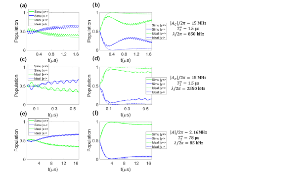
The evolution under the NH Hamiltonian is mainly affected by the dephasing and the crosstalk. Equation 11 shows the ideal case when the two MW pulses are selective. However, in practice the operators in the control Hamiltonian have the form instead of , and the decoherence inevitably undermines the evolution. As mentioned in the main text, one way is to use a strongly coupled 13C nuclear spin. For a natural abundance diamond, the dephasing time ranges from s to s. We take s as a typical value. The coupling strength between the 13C nuclear spin and the electron spin is on the order of 10 MHz generally and we take MHz. The simulation results of the evolution under the basis for the Hopf link phase with and different ’s are shown in Fig. 7. If one uses weak driving to suppress the crosstalk, the evolution time is s, which is comparable to the coherence time. The decoherence drastically destroys the coherent evolution. The population evolution under bases is shown in Figs. 7(a) and 7 (b), which greatly deviates from the ideal case. We use to characterize the coherence. In this parameter configuration, for the final state we have and for the ideal case we have . Only about 67% coherence is left. One may try to set a large value of under which the time needed to reach the steady state is within the coherence time. When varies from kHz to kHz, increases from 0.057 to 0.17 and the evolution time needed decreases from s to s. The pulses are no longer selective and the evolution is significantly affected by the crosstalk. As can be seen from Fig. 7(c) and 7(d), the system can barely reach a steady state.
Another way is to use samples in which the NV center has a long coherence time. For our sample, fitting of the luminescence in the Ramsey experiment shows that s (see main text). Fig. 7(e) and 7(f) show the simulation results for our parameters where we take s. Here MHz is a typical value for the coupling strength between the 14N nuclear spin and the electron spin. For this parameter configuration, . The deviation caused by decoherence and crosstalk is about 0.03 and these effects on the fidelity between the final states in experiments and the ideal eigenstates can be ignored.
IV Appendix D: Experimental Acquisition of the Eigenstates
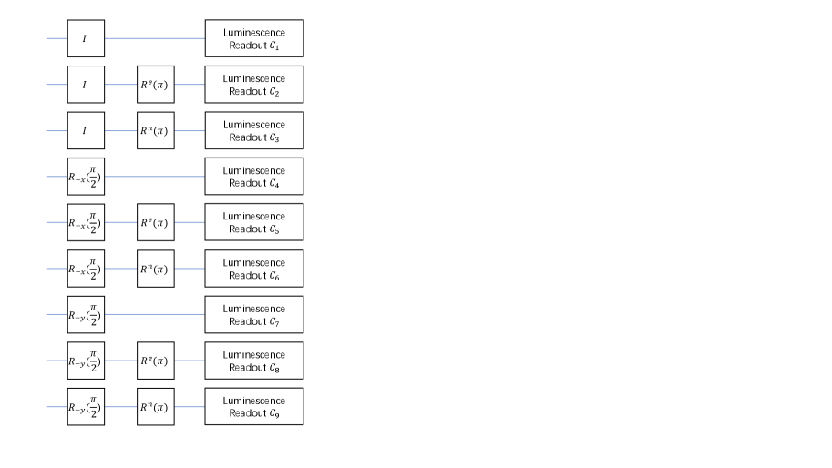
For the final state of the evolution, nine different measurement sequences are applied to reconstruct the state (Fig. 8). Here is the pulse on the electron spin in the subspace and is the pulse on the nuclear spin in the subspace. and correspond to the transition MW1 and RF2, respectively, in Fig.2(d) of the main text. The pulses rotate the electron spin in both spaces. We use normalization sequences to obtain the PL rate for each of the four levels PRL_Wenquan . The contribution for the counts of each level is the PL rate multiplied by the corresponding population. The count of each measurement sequence equals the summation of the contribution over each level. By solving the equations that relate the populations of each level under different bases and counts for each measurement sequence, we can obtain the expectation values of the final state.
From of the final state, we can directly reconstruct by , but the direct result may give a mixed state or even an unphysical state. Thus the maximum likelihood estimation has been utilized to obtain the pure states from the experimental results. We parameterize the pure state as , where all parameters are real and satisfy the normalization condition. Note that the measurement result of each sequence is determined by the population on each level. Since and reverse the population of the corresponding levels, the phase difference between the two subspace does not manifest in the measurement result. Here we fix the coefficients of to be real to eliminate the irrelevant phase freedom, since we only need the results in the subspace. Then the expectation values for the nine counts can be obtained from the PL rates and the parameters of the pure state, where we label the levels , and as and for simplicity. For example, the expectation values for the counts of the first and second sequences read and . Then the loss function is chosen to be
| (15) |
where are the measured counts for each sequence. Optimize these parameters to minimize and we obtain the pure state up to a normalization factor. Here the subscript means the parameters that minimize . The experimentally obtained fidelities of all the eigenstates exceed 0.97. Based on the model parameters given in the main text, we show the results of some eigenstates as examples in Fig.r̃efSFig3. The corresponding fidelities are as follows: Hopf link, 1.00(7) and 1.00(6) for and (same below) at ; unknot, 1.00(2) and 1.00(3) at and unlink, 1.00(3) and 1.00(3) at .
References
- (1) E. J. Bergholtz, J. C. Budich, and F. K. Kunst, Exceptional topology of non-Hermitian systems, Rev. Mod. Phys. 93, 015005 (2021).
- (2) S. Yao, and Z. Wang, Edge states and topological invariants of non-Hermitian systems, Phys. Rev. Lett. 121, 086803 (2018).
- (3) K. Kawabata, K. Shiozaki, M. Ueda, and M. Sato, Symmetry and topology in non-Hermitian physics, Phys. Rev. X 9, 041015 (2019).
- (4) Z. Gong, Y. Ashida, K. Kawabata, K. Takasan, S. Higashikawa, and M. Ueda, Topological phases of non-Hermitian systems, Phys. Rev. X 8, 031079 (2018).
- (5) T. E. Lee, Anomalous edge state in a non-Hermitian lattice, Phys. Rev. Lett. 116, 133903 (2016).
- (6) H. Zhou, C. Peng, Y. Yoon, C. W. Hsu, K. A. Nelson, L. Fu, J. D. Joannopoulos, M. Soljai, and B. Zhen, Observation of bulk Fermi arc and polarization half charge from paired exceptional points, Science 359, 1009-1012 (2018).
- (7) J. Carlstrm, and E. J. Bergholtz, Exceptional links and twisted Fermi ribbons in non-Hermitian systems, Phys. Rev. A 98, 042114 (2018).
- (8) B. Peng, Ş. K. zdemir, F. Lei, F. Monifi, M. Gianfreda, G. L. Long, S. Fan, F. Nori, C. M. Bender, and L. Yang, Parity-time-symmetric whispering-gallery microcavities, Nature Physics 10, 394-398 (2014).
- (9) L. Feng, M. Ayache, J. Huang, Y.-L. Xu, M.-H. Lu, Y.-F. Chen, Y. Fainman, and A. Scherer, Nonreciprocal light propagation in a silicon photonic circuit, Science 333, 729-733 (2011).
- (10) L. Feng, Z. J. Wong, R.-M. Ma, Y. Wang, and X. Zhang, Single-mode laser by parity-time symmetry breaking, Science 346, 972-975 (2014).
- (11) H. Hodaei, M.-A. Miri, M. Heinrich, D. N. Christodoulides, and M. Khajavikhan, Parity-time-symmetric microring lasers, Science 346, 975-978 (2014).
- (12) R. El-Ganainy, K. G. Makris, M. Khajavikhan, Z. H. Musslimani, S. Rotter, and D. N. Christodoulides, Non-Hermitian physics and PT symmetry, Nature Physics 14, 11-19 (2018).
- (13) K. G. Makris, R. El-Ganainy, D. N. Christodoulides, and Z. H. Musslimani, Beam Dynamics in PT Symmetric Optical Lattices, Phys. Rev. Lett. 100, 103904 (2008).
- (14) H. Jing, S. K. zdemir, X.-Y. L, J. Zheng, L. Yang, and F. Nori, PT-Symmetric Phonon Laser, Phys. Rev. Lett. 113, 053604 (2014).
- (15) J. M. Zeuner, M. C. Rechtsman, Y. Plotnik, Y. Lumer, S. Nolte, M. S. Rudner, M. Segev, and A. Szameit, Observation of a topological transition in the bulk of a non-Hermitian system, Phys. Rev. Lett. 115, 040402 (2015).
- (16) L. Feng, R. El-Ganainy, and L. Ge, Non-Hermitian photonics based on parity-time symmetry, Nature Photonics 11, 752-762 (2017).
- (17) A. Regensburger, C. Bersch, M.-A. Miri, G. Onishchukov, D. N. Christodoulides, and U. Peschel, Parity-time synthetic photonic lattices, Nature 488, 167-171 (2012).
- (18) B. Peng, Ş. K. zdemir, S. Rotter, H. Yilmaz, M. Liertzer, F. Monifi, C. M. Bender, F. Nori, and L. Yang, Loss-induced suppression and revival of lasing, Science 346, 328-332 (2014).
- (19) R. Fleury, D. Sounas, and A. Al, An invisible acoustic sensor based on parity-time symmetry, Nature Commun. 6, 5905 (2015).
- (20) T. Liu, X. Zhu, F. Chen, S. Liang, and J. Zhu, Unidirectional Wave Vector Manipulation in Two-Dimensional Space with an All Passive Acoustic Parity-Time-Symmetric Metamaterials Crystal, Phys. Rev. Lett. 120, 124502 (2018).
- (21) Z. Zhang, M. R. Lpez, Y. Cheng, X. Liu, and J. Christensen, Non-Hermitian Sonic Second-Order Topological Insulator, Phys. Rev. Lett. 122, 195501 (2019).
- (22) I. Rotter, A non-Hermitian Hamilton operator and the physics of open quantum systems, J. Phys. A 42, 153001 (2009).
- (23) B. Zhen, C. W. Hsu, Y. Igarashi, L. Lu, I. Kaminer, A. Pick, S.-L. Chua, J. D. Joannapoulos, and M. Soljai, Spawning rings of exceptional points out of Dirac cones, Nature 525, 354-358 (2015).
- (24) H. J. Carmichael, Quantum trajectory theory for cascaded open systems, Phys. Rev. Lett. 70, 2273 (1993).
- (25) S. Diehl, E. Rico, M. A. Baranov, and P. Zoller, Topology by dissipation in atomic quantum wires, Nature Physics 7, 971-977 (2011).
- (26) V. Kozii, and L. Fu, Non-hermitian topological theory of finite-lifetime quasiparticles: Prediction of bulk Fermi arc due to exceptional point, arXiv:1708.05841.
- (27) T. Yoshida, R. Peters, and N. Kawakami, Non-Hermitian perspective of the band structure in heavy-fermion systems, Phys. Rev. B 98, 035141 (2018).
- (28) H. Shen, and L. Fu, Quantum oscillation from in-gap states and a non-Hermitian Landau level problem, Phys. Rev. Lett. 121, 026403 (2018).
- (29) M. Papaj, H. Isobe, and L. Fu, Nodal arc of disordered Dirac fermions and non-Hermitian band theory, Phys. Rev. B 99, 201107(R) (2019).
- (30) K. Zhang, Z. Yang, and C. Fang, Correspondence between winding numbers and skin modes in non-Hermitian systems, Phys. Rev. Lett. 125, 126402 (2020).
- (31) D. S. Borgnia, A. J. Kruchkov, and R.-J. Slager Non-Hermitian boundary modes and topology, Phys. Rev. Lett. 124, 056802 (2020).
- (32) N. Okuma, K. Kawabata, K. Shiozaki, and M. Sato, Topological origin of non-Hermitian skin effects, Phys. Rev. Lett. 124, 086801 (2020).
- (33) C. C. Wojcik, X.-Q. Sun, T. Bzduek, and S. Fan, Homotopy characterization of non-Hermitian Hamiltonians, Phys. Rev. B 101, 205417 (2020).
- (34) H. Hu, and E. Zhao, Knots and non-Hermitian Bloch bands, Phys. Rev. Lett. 126, 010401 (2021).
- (35) Z. Li, and R. S. K. Mong, Homotopical characterization of non-Hermitian band structures, Phys. Rev. B 103, 155129 (2021).
- (36) K. Wang, A. Dutt, C. C. Wojcik, and S. Fan, Topological complex-energy braiding of non-Hermitian bands, Nature 598, 59-64 (2021).
- (37) Y. S. S. Patil, J. Hller, P. A. Henry, C. Guria, Y. Zhang, L. Jiang, N. Kralj, N. Read, and J. G. E. Harris, Measuring the knot of non-Hermitian degeneracies and non-commuting braids, Nature 607, 271-275 (2022).
- (38) M.-M. Cao, K. Li, W.-D. Zhao, W.-X. Guo, B.-X. Qi, X.-Y. Chang, Z.-C. Zhou, Y. Xu, and L.-M. Duan, Probing complex-energy topology via non-Hermitian absorption spectroscopy in a trapped ion simulator, Phys. Rev. Lett. 130, 163001 (2023).
- (39) Y. Wu, W. Liu, J. Geng, X. Song, X. Ye, C. Duan, X. Rong, and J. Du, Observation of parity-time symmetry breaking in a single-spin system, Science 364, 878-880 (2019).
- (40) W. Zhang, X. Ouyang, X. Huang, X. Wang, H. Zhang, Y. Yu, X. Chang, Y. Liu, D.-L. Deng, and L.-M. Duan, Observation of non-Hermitian topology with non-unitary dynamics of solid-state spins, Phys. Rev. Lett. 127, 090501 (2021).
- (41) U. Gnther, and B. F. Samsonov, Naimark-dilated PT-symmetric brachistochrone, Phys. Rev. Lett. 101, 230404 (2008).
- (42) K. Kawabata, Y. Ashida, and M. Ueda, Information retrieval and criticality in parity-time-symmetric systems, Phys. Rev. Lett. 119, 190401 (2017).
- (43) V. Jacques, P. Neumann, J. Beck, M. Markham, D. Twitchen, J. Meijer, F. Kaiser, G. Balasubramanian, F. Jelezko, and J. Wrachtrup, Dynamic polarization of single nuclear spins by optical pumping of nitrogen-vacancy color centers in diamond at room temperature, Phys. Rev. Lett. 102, 057403 (2009).
- (44) S.-D. Liang, and G.-Y. Huang, Topological invariance and global Berry phase in non-Hermitian systems, Phys. Rev. A 87, 012118 (2013).
- (45) T. Fukui, Y. Hatsugai, and H. Suzuki, Chern numbers in discretized brillouin zone: Efficient method of computing (spin) hall conductances, J. Phys. Soc. Jpn. 74, 1674-1677 (2005).
- (46) A. Bouhon, Q. Wu, R.-J. Slager, H. Weng, O. V. Yazyev, and T. Bzdusek, Non-Abelian reciprocal braiding of Weyl points and its manifestation in ZrTe, Nature Physics 16, 1137–1143 (2020)
- (47) W. Liu, Y. Wu, C. Duan, X. Rong, and J. Du, Dynamically encircling an exceptional point in a real quantum system. Phys. Rev. Lett. 126, 170506 (2021).