Observation of spin-space quantum transport
induced by an atomic quantum point contact

Figure 2a shows the time evolution of the spin precession in the absence of the $\ket{e}$ atom, exhibiting the coherent oscillation of Ramsey signals with the frequency corresponding to the differential Raman light shift between $\ket{\uparrow}$ and $\ket{\downarrow}$ states (see Methods). As shown in Fig. 2b, on the other hand, the damping of the oscillation is observed in the presence of the $\ket{e}$ atom, indicating that the impurity-induced quantum transport is successfully demonstrated. Figure 2c represents the observed oscillation amplitude $A(t)$ as functions of the hold time. The oscillation amplitude is associated with the spin polarization, defined as $\Delta N/N$, where $\Delta N=N_{+}-N_{-}$ and $N=N_{+}+N_{-}$, with $N_{\sigma}$ being the number of atoms in the $\ket{\sigma}$ state. After the second Raman pulse of $R_{\pi-\theta}$, $N_{+}$ and $N_{-}$ correspond to $N_{\uparrow}$ and $N_{\downarrow}$, respectively. Thus, using the measured quantities of $N_{\uparrow}$ and $N_{\downarrow}$, $N_{\uparrow}/N=N_{\uparrow}/(N_{\uparrow}+N_{\downarrow})$ and $\Delta N/N=(N_{\uparrow}-N_{\downarrow})/(N_{\uparrow}+N_{\downarrow})$ can be extracted. See Methods for the detail of the procedure of extracting $N_{\uparrow}/N$ and $\Delta N/N$ from the measurements. We focus on the transport dynamics after 10 ms, where $N_{-}$, being the number of atoms in the drain, becomes of the order of ten and enough to justify thermodynamic treatments [25]. The transient regime is also determined by the thermalization rate, which depends on the atom density, the scattering cross section and the atom velocity. The thermalization rate is estimated as 100 Hz, corresponding to the transition regime of $t<$10 ms. We confirm the ohmic conduction, which manifests itself as the exponential decay of the oscillation amplitude with the finite lifetime of the $\ket{e}$ state taken into consideration (see Methods), and the decoherence rate is obtained as $\gamma=47(4)$ Hz from the data fits. We note that the 25 % reduction of $N$ was observed during the hold time of 40 ms, which is comparable with the $\ket{e}$-atom number loss, suggesting that the loss is caused by the inelastic collision between the $\ket{e}$ and $\ket{g}$ atoms. After 10 ms hold time, which is the temporal region of our interest, however, the reduction of $N$ is only about 8 %, comparable to the uncertainty of the measurements, and thus is not taken into consideration in the analysis. The measured decoherence rate is larger than the decay rate of the $\ket{e}$ atom and smaller compared to the thermalization rate, suggesting that a quasi-steady approximation is applicable, where $N_{\mathrm{imp}}$ and $\mu_{\pm}$ in Equation (3) are replaced with those at the instantaneous time $t$. In contrast, the data at early time deviates from the data fits after 10 ms, implying the nonlinear nature of the transport dynamics. The quantitative explanation including these data is an interesting future theory work.

More directly, we can confirm the ohmic conduction from the linearity between the current and chemical potential bias. The current $I_{+\to-}$ which flows from $\ket{+}$ to $\ket{-}$ is defined as

and thus can be extracted from the slope for $\Delta N$ in Fig. 2c. It is noted that the factor 1/2 in Equation (5) accounts for the double counting of the decreased atom number in the $\ket{+}$ state and the increased atom number in the $\ket{-}$ state. Here $N_{+}$ and $N_{-}$ can be rewritten as functions of $\mu_{+}$ and $\mu_{-}$ based on the thermodynamics in 1D trapped fermions (see Methods). Circles in Fig. 2d show thus obtained chemical-potential-bias dependence of the current. Because of the finite lifetime of the $\ket{e}$ atom, the finite chemical potential bias $\Delta\mu$ is present even when the current asymptotically approaches to zero. In order to compensate for this finite lifetime effect, we multiply the observed current by the factor $e^{+t/\tau}$, which leads to $I_{+\to-}=\gamma\Delta N$ shown as squares in Fig. 2d. As a result, we obtain the linear dependence between the current and chemical potential bias, indicating the ohmic conduction. The conductance, defined as $I_{+\to-}=G\Delta\mu$, is obtained as $G=0.45/h$.

We theoretically estimate the conductance from the numerical calculation of the transport dynamics, shown as a dashed line in Fig. 2c. In the calculation, we take into account the spatial inhomogeneity of the atom numbers among many tubes, and the total atom-number difference $\Delta N_{\mathrm{tot}}$ is expressed as

where $i$ means the index of the tube, and $\Delta N_{i}$ and $\mu_{i\pm}$ correspond to the atom-number difference and the chemical potentials for the $\ket{\pm}$ states in the $i$-th tube, respectively. As a result, we obtain $G=0.41/h$, which is consistent with the measured value (see Supplementary Fig. 3).

Figure 2e shows the impurity-fraction dependence of the spin-flip rate, revealing that the spin-flip rate is proportional to $\rho_{\mathrm{imp}}=N_{\mathrm{imp}}(t=0)/N$. This is consistent with our expectation that each impurity atom serves as a single-mode QPC and the overall transport current should be proportional to the number of impurity atoms. Based on this linear dependence, the single-impurity conductance is estimated as $G_{0}=4.1\times 10^{-2}/h$. By increasing the sensitivity of our experiment, the low impurity-fraction limit of this measurement will reveal the conductance discretized in units of $G_{0}$, namely in the form of $N_{\mathrm{imp}}G_{0}$, expected from the Landauer-Büttiker formula.

We investigate how the quantum transport dynamics depends on the choice of the basis sets of the spin states. In Fig. 2, we consider the basis set of $\ket{+}$ and $\ket{-}$ created by rotation $R_{\theta=\pi/2}$, but in general we can consider basis sets created by $R_{\theta}$ with any value of $\theta$. The generalization of the Equation (4) for arbitrary $\theta$ is straightforward, and is given as [14]:

indicating that the $\theta$ dependence of the transport current is expected to be proportional to $\sin^{2}\theta$. Figure 3a shows the transport dynamics with different rotation angles in a magnetic field of 45 Gauss, exhibiting the clear $\theta$ dependence. Quantitatively, the spin-flip rate is obtained as the slope of the fitting curve at the initial time $t=0$. Figure 3b shows the obtained spin-flip rate as a function of the rotation angle, which is in agreement with the expected $\sin^{2}\theta$ dependence.

Since the QPC in this scheme is provided by individual atoms in the $\ket{e}$ state, rather than the channel structure, the quantum transport can be controlled by the excitation and de-excitation for the $\ket{e}$ atom. Figure 4a summarizes the time-resolved control of transport dynamics observed with the pulse sequences depicted in Figs. 4b-d. The experiment is performed in a magnetic field of 45 Gauss. The pulse sequence (b) illustrates the typical transport experiment similar to Fig. 2b. In the pulse sequence (c), after the transport time of 5 ms, we return the $\ket{e}$ atoms back to the $\ket{g}$ state by shining the repumping light which is resonant with the ${}^{3}\mathrm{P}_{0}$–${}^{3}\mathrm{D}_{1}$ transition. This can be regarded as an operation of $\pi$ pulse in the control qubit in the quantum circuit model of Fig. 1b. The result clearly shows the suppression of the transport. Note that the atoms should return to the ground state via several spontaneous emissions with no preferential spin components, and thus they neither contribute to the creation of spin coherence nor the decoherence. In the pulse sequence (d), after shining the repumping light we wait for 35 ms, and then apply the clock excitation pulse again to transfer the atoms in the $\ket{-5/2}$ state to the $\ket{e}$ state. As shown in Fig. 4a, the revival of the transport dynamics is observed, demonstrating the dynamical switching of the quantum transport almost at will with the excitation and de-excitation pulses.

Furthermore, we investigate the possibility of controlling the spin-dependent interaction responsible for the quantum transport. Owing to the existence of the orbital Feshbach resonance between the $\ket{g}$ and $\ket{e}$ atoms of ${}^{173}\mathrm{Yb}$, the scattering phase shift depends on a magnetic field, suggesting the tunability of the transport current with a magnetic field. Figures 5a-b show the transport dynamics in a magnetic field of (a) 45 Gauss and (b) 135 Gauss for various impurity fractions $\rho_{\mathrm{imp}}$, showing that the transport current depends on the magnetic field. The result of the numerical calculation of the phase shift difference, associated with the transmittance, is consistent with the faster transport dynamics observed in a magnetic field of 135 Gauss than in 45 Gauss (see Supplementary Fig. 2). We repeat a similar transport measurement using ${}^{171}\mathrm{Yb}$ which does not show an orbital Feshbach resonance in the magnetic field range of the present experiment [31]. The result shows much slow decoherence consistent with the expectation.

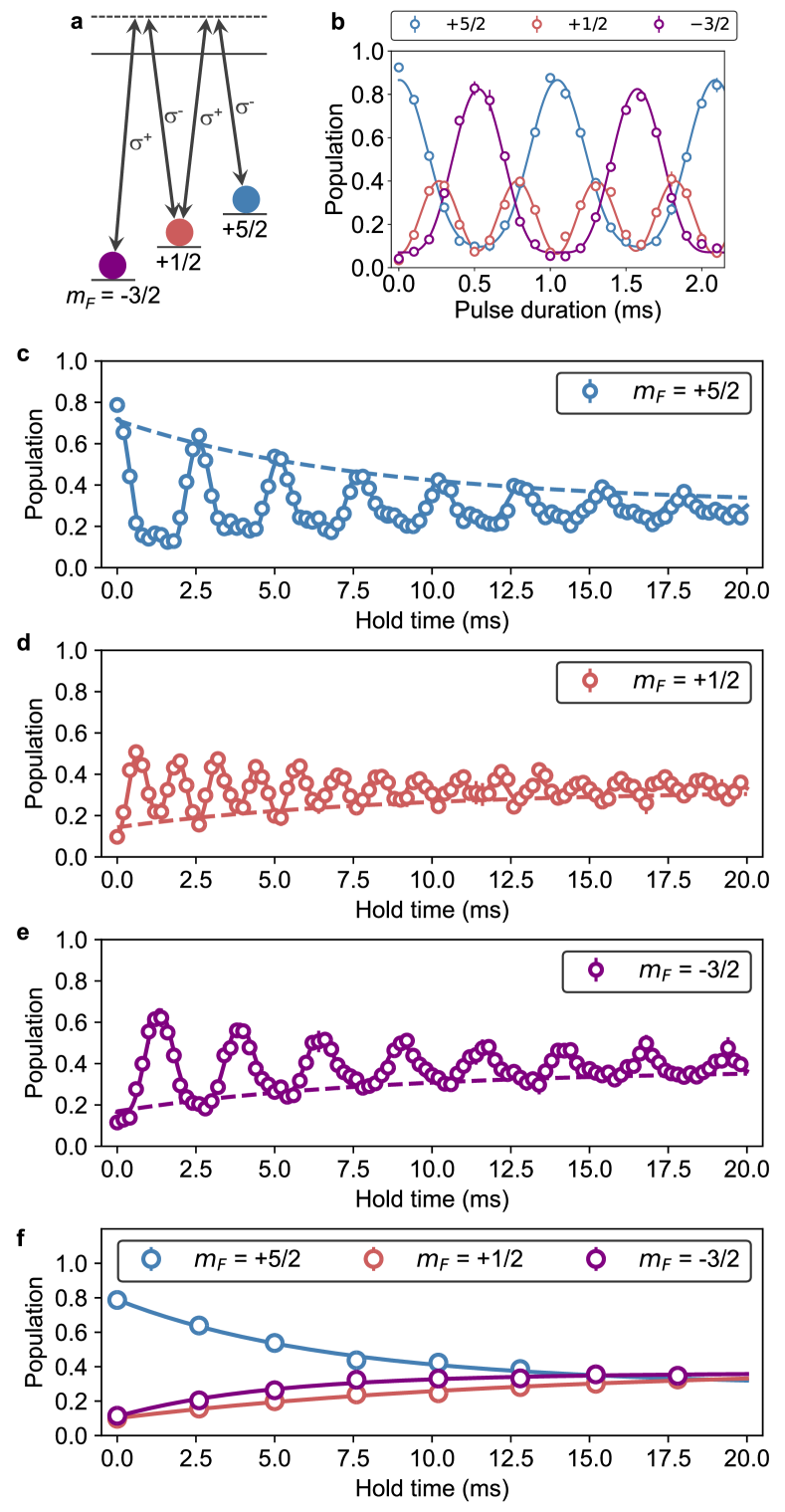
The high spin degrees of freedom of ${}^{173}\mathrm{Yb}$ with SU($\mathcal{N}\leq 6$) symmetry allow one to study the multi-terminal quantum transport system up to 6. Here the SU($\mathcal{N}$) symmetry is crucial, because otherwise the spin-changing collisions take place and the system shows spin dynamics even without the localized impurities [26]. We realize the three-terminal quantum transport system by coherently connecting the $\ket{+5/2}$, $\ket{+1/2}$, and $\ket{-3/2}$ states as shown in Fig. 6a. This corresponds to the Y-junction, which has been studied theoretically [27, 28] and experimentally [29, 30]. We prepare the superposition with almost equal weights of the three $m_{F}$ states with the Raman pulse with the duration of $t_{0}=0.31$ ms (see Fig. 6b for the Raman Rabi oscillation). After the transport time, the second Raman pulse is applied with the pulse duration of $T-t_{0}$, and the spin population is detected in the original basis. Here $T=1.06$ ms denotes the period of the Raman Rabi oscillation. It is noted that the remaining $\ket{g}$ atoms in the $\ket{-5/2}$ state are removed using the light resonant with the ${}^{1}\mathrm{S}_{0}$–${}^{3}\mathrm{P}_{1}$($F^{\prime}=7/2$) transition since the remaining atom is undesirably coupled with the $\ket{-1/2}$ state via the Raman transition.

Figures 6c-e show the time evolution of the spin population in the presence of the $\ket{e}$ atom in a magnetic field of 119 Gauss, which clearly exhibit the decoherence of the spin precession. In the absence of the $\ket{e}$ atom, the coherent oscillation is observed with no discernible decoherence up to at least 40 ms. In Fig. 6f, the spin populations at several transport times are plotted. The number of the terminals can be increased up to 6 by fully utilizing the spin degrees of freedom of ${}^{173}\mathrm{Yb}$.

A 2D array of the 1D tubes is produced using the 2D state-independent optical lattice with the wavelength of 759.4 nm. The 1D near-resonant optical lattice is superimposed along the axis of the tubes. The wavelength of the near-resonant optical lattice is chosen to be 650.7 nm, close to the ${}^{3}\mathrm{P}_{0}$–${}^{3}\mathrm{S}_{1}$ transition wavelength of 649.1 nm, giving the strong confinement to the $\ket{e}$ atom alone and no net effect to the $\ket{g}$ atom [19].

After the preparation of the two-component Fermi gas ($\ket{\pm 5/2}$) with the typical atom number $4\times 10^{4}$ and the temperature $0.2T_{\mathrm{F}}$, where $T_{\mathrm{F}}$ is the Fermi temperature, the atoms are adiabatically loaded into the optical lattices, resulting in the 2D array of about $1\times 10^{3}$ 1D tubes with a typical atom number of 30 per tube. The initial lattice depths of the 2D-magic-wavelength optical lattice and the 1D near-resonant optical lattice are set to 30$E_{\mathrm{R}}$ and $6.8E_{\mathrm{R}}$ for the $\ket{e}$ atom, respectively, where $E_{\mathrm{R}}=h\times 2.0$ kHz represents the recoil energy for the magic wavelength. After the coherent transfer to the $\ket{e}$ state, the near resonant optical lattice is ramped up to $27E_{\mathrm{R}}$ to localize the $\ket{e}$ atoms. The axial and radial trap frequencies for the ground state are 76 Hz and 22 kHz, respectively, and those for the excited state 24 kHz and 22 kHz, respectively. In this system, the $\ket{g}$ atom can be regarded as a 1D fermion since the radial vibrational energy is much larger than the Fermi energy in the central tube, which is estimated as $h\times 2$ kHz.

The atom in the $\ket{g}\ket{-5/2}$ state is coherently excited to the $\ket{e}\ket{-5/2}$ state with $\pi$-polarized light in a magnetic field, which is kept constant during the transport dynamics. The Rabi frequency of the clock excitation is $2\pi\times 2.5$ kHz, and the impurity fraction $\rho_{\mathrm{imp}}$ is tuned by choosing the pulse duration from 70 to 200 $\mu$s. The excitation laser is stabilized using an ultra-low-expansion glass cavity [35], and the typical linewidth is a few Hz.

In the two-terminal experiment, the Raman light is blue-detuned by 1.00 GHz from the ${}^{3}\mathrm{P}_{1}$ ($F’=7/2$) state, and the polarization is perpendicular to the quantization axis defined by the magnetic field, and this results in an equal mixture of $\sigma^{+}$ and $\sigma^{-}$ polarization, realizing the Raman transition between the $\ket{+5/2}$ and $\ket{+1/2}$ states. Note that the spin-dependent light shifts induced by the Raman light alter the resonance frequency of the $\ket{+5/2}\leftrightarrow\ket{+1/2}$ Raman transition, resulting in the oscillatory behavior of the Ramsey signal, as shown in Figs. 2a and b. They also make the otherwise resonant transition to the $\ket{-3/2}$ state off-resonant and suppressed.

In the three-terminal experiment, in contrast, the Raman light is blue-detuned by 3.35 GHz from the ${}^{3}\mathrm{P}_{1}$ ($F’=7/2$) state, and the polarization is an equal mixture of $\pi$, $\sigma^{+}$, and $\sigma^{-}$ polarization, resulting in the equal level spacing of the $\ket{g}$ state manifold. The oscillatory behavior of the Ramsey signal shown in Fig. 6 also comes from the spin-dependent light shifts induced by the Raman light.

The spin population is detected with the optical Stern-Gerlach (OSG) method [24], where a spin-dependent optical potential gradient is applied to separately observe the atoms in the different $\ket{m_{F}}$ states. The circularly polarized OSG light propagated along the quantization axis is blue-detuned by 1.13 GHz from the ${}^{3}\mathrm{P}_{1}$ ($F’=7/2$) state. The non-negligible photon scattering associated with the OSG light results in the production of the small number of otherwise non-existing spin components. We include the number of these spin components in the analysis, although it is typically less than 15 percent.

The oscillation amplitude $A(t)$ at the hold time $t$ is obtained from the fit to the data in the time interval $t^{\prime}\in[t,t+1\;\text{ms}]$ with the following function $(N_{\uparrow}/N)_{\text{meas}}=A(t)\cos(\omega(t)t^{\prime}+\varphi(t))+B(t)$, where $\omega(t)$, $\varphi(t)$, and $B(t)\approx 1/2$ correspond to the precession angular frequency, the oscillation phase, and the offset, respectively. In addition, to compensate for the systematic effects associated with the detection process, we introduce the normalization of $2A(t)$ by its maximum value of $2A(t)|_{\text{max}}$. We then obtain $N_{\uparrow}/N=1/2+A(t)/(2A(t)|_{\text{max}})$.

From Equations (3) and (5) for the two-terminal system, the time derivative of $\Delta N$ is found to be proportional to $\Delta N$ when the current is linearized in terms of $\Delta\mu\propto\Delta N$, and the oscillation amplitude of the spin precession corresponds to $\Delta N/N$ as is mentioned in the main text. In order to analyze the transport dynamics quantitatively, the finite lifetime of the $\ket{e}$ atom $\tau$ is taken into consideration by introducing the time-dependent damping factor $e^{-t/\tau}$. Consequently, the oscillation amplitude $A(t)$ satisfies the following differential equation in terms of the transport time $t$:

where $\gamma$ is associated with the decoherence rate. Solving Equation (8) yields

Except for the data fits in Fig. 5b, $\tau$ is fixed to the measured lifetime of the $\ket{e}$ atom during the transport dynamics, which is 60 ms in a magnetic field of 45 Gauss.

The partition function is expressed as

where $\varepsilon_{n}=\hbar\omega_{\mathrm{trap}}n$ $(n=0,1,2,...)$. Here $\omega_{\mathrm{trap}}=2\pi\times 76$ Hz is the axial trap frequency of the tube potential. Thus the grand potential is obtained as

where $\mathrm{Li}_{n}(z)$ is the polylogarithm function. In this calculation, a continuous approximation $\beta\hbar\omega_{\mathrm{trap}}\to 0$ is applied to convert the sum over $n$ in $\log Z$ to an integral. Using Equation (11), the number of the atoms in the $\ket{\sigma}$ state can be given by

References

- [1] Imry, Y. Introduction to mesoscopic physics (Oxford University Press, 2002).
- [2] Ihn, T. Semiconductor Nanostructures: Quantum states and electronic transport (Oxford University Press, 2010).
- [3] Bloch, I., Dalibard, J. & Nascimbène, S. Quantum simulations with ultracold quantum gases. Nature Physics 8, 267–276 (2012).
- [4] Chien, C.-C., Peotta, S. & Di Ventra, M. Quantum transport in ultracold atoms. Nature Physics 11, 998–1004 (2015).
- [5] Krinner, S., Esslinger, T. & Brantut, J.-P. Two-terminal transport measurements with cold atoms. Journal of Physics: Condensed Matter 29, 343003 (2017).
- [6] Amico, L. et al. Roadmap on Atomtronics: State of the art and perspective. Preprint at https://arxiv.org/abs/2008.04439v5 (2021).
- [7] Landauer, R. Spatial variation of currents and fields due to localized scatterers in metallic conduction. IBM Journal of Research and Development 1, 223–231 (1957).
- [8] Büttiker, M., Imry, Y., Landauer, R. & Pinhas, S. Generalized many-channel conductance formula with application to small rings. Phys. Rev. B 31, 6207–6215 (1985).
- [9] Krinner, S., Stadler, D., Husmann, D., Brantut, J.-P. & Esslinger, T. Observation of quantized conductance in neutral matter. Nature 517, 64–67 (2015).
- [10] Husmann, D. et al. Connecting strongly correlated superfluids by a quantum point contact. Science 350, 1498–1501 (2015).
- [11] Knap, M. et al. Time-dependent impurity in ultracold fermions: Orthogonality catastrophe and beyond. Phys. Rev. X 2, 041020 (2012).
- [12] Nishida, Y. Transport measurement of the orbital kondo effect with ultracold atoms. Phys. Rev. A 93, 011606 (2016).
- [13] You, J.-S., Schmidt, R., Ivanov, D. A., Knap, M. & Demler, E. Atomtronics with a spin: Statistics of spin transport and nonequilibrium orthogonality catastrophe in cold quantum gases. Phys. Rev. B 99, 214505 (2019).
- [14] Nakada, S., Uchino, S. & Nishida, Y. Simulating quantum transport with ultracold atoms and interaction effects. Phys. Rev. A 102, 031302 (2020).
- [15] Sommer, A., Ku, M., Roati, G. & Zwierlein, M. W. Universal spin transport in a strongly interacting fermi gas. Nature 472, 201–204 (2011).
- [16] Koschorreck, M., Pertot, D., Vogt, E. & Köhl, M. Universal spin dynamics in two-dimensional fermi gases. Nature Physics 9, 405–409 (2013).
- [17] Krinner, S. et al. Mapping out spin and particle conductances in a quantum point contact. Proceedings of the National Academy of Sciences 113, 8144–8149 (2016).
- [18] Luciuk, C. et al. Observation of quantum-limited spin transport in strongly interacting two-dimensional fermi gases. Phys. Rev. Lett. 118, 130405 (2017).
- [19] Ono, K., Amano, Y., Higomoto, T., Saito, Y. & Takahashi, Y. Observation of spin-exchange dynamics between itinerant and localized atoms. Phys. Rev. A 103, L041303 (2021).
- [20] Mancini, M. et al. Observation of chiral edge states with neutral fermions in synthetic hall ribbons. Science 349, 1510–1513 (2015).
- [21] Zhang, R., Cheng, Y., Zhai, H. & Zhang, P. Orbital feshbach resonance in alkali-earth atoms (2015).
- [22] Pagano, G. et al. Strongly interacting gas of two-electron fermions at an orbital feshbach resonance. Phys. Rev. Lett. 115, 265301 (2015).
- [23] Höfer, M. et al. Observation of an orbital interaction-induced feshbach resonance in . Phys. Rev. Lett. 115, 265302 (2015).
- [24] Taie, S. et al. Realization of a system of fermions in a cold atomic gas. Phys. Rev. Lett. 105, 190401 (2010).
- [25] Pagano, G. et al. A one-dimensional liquid of fermions with tunable spin. Nature Physics 10, 198–201 (2014).
- [26] Krauser, J. S. et al. Coherent multi-flavour spin dynamics in a fermionic quantum gas. Nature Physics 8, 813–818 (2012).
- [27] Nayak, C., Fisher, M. P. A., Ludwig, A. W. W. & Lin, H. H. Resonant multilead point-contact tunneling. Phys. Rev. B 59, 15694–15704 (1999).
- [28] Tokuno, A., Oshikawa, M. & Demler, E. Dynamics of one-dimensional bose liquids: Andreev-like reflection at junctions and the absence of the aharonov-bohm effect. Phys. Rev. Lett. 100, 140402 (2008).
- [29] Li, J., Papadopoulos, C. & Xu, J. Growing y-junction carbon nanotubes. Nature 402, 253–254 (1999).
- [30] Papadopoulos, C., Rakitin, A., Li, J., Vedeneev, A. S. & Xu, J. M. Electronic transport in y-junction carbon nanotubes. Phys. Rev. Lett. 85, 3476–3479 (2000).
- [31] Bettermann, O. et al. Clock-line photoassociation of strongly bound dimers in a magic-wavelength lattice. Preprint at https://arxiv.org/abs/2003.10599 (2020).
- [32] Yamamoto, R., Kobayashi, J., Kuno, T., Kato, K. & Takahashi, Y. An ytterbium quantum gas microscope with narrow-line laser cooling. New Journal of Physics 18, 023016 (2016).
- [33] Yamamoto, R. et al. Site-resolved imaging of single atoms with a faraday quantum gas microscope. Phys. Rev. A 96, 033610 (2017).
- [34] Miranda, M., Inoue, R., Okuyama, Y., Nakamoto, A. & Kozuma, M. Site-resolved imaging of ytterbium atoms in a two-dimensional optical lattice. Phys. Rev. A 91, 063414 (2015).
- [35] Takata, Y. et al. Current-feedback-stabilized laser system for quantum simulation experiments using yb clock transition at 578 nm. Review of Scientific Instruments 90, 083002 (2019).
IX Acknowledgments
We thank Eunmi Chae for fruitful discussions on the multi-terminal system. We also thank Shuta Namajima for careful reading of the manuscript. KO acknowledges support from the JSPS (KAKENHI grant number 19J11413). SU is supported by MEXT Leading Initiative for Excellent Young Researchers, Matsuo Foundation, and JSPS KAKENHI Grant No. JP21K03436. The experimental work was supported by the Grant-in-Aid for Scientific Research of JSPS (Nos. JP17H06138, JP18H05405, and JP18H05228), the Impulsing Paradigm Change through Disruptive Technologies (ImPACT) program, JST CREST (No. JP-MJCR1673), and MEXT Quantum Leap Flagship Program (MEXT Q-LEAP) Grant No. JPMXS0118069021.
X Author contributions
K.O., T.H. and Y.S. performed the experiment. S.U. and Y.N. performed the theoretical analysis. Y.T. supervised the whole project. All the authors discussed the results and wrote the manuscript.
XI Competing interests
The authors declare no competing interests.