Observation of Chiral-Mode Domains in a Frustrated XY Model on Optical Triangular Lattices
Abstract
We investigated the relaxation and excitation in a frustrated XY model realized by a Bose gas in Floquet-engineered optical triangular lattices. Periodically driving the position of the entire lattice structure enables the sign inversion of tunneling amplitudes, which, in the case of a triangular lattice, results in geometrical frustration of the local phase of wave packets. We revealed that the two spiral phases with chiral modes show significant differences in relaxation time from the initial ferromagnetic phase. While spontaneous symmetry breaking is clearly observed at a slow ramp of the Floquet drive, simultaneous occupation of two ground states often occurs at a fast ramp, which can be attributed to the domain formation of the chiral modes. The interference of the spatially separated chiral modes was observed, using a quantum gas microscope. This work leads to exploring the domain formation mechanism in a system with U(1) symmetry.
Magnetic frustration is an intriguing issue in condensed matter physics H. Diep (2004); Moessner and Ramirez (2006). The simplest example is spins with antiferromagnetic interactions in a triangular lattice, in which all adjacent spins cannot align in antiparallel configurations that minimize the interaction energy. Owing to geometrical frustration, conventional magnetic orders are suppressed, giving rise to non-trivial phenomena and phases such as quantum spin liquids Balents (2010). However, theoretical challenges remain especially for quantum spin systems. In the experimental side, conventional condensed matter systems are too complex to realize ideal models of frustrated spin systems Harrison (2004). Quantum simulators, controllable physical systems that realize target models, including frustrated spin models, are expected to play a significant role in understanding frustration physics. Such studies have been conducted using various platforms including trapped ions Kim et al. (2010); Qiao et al. (2022), neutral atoms in optical lattices Struck et al. (2011); Mongkolkiattichai et al. (2022); Xu et al. (2023); Lebrat et al. (2023); Prichard et al. (2023) and in optical tweezer arrays Scholl et al. (2021); Semeghini et al. (2021), superconducting annealers King et al. (2021), and Josephson junction arrays Cosmic et al. (2020).
Two-dimensional fully frustrated XY models, such as the antiferromagnetic XY model on a triangular lattice, have attracted attention in the last decades Teitel and Jayaprakash (1983); Miyashita and Shiba (1984); Lee et al. (1984); Song and Zhang (2022). The main feature of the models is the discrete symmetry stemming from two-fold degenerate ground states corresponding to the two chiral modes. There have been many controversial discussions on classical spin models because the phase transition associated with the chiral symmetry breaking occurs at a temperature very close to the transition temperature corresponding to the breaking of the continuous U(1) symmetry for global spin rotation. Although the transition temperature of the chiral symmetry breaking is slightly higher than the other transition temperature, there is still no clear consensus on the critical behaviors of transitions Obuchi and Kawamura (2012); Lv et al. (2013). For quantum spin models, this combined U(1) degeneracy might bring about exotic quantum critical phenomena; however, such critical behaviors have not been elucidated.
Quantum simulation of classical XY spin model has been demonstrated by using ultracold bosonic atoms in an optical triangular lattice Struck et al. (2011). To realize each ground state in the model, the tunneling amplitudes were manipulated by the lattice shaking technique Eckardt (2017). While the interference patterns of the ground states have been observed, relaxation and excitation from the initial ferromagnetic state have rarely been studied.
In this study, we focused on this aspect. The tunneling amplitudes in the optical triangular lattice are independently controlled by modulating two phases of the three lattice beams (Fig. 1(a)). By varying the time to ramp up the phase modulation amplitudes, we investigated and compared the relaxation times from the initial ferromagnetic phase (F) to two frustrated phases (Sp1, Sp2). We combined the lattice shaking technique with a quantum gas microscope, which has a single-site resolution and single-atom sensitivity (Fig. 1(b)). This experimental system is capable of investigating phase separation and density waves arising from exotic phases such as lattice supersolidity Wang et al. (2009); Jiang et al. (2009); Heidarian and Paramekanti (2010).
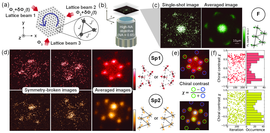
First, we describe our experimental setup. A sample was prepared by loading a Bose-Einstein condenstate (BEC) of 87Rb atoms into a lattice system consisting of an optical triangular lattice and crossed far-off resonance traps (FORT). The optical triangular lattice potential is given by:
| (1) | |||||
where is the lattice depth, the reciprocal lattice vectors, the harmonic trap frequency along the direction perpendicular to the lattice plane, and is the relative phase between two of the three lattice beams, for which we choose the wavelength nm. In Eq. 1, we omit the offset term and the influence of the external trap frequencies in the xy-plane for simplicity. Unless otherwise mentioned, the atoms were initially loaded to a lattice depth of , where is the recoil energy, the wave number, the Planck constant divided by , and the mass of 87Rb atom. The Hubbard parameters are Hz, Hz, where are the on-site interaction and the nearest neighbor tunneling, respectively. The external trap frequencies are Hz.
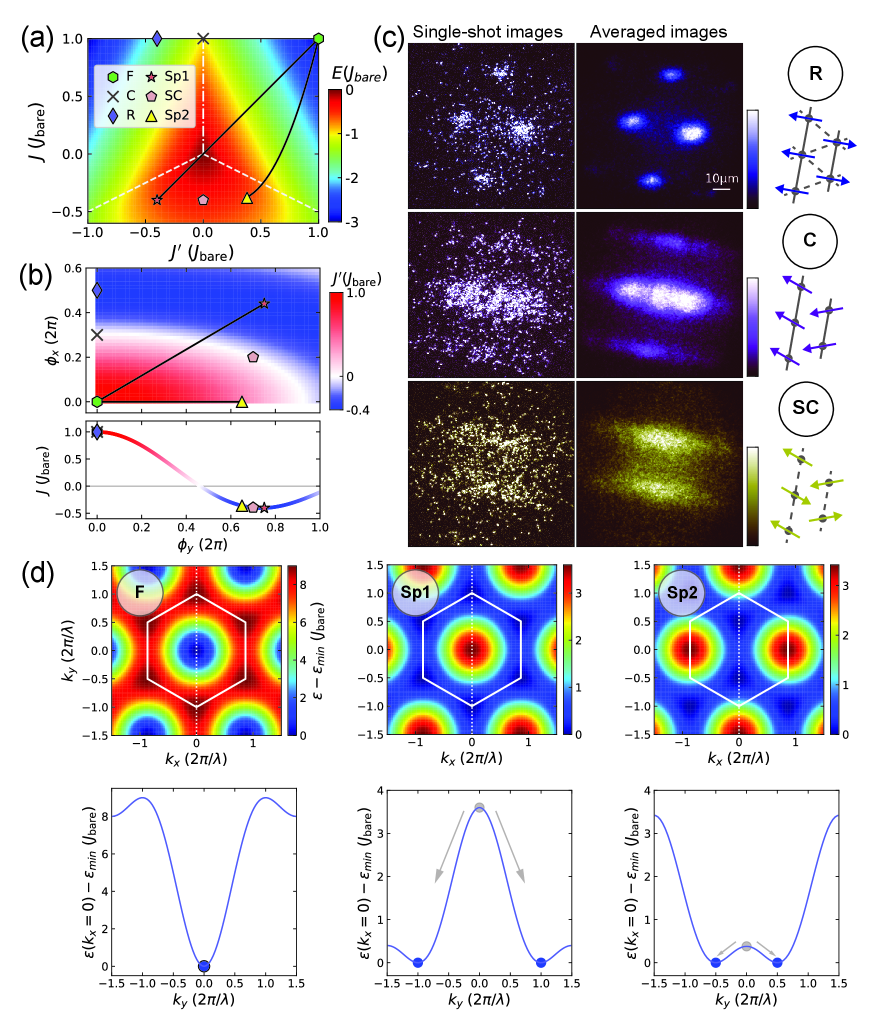
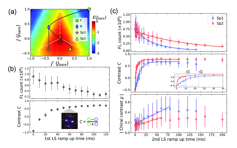
After lattice loading, we increased phase modulation signals to shake the optical triangular lattice elliptically (Fig. 1(a)). According to the Floquet theory, the effective tunnelings and in the rotating frame obey the zeroth order Bessel function of the first kind (see Supplementary Material for the details of lattice shaking parameters and experimental sequence sup ). The effective tunnelings are for Sp1, and for Sp2 throughout this letter. The modulation frequency kHz was carefully chosen to avoid multi-photon interband excitations Weinberg et al. (2015); sup . We also note that the crossed FORTs depths after lattice loading had to be lowered as much as possible so that the evaporation of atoms heated by lattice shaking could work well Reitter et al. (2017); sup . We observed the interference patterns of atoms using in-plane time-of-flight (TOF) Bakr et al. (2010), where the triangular lattice potential was suddenly switched off, whereas the vertical lattice potential was ramped up so that the atomic cloud could expand within the layers. Atoms were typically split into 3 layers in the vertical lattice, and more than 60 of the atoms were populated in a target layer of imaging. The in-plane TOF was followed by (i) a sudden ramp-up of all the optical lattices to freeze out atoms, (ii) selection of the target layer by the combination of microwave and B-field gradient, and (iii) fluorescence imaging using the Raman sideband cooling Yamamoto et al. (2020a). Figures 1(c) and (d) show single-shot and averaged images of atom distributions after 5 ms in-plane TOF. In the case of Sp1 and Sp2, where two-fold chiral degeneracy exists, the symmetry-broken images are observed Struck et al. (2011). We also checked the statistical distribution of the chiral contrast , which is defined in Fig. 1(e). The histograms appear binary, indicating that symmetry breaking often happens. We took the data at a ramp-up time of 200 ms for Sp1 and 300 ms for Sp2 with crossed FORT depth optimized for each frustrated phase sup . The atom number per tube in the shaken lattice differed in each phase because the loss rate during lattice shaking depends on the phase modulation amplitudes. For example, in Sp2, the filling was . Since , this experiment is conducted in the weak interaction regime, where the system is mapped to the classical XY model Eckardt et al. (2010).
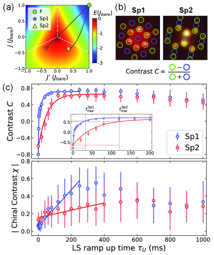
In the following, we focus on the relaxation from F to Sp1 and Sp2 (see Fig. 2(a)). To quantify the relaxation times, we introduce contrast defined in Fig. 2(b). When , the system is in an F state. indicates a phase transition to Sp1 or Sp2. Figure 2(c) shows and with various ramp-up times of the phase modulation signals. The relaxation time of Sp1 is much shorter than that of Sp2. We made a fit to the data of with our empirical exponential functions
| (4) |
where are fitting parameters. We define the rise time such that is satisfied. The extracted rise times are ms, ms. We attribute this difference to two factors; one is the path length ratio after the phase transition over the total length (see black solid lines in Fig. 2(a)). The ratio for Sp1 is 2.6 times larger than that for Sp12. The other is the effective band structures. In the tight-binding approximation, the energy difference between the ground states of Sp1 and point, at which a BEC is populated before lattice shaking, amounts to ; on the other hand, the counterpart of Sp2 is , 9.5 times smaller sup . A BEC at point becomes so unstable in Sp1 that it relaxes quickly into the true ground states. As for , it strongly depends on the crossed FORT depths sup . We note that the offset of in Sp2 data shifts upward since the regions of interest (blue and green circles in Fig. 1(e)) are close to points.
At a short ramp-up time of around 100 ms in Fig. 2(c), is positive, which means that the phase transition has already happened. At the same time, is still small, which indicates that the simultaneous occupation of both chiral modes is observed more often than symmetry-broken images are. In a previous study Struck et al. (2011), the possibility of domain formation was mentioned; however, this has yet to be confirmed. Therefore, we conducted an investigation to clarify this issue. The direct observation of chiral-mode domains in optical lattices was proposed in Kosior and Sacha (2014) assuming the far-field regime, which is difficult to reach in our system since the trap frequency limits in-plane TOF. Instead, we attempt to detect the formation of the chiral domains by observing the interference of spatially separated chiral modes.
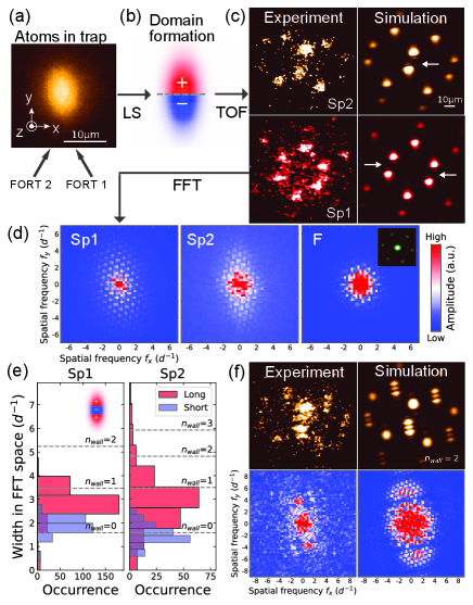
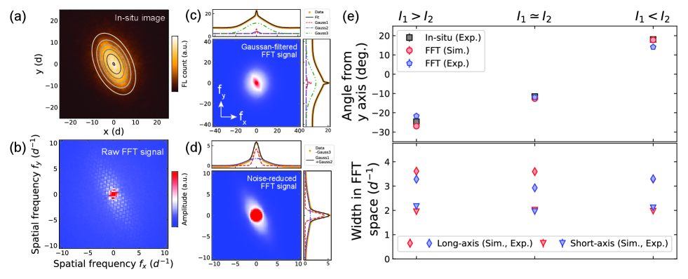
Figure 3(a-c) explains the processes from the domain formation to the observation of interference by the in-plane TOF. As shown in Fig. 3(a), the atoms in the optical triangular lattice and crossed FORTs have a shape elongated along the y-axis. We assumed that during the ramp-up time, a linear domain wall as shown in Fig. 3(b), which is the simplest of its kind, is formed most likely along the x-axis because the domain wall energy is proportional to its length. During in-plane TOF, wave packets with different chiral modes interfere with each other. Consequently, interference fringes are observed. Figure 3(c) shows single-shot images of Sp1 and Sp2 with fringes and simulated images. To visualize the effect of fringes, we applied a fast Fourier transform (FFT) to the TOF images. Figure 3(d) shows the amplitude spectrum of the FFT images averaged over more than 100 runs. The spectrum spreads over along the y-axis, which results from fringes. For comparison, the amplitude spectrum of F without lattice shaking is also shown. It appears symmetric, with no signs of fringes. We made a fit to the FFT signals to extract the widths along the long and short axes sup . Figure 3(e) shows the histograms together with numerical simulation assuming various numbers of domain walls. While a single domain wall is dominant, multiple domain walls are sometimes formed in Sp2. Figure 3(f) shows the experimentally observed TOF image with multiple domain walls and the simulated image with . In the FFT signals, we can see side peaks that result from interference of the same chiral modes.
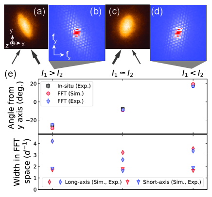
Finally, the orientation of the domain wall was controlled using crossed FORTs. The trap frequencies in the xy-plane are dominated by FORT 1 and FORT 2 (Fig. 3(a)), which have much tighter beam waists of 23 m than the horizontal beam waists of the three beams that comprise the triangular lattice m Yamamoto et al. (2020a). Therefore, the direction along which the atomic cloud is elongated depends on the intensity balance between FORT 1 and FORT 2. Figure 4(a) shows the atom distribution when the intensity of FORT 1, , was much stronger than that of FORT2, . The amplitude spectrum of the FFT in Sp2 is oriented in line with the atom distribution (Fig. 4(b)). Figure 4(c), (d) are the opposite case. Figure 4(e) compares the angles and widths in FFT space at different balances of FORTs. We can see good agreement between experiment and numerical simulation assuming .
In conclusion, we studied the relaxation from the ferromagnetic phase to two frustrated phases (Sp1 and Sp2) in the XY model on shaken optical triangular lattices. We revealed that domain walls Parker et al. (2013); Kock et al. (2015); Wang et al. (2022) are formed in Sp1 and Sp2, which accounts for the simultaneous occupation of the two chiral modes. In this study, the system does not reach a strongly correlated regime. When the interaction is increased to , one can access frustrated quantum magnetism, where the appearance of gapped spin-liquid phases is predicted Eckardt et al. (2010). The system can be mapped onto the spin-1 quantum XY model Altman and Auerbach (2002); Yamamoto et al. (2020b) near the Mott insulating state with unit filling. In this situation, the quantum phase transition between the chiral superfluid and Mott insulator, where the symmetry of U(1) is broken, can be investigated. Non-equilibrium dynamics after quenching across the phase transition and formation of domain structures can reveal the quantum Kibble-Zurek mechanism in this model Keesling et al. (2019).
Acknowledgements.
We thank Daisuke Yamamoto for helpful discussions. This work was supported by JSPS KAKENHI Grant Numbers JP19H01854, 23H01133, ImPACT Programme of Council for Science, Technology and Innovation (Cabinet Office, Government of Japan), and JST ERATO-FS Grant Number JPMJER2204.Supplemental Material for
Observation of Chiral Domain Structures in a Frustrated XY Model on Optical Triangular Lattices
S1 Phase diagram of a frustrated XY model
In a tight-binding approximation, the renormalized dispersion relation in the periodically driven triangular lattice is
| (S1) |
where is the lattice constant. The parabolic dispersion relation term along the direction perpendicular to the triangular lattice plane is omitted. According to the dispersion relation Eq. S1, the minima of energy are given by
| (S6) |
where we assigned the same names as in Struck et al. (2011) to the spin configurations that are realized with the different spin-spin couplings . The corresponding phase at each lattice site is given by:
| (S7) |
where is a lattice vector. Equation S6 does not include the cases for where the system forms decoupled chains and the dispersion relation along becomes degenerate. Energy of dispersion relation at the position of minima is equivalent to the ground state energy of the classical XY model per particle :
| (S10) |
Figure S1(a) shows a zero-temperature phase diagram of the classical XY model in a triangular lattice based on Eq. S10.
The expressions of the phase modulation signals for the triangular lattice beams can be written as
| (S11) | |||||
| (S12) | |||||
| (S13) |
where is the driving frequency, and are the modulation amplitudes. Thus, the effective tunneling processes are expressed as
| (S14) | |||||
| (S15) | |||||
| (S16) | |||||
| (S17) |
where is the zeroth order Bessel function of the first kind. Figure S1(b) plots as a function of . Figure S1(c) shows experimentally observed interference patterns of unfrustrated phases. Figure S1(d) shows the effective band dispersion relations of F, Sp1, and Sp2 based on Eq. S1 using in Fig. S1(a),(b).
S2 Experimental sequence and micromotion effect
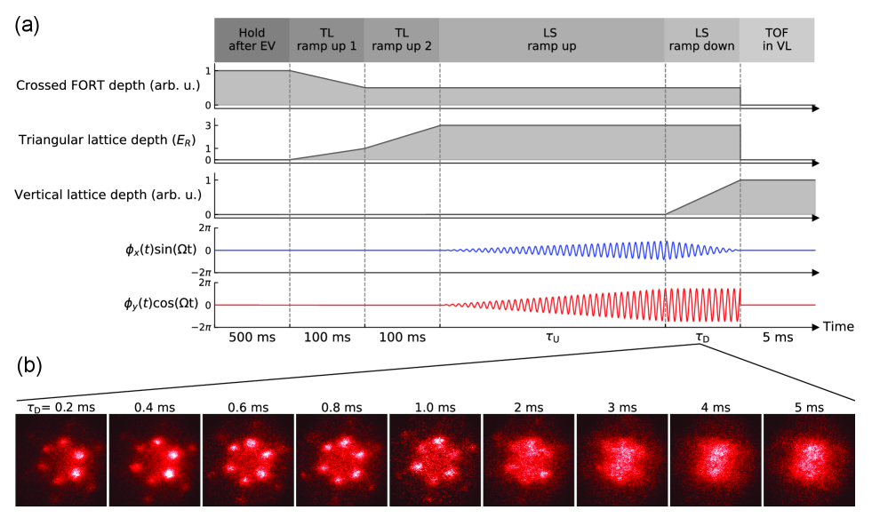
Figure S2 shows the experimental sequence from the holding time of the crossed FORTs after evaporative cooling to in-plane TOF. After 500 ms of holding atoms in the crossed FORTs for thermalization, we ramped up the optical triangular lattice to in 100 ms and simultaneously ramped down the crossed FORTs to a moderate depth so that the Flquet evaporation could efficiently work (see the S.4 Flquet evaporation). In the 2nd ramp of 100 ms, the optical triangular lattice was increased to . Subsequently, the phase modulation amplitudes to drive the positions of the optical triangular lattice were ramped up with various times as in Fig. 2 of the main text. Before the in-plane TOF, the vertical lattice depth increased to nK. Simultaneously, one of the phase modulation signals was decreased to zero to eliminate the micromotion effect that inherently arises in Floquet systems Goldman and Dalibard (2014); Eckardt (2017); Guo et al. (2019). Figure S2(b) displays the in-plane TOF images in Sp1 with several ramp-down times, . In the case of ms, the atoms undergo a momentum kick (i.e., a micromotion) at the end of elliptical modulation of the lattice position. Consequently, the centers of the envelope in the momentum distributions shift. In contrast, if , the elliptical modulation reduces to a liner modulation, where the micromotion can be removed as long as the final phase of the remaining modulation signal is set to fulfill arg. A too long , however, leads to relaxation from Sp1 to Sp2 via Staggered 1D chains (see Fig. S1(b)). We set ms in our experiments.
S3 Multi-photon interband excitation in a driven triangular lattice
In quantum systems with Flquet engineering, the heating effect during the periodic drive is the most serious problem. In the case of driven optical lattices, the major cause of this heating is multi-photon excitation between time-averaged energy bands Arlinghaus and Holthaus (2010); Weinberg et al. (2015). The periodic modulation with frequency causes the interband coupling processes that conserve quasimomentum but change the energy by integer multiples of the photon energy . An -order multi-photon transition is assumed to occur when the following resonance condition is fulfilled:
| (S18) |
where , and is the time-averaged single-particle energy of -th band with quasimomenta .
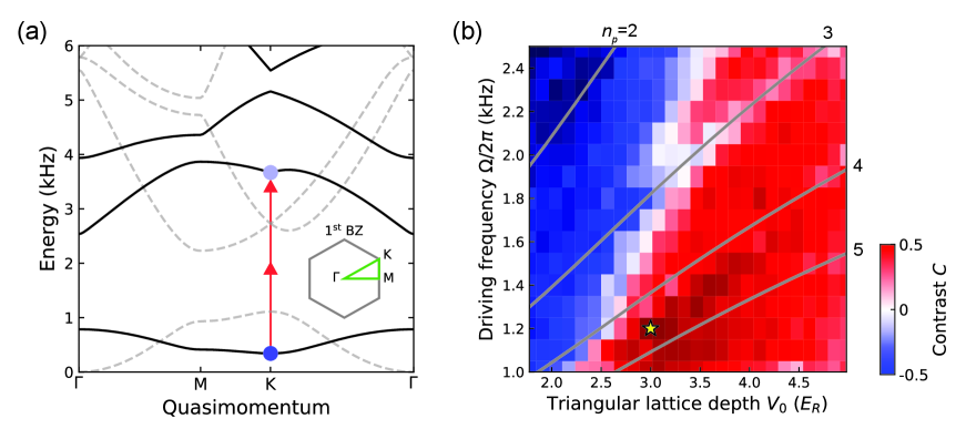
Figure S3(a) shows the effective energy bands of the triangular lattice with in the case of Sp1. The red arrows indicate the two-photon transition from the lowest to the first excited band. These interband transitions caused by periodic driving significantly reduce the contrast defined in Fig. 2(a). The decrease in can be attributed to two distinct processes. First, the atoms excited into higher bands are no longer trapped in the optical lattice. Thus, the atomic losses reduce the bosonic enhancement . Second, an interacting BEC in the excited bands rapidly decays owing to the scattering processes, which results in a decrease in the degree of coherence in the system Martikainen (2011); Paul and Tiesinga (2013).
Figure S3(b) shows the results of a spectroscopic study of these multi-photon transitions in the driven triangular lattice. The excitation spectra were taken with various lattice depths at fixed forcing amplitudes . The resonant driving frequencies in Eq. S18 with different are plotted together with the excitation spectra. These calculations agree with the experimental data, and multi-photon excitations up to the fourth-order are visible, which is consistent with a previous study Weinberg et al. (2015). We note that to keep constant throughout the spectroscopy, the final amplitudes of phase modulation were adjusted according to Eqs. S16, S17. The maximum was reached within a narrow parameter region between and . In the main text, we use and kHz for this reason.
S4 Floquet evaporation
As explained in the previous section, the triangular lattice depth and driving frequency are important parameters to avoid multi-photon interband transitions. Another salient factor that should be considered to reduce heating in Floquet-engineered quantum gases is Floquet evaporation Reitter et al. (2017). As in Fig. S4(a), we found that the crossed FORT depth during the Floquet drive should be decreased such that the resonantly scattered atoms can leave the trap before dissipating their energy into the system. We examined the effect of Floquet evaporation by applying a B-field gradient along the z-axis (Fig. S4(b)). Without the B-field gradient, heated atoms can evaporate because of gravity. When a B-field gradient was applied to cancel the gravity, the atomic ensemble suffered from heating and exhibited no interference peaks. When the B-field gradient was stronger than gravity, the visibility recovered, as expected.
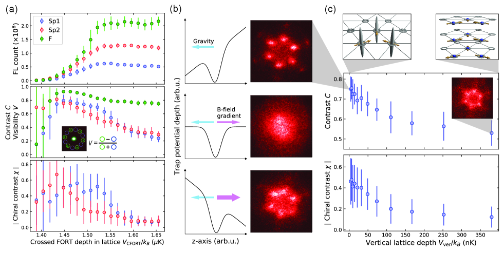
Figure S4(c) shows the dependence of and for Sp1 on the vertical lattice depth in the driven triangular lattice. As increases, both and decrease, which indicates that Floquet evaporation along the z-axis does not work well in the presence of the vertical lattice because it prevents thermal atoms from evaporating along the gravitational direction. This could be a crucial problem for the experimental realization of the strong interaction regime () in the two-dimensional driven lattice systems.
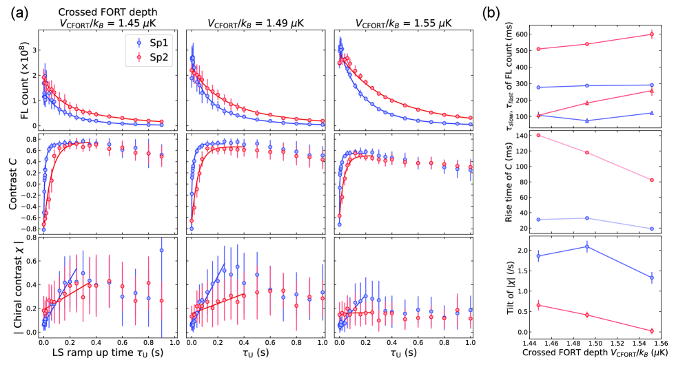
We systematically investigated dependence on the crossed FORT depth and LS ramp-up time. Figure S5(a) shows the results. The contrast and chiral contrast of the middle column in Fig. S5(a) correspond to Fig. 2(c) in the main text. Figure S5(b) summarizes the fitting results. These results and Fig. S4(a) ensure that although the crossed FORT depth affects the maximum values of and , it does not change the fact that the relaxation from F to Sp1 is much faster than that from F to Sp2.
FL count and in Fig. S5(a) are fitted by single or double exponential functions, while is fitted by a linear function with offset. Ideally, might also be fitted by an exponential-like function in the same way as the contrast . In reality, however, the loss and heating of atoms cause both and to decrease in long ramp-up times. Since these loss and heating mechanisms are too complex, we excluded the experimental data of the long ramp-up times from fitting. Unlike , the plateau of , which is important if one wants to make a fit to the data with an exponential-like function, can hardly be seen. Therefore, we approximated the fitting function to a linear one in the case of .
S5 Relaxation from Rhombic to Spiral 1 and Spiral 2
In Fig. 2(c) of the main text, we observed relaxation from F to Sp1 and Sp2. We found that the rise time of contrast differs between Sp1 and Sp2, which we attribute to the length of the path and the effective band structure. To ensure this scenario, we checked relaxation from R to Sp1 and Sp2 as seen in Fig. S6(a), which is the opposite case of relaxation from F to Sp1 and Sp2 used in the main text. Therefore, the relaxation time to Sp2 should be faster than that to Sp1.
We used a two-step ramp-up of the Floquet drive. The first ramp-up is to prepare R as an initial state. Figure S6(b) shows relaxation from F to R with various ramp-up times. We set the first ramp-up time at 60 ms, where atoms already become an R state. In the second ramp-up, atoms relax from R to Sp1 and Sp2. Figure S6(c) shows the results. As expected, the rise time of in Sp1 ms is slower than that in Sp2 ms, which is the opposite case of Fig. 2(c) in the main text. In making a fit to , the definition of the empirical function in Eq. 2 is reversed such as
| (S21) |
The reason why a double-exponential function is used for Sp1 in Eq. 2 and for Sp2 in Eq. S21 is because atoms go through a non-condensate state around the center of the phase diagram. There are two distinct processes; First, the distribution of atoms swiftly spreads in momentum space. Second, the atoms condensate again at a true ground state relatively slowly. FL count in the second ramp-up is fitted by a single exponential function instead of a double exponential function because the initial fast decay has already occurred in the first ramp-up. is fitted by a linear function with offset, the same as in the main text.
S6 Details of fitting to FFT signals
In Fig. 3(e) and Fig. 4(e) of the main text, the angle in images and FFT images and the widths in FFT images are plotted. In this section, we describe how the information was obtained.
As in Fig. S7, the images were fitted by a two-dimensional (2D) elliptic Gaussian function with tilt and offset to know the angles and widths of the atomic distribution before in-plane TOF. The fitting results were used for the numerical simulation of spin domains, the details of which are described in the following section S7.
As for the FFT signals, we extracted the information about angles and widths by using the following triple 2D Gaussian function;
| (S22) | |||||
where are fitting parameters. The first 2D Gaussian (Gauss1) is for the inherent interference pattern of the triangular lattice, the second 2D Gaussian (Gauss2) for the fringes originating from spin domains, and the third 2D Gaussian (Gauss3) for noises in the experimental data. Gauss1 and Gauss2 have the same form. Because of this, although different initial guesses were used for and in making a fit, they were sometimes swapped. So, they were sorted after the fit. Before the fit, we applied a Gaussian filter with to the raw FFT signals, as in Fig. S7(b), to smooth out the spikes of the inherent interference patterns, whose spacing in FFT signal is . Figure S7(c) shows the Gaussian-filtered FFT signal of Sp2 together with the fitting results accumulated along the x-axis or y-axis. Figure S7(d) shows the FFT signals with Gauss3 subtracted to clarify that the experimental data is well fitted by Gauss1 and Gauss2.
Figure 4 in the main text shows the angle and widths of Gauss2 in Eq. S22 using the data of Sp2. We conducted the same analysis on the data of Sp1 and confirmed that the experimental data agree with the numerical simulation, as in Fig. S7(e).
S7 Simulation of spin domains
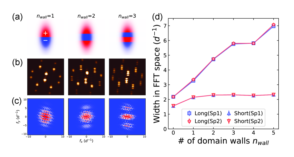
To support our spin domains scenario, we numerically simulated the TOF of samples with spin domains. To simplify the numerical simulation, we assumed that Gaussian-shaped wavefunctions were located at each lattice site. The width of the wavefunction was extracted from the Gaussian fit to the Wannier function in the calculation with a lattice depth . The phases of Sp1 or Sp2 configurations for a homogeneous system were attached to the wavefunctions. We set domain walls perpendicular to the long axis of the elongated initial atom distribution and the opposite chiral modes for each region (Fig. S8(a)). The weight of the wavefunctions was determined by the initial density profile approximated by the 2D elliptic Gaussian function with the tilt angle (Fig. S7(a)). We obtained the density profiles after the TOF of 5 ms by summing all wavefunctions after free expansion. Here, we neglect the effect of residual trapping confinement owing to the vertical lattice.
The simulated density distributions with the number of domain walls from 1 to 3 are presented in Fig. S8(b). In the case of a single domain wall, one can see the effect of the interference between the two chiral modes. When multiple domain walls are formed, on the other hand, interference between the same chiral modes also occurs. We also checked the fast Fourier transformation of the density distributions, as we conducted for the experimental data in the main text, and observed that high-frequency components appeared along the long axis of the initial atom distributions (Fig. S8(c)). To quantify the FFT signals, we made a fit to the data in the same way as is described in the previous section S6. Since the numerical simulation is free from noise, we omitted Gauss3 in Eq. S22. Figure S8(d) shows the extracted widths in FFT space with various numbers of domain walls. The results tell us that the larger the number of domain walls, the larger the aspect of the FFT signals.
References
- H. Diep (2004) H. Diep, Frustrated Spin Systems (World Scientific, Singapore, 2004).
- Moessner and Ramirez (2006) R. Moessner and A. P. Ramirez, Physics Today 59, 24 (2006).
- Balents (2010) L. Balents, Nature 464, 199 (2010).
- Harrison (2004) A. Harrison, Journal of Physics: Condensed Matter 16, S553 (2004).
- Kim et al. (2010) K. Kim, M. S. Chang, S. Korenblit, R. Islam, E. E. Edwards, J. K. Freericks, G. D. Lin, L. M. Duan, and C. Monroe, Nature 465, 590 (2010).
- Qiao et al. (2022) M. Qiao, Z. Cai, Y. Wang, B. Du, N. Jin, W. Chen, P. Wang, C. Luan, E. Gao, X. Sun, H. Tian, J. Zhang, and K. Kim, arXiv:2204.07283 (2022).
- Struck et al. (2011) J. Struck, C. Ölschläger, R. Le Targat, P. Soltan-Panahi, A. Eckardt, M. Lewenstein, P. Windpassinger, and K. Sengstock, Science 333, 996 (2011).
- Mongkolkiattichai et al. (2022) J. Mongkolkiattichai, L. Liu, D. Garwood, J. Yang, and P. Schauss, arXiv:2210.14895 (2022).
- Xu et al. (2023) M. Xu, L. H. Kendrick, A. Kale, Y. Gang, G. Ji, R. T. Scalettar, M. Lebrat, and M. Greiner, Nature (2023), 10.1038/s41586-023-06280-5.
- Lebrat et al. (2023) M. Lebrat, M. Xu, L. H. Kendrick, A. Kale, Y. Gang, P. Seetharaman, I. Morera, E. Khatami, E. Demler, and M. Greiner, arXiv:2308.12269 (2023).
- Prichard et al. (2023) M. L. Prichard, B. M. Spar, I. Morera, E. Demler, Z. Z. Yan, and W. S. Bakr, arXiv:2308.12951 (2023).
- Scholl et al. (2021) P. Scholl, M. Schuler, H. J. Williams, A. A. Eberharter, D. Barredo, K. N. Schymik, V. Lienhard, L. P. Henry, T. C. Lang, T. Lahaye, A. M. Läuchli, and A. Browaeys, Nature 595, 233 (2021).
- Semeghini et al. (2021) G. Semeghini, H. Levine, A. Keesling, S. Ebadi, T. T. Wang, D. Bluvstein, R. Verresen, H. Pichler, M. Kalinowski, R. Samajdar, A. Omran, S. Sachdev, A. Vishwanath, M. Greiner, V. Vuletić, and M. D. Lukin, Science 374, 1242 (2021).
- King et al. (2021) A. D. King, C. Nisoli, E. D. Dahl, G. Poulin-Lamarre, and A. Lopez-Bezanilla, Science 373, 576 (2021).
- Cosmic et al. (2020) R. Cosmic, K. Kawabata, Y. Ashida, H. Ikegami, S. Furukawa, P. Patil, J. M. Taylor, and Y. Nakamura, Physical Review B 102, 094509 (2020).
- Teitel and Jayaprakash (1983) S. Teitel and C. Jayaprakash, Physical Review B 27, 598 (1983).
- Miyashita and Shiba (1984) S. Miyashita and H. Shiba, Journal of the Physical Society of Japan 53, 1145 (1984).
- Lee et al. (1984) D. H. Lee, J. D. Joannopoulos, J. W. Negele, and D. P. Landau, Physical Review Letters 52, 433 (1984).
- Song and Zhang (2022) F. F. Song and G. M. Zhang, Physical Review B 105, 134516 (2022).
- Obuchi and Kawamura (2012) T. Obuchi and H. Kawamura, Journal of the Physical Society of Japan 81, 054003 (2012).
- Lv et al. (2013) J. P. Lv, T. M. Garoni, and Y. Deng, Physical Review B 87, 024108 (2013).
- Eckardt (2017) A. Eckardt, Reviews of Modern Physics 89, 011004 (2017).
- Wang et al. (2009) F. Wang, F. Pollmann, and A. Vishwanath, Physical Review Letters 102, 017203 (2009).
- Jiang et al. (2009) H. C. Jiang, M. Q. Weng, Z. Y. Weng, D. N. Sheng, and L. Balents, Physical Review B 79, 020409(R) (2009).
- Heidarian and Paramekanti (2010) D. Heidarian and A. Paramekanti, Physical Review Letters 104, 015301 (2010).
- (26) See Supplemental Material at [url] for the theoretical and experimental details, which includes Refs. Eckardt (2017); Struck et al. (2011); Goldman and Dalibard (2014); Guo et al. (2019); Arlinghaus and Holthaus (2010); Weinberg et al. (2015); Martikainen (2011); Paul and Tiesinga (2013); Reitter et al. (2017) .
- Weinberg et al. (2015) M. Weinberg, C. Ölschläger, C. Sträter, S. Prelle, A. Eckardt, K. Sengstock, and J. Simonet, Phys. Rev. A 92, 043621 (2015).
- Reitter et al. (2017) M. Reitter, J. Näger, K. Wintersperger, C. Sträter, I. Bloch, A. Eckardt, and U. Schneider, Physical Review Letters 119, 200402 (2017).
- Bakr et al. (2010) W. S. Bakr, A. Peng, M. E. Tai, R. Ma, J. Simon, J. I. Gillen, S. Fölling, L. Pollet, and M. Greiner, Science 329, 547 (2010).
- Yamamoto et al. (2020a) R. Yamamoto, H. Ozawa, D. C. Nak, I. Nakamura, and T. Fukuhara, New Journal of Physics 22, 123028 (2020a).
- Eckardt et al. (2010) A. Eckardt, P. Hauke, P. Soltan-Panahi, C. Becker, K. Sengstock, and M. Lewenstein, Europhysics Letters 89, 10010 (2010).
- Kosior and Sacha (2014) A. Kosior and K. Sacha, Physical Review Letters 112, 45302 (2014).
- Parker et al. (2013) C. V. Parker, L.-C. Ha, and C. Chin, Nature Physics 9, 769 (2013).
- Kock et al. (2015) T. Kock, M. Ölschläger, A. Ewerbeck, W.-M. Huang, L. Mathey, and A. Hemmerich, Physical Review Letters 114, 115301 (2015).
- Wang et al. (2022) X.-Q. Wang, G.-Q. Luo, J.-Y. Liu, G.-H. Huang, Z.-X. Li, C. Wu, A. Hemmerich, and Z.-F. Xu, arXiv:2211.05578 (2022).
- Altman and Auerbach (2002) E. Altman and A. Auerbach, Physical Review Letters 89, 250404 (2002).
- Yamamoto et al. (2020b) D. Yamamoto, T. Fukuhara, and I. Danshita, Communications Physics 3, 56 (2020b).
- Keesling et al. (2019) A. Keesling, A. Omran, H. Levine, H. Bernien, H. Pichler, S. Choi, R. Samajdar, S. Schwartz, P. Silvi, S. Sachdev, P. Zoller, M. Endres, M. Greiner, V. Vuletić, and M. D. Lukin, Nature 568, 207 (2019).
- Goldman and Dalibard (2014) N. Goldman and J. Dalibard, Physical Review X 4, 031027 (2014).
- Guo et al. (2019) X. Guo, W. Zhang, Z. Li, H. Shui, X. Chen, and X. Zhou, Optics Express 27, 27786 (2019).
- Arlinghaus and Holthaus (2010) S. Arlinghaus and M. Holthaus, Physical Review A 81, 063612 (2010).
- Martikainen (2011) J.-P. Martikainen, Physical Review A 83, 013610 (2011).
- Paul and Tiesinga (2013) S. Paul and E. Tiesinga, Physical Review A 88, 033615 (2013).