diagram
Oblique corrections from leptoquarks
Abstract
We present general formulas for the oblique-correction parameters , , , , , and in a model of New Physics having arbitrary numbers of scalar leptoquarks of the five permissible types. We allow for a general mixing among the scalars of the various electric charges, viz. , , , and . We then extend the formulas to the case of a New Physics model with additional scalars in any representations of the gauge group , mixing arbitrarily among themselves.
1 Introduction and notation
Leptoquarks:
In this paper we consider a model of New Physics (NP), i.e. an extension of the Standard Model (SM), that has arbitrary numbers of scalars placed in triplets of colour- which are
-
singlets with weak hypercharge555We use the normalization , where is the weak hypercharge, is the electric charge, and is the third component of weak isospin.
(1) -
singlets with weak hypercharge
(2) -
doublets with weak hypercharge
(3) -
doublets with weak hypercharge
(4) -
triplets with weak hypercharge
(5)
-
the letter denotes singlets of gauge , the letter stands for doublets, and the letter means triplets;
-
the first number in the subscript is two times the third component of weak isospin ;
-
the second number in the subscript is six times the weak hypercharge .
In the notation of the recent Ref. [1], which refers to the original Ref. [2],
-
the scalars in Eq. (1) are leptoquarks of type , viz. scalars placed in the representation of the gauge group ;
-
the scalars in Eq. (2) are leptoquarks of type , viz. scalars placed in the representation of ;
-
the scalars in Eq. (3) are leptoquarks of type , viz. scalars placed in the representation of the gauge group;
-
the scalars in Eq. (4) are leptoquarks of type , viz. scalars placed in the representation ;
-
the scalars in Eq. (5) are leptoquarks of type , viz. scalars placed in the representation of .
Leptoquarks666In this paper we focus exclusively on scalar leptoquarks. Various authors use the term ‘leptoquarks’ to mean some vector, i.e. spin-one, fields. are scalars that are in multiplets of such that they have (renormalizable) Yukawa couplings to one lepton multiplet and one quark multiplet of the SM. Leptoquarks have recently been much used in models that seek to explain one or more unexpected experimental results like those on the muon magnetic moment, the mass, the decays , and the decays ; see for instance Refs. [3, 4, 5, 6, 7, 8, 9, 10].
Oblique parameters:
The oblique parameters are defined as [11]777We use the sign conventions in Ref. [12]. Those conventions differ from the ones used in many other papers, viz. in Ref. [11]. For a resource paper on sign conventions, see Ref. [13]; using the notation of that paper, our convention has and .,888The definitions (6) build on, and generalize, previous work in Refs. [14, 15, 16]. They are appropriate for the case where the functions are not linear in the range . This means that, using those definitions, NP does not need to be much above the Fermi scale.
| (6a) | |||||
| (6b) | |||||
| (6c) | |||||
| (6d) | |||||
| (6e) | |||||
| (6f) | |||||
where is the gauge coupling constant and and are the cosine and the sine, respectively, of the Weinberg angle. The functions are the coefficients of the metric tensor in the vacuum-polarization tensor
| (7) |
between gauge bosons and carrying four-momentum . In
-
one only takes into account the dispersive part—one discards the absorptive part;
-
one subtracts the SM contribution from the full result.999In this paper we do not need to perform this subtraction, since we are dealing with NP scalars that have non-integer electric charges and, therefore, do not mix with the SM scalars.
Note that
| (8) |
has a somewhat simpler expression than .
It is convenient to separate the parameters and in two parts:
| (9) |
The parameters and are identical to the original and , respectively, as they were defined in Ref. [14]:
| (10a) | |||||
| (10b) | |||||
Clearly then,
| (11a) | |||||
| (11b) | |||||
Purpose of this paper:
In this paper we compute the oblique parameters for a NP model with arbitrary numbers of leptoquarks, mixing arbitrarily among themselves. Our work generalizes earlier partial results in Refs. [17, 18, 19, 20, 21, 22]. At the end of this paper we present a generalization wherein the oblique parameters are computed for any NP model solely with extra scalars, whatever the representations of those new scalars are in—just assuming that no new scalar either develops a vacuum expectation value or mixes with the scalars of the SM.
Plan of the paper:
In the next section we write the Lagrangian for the gauge interactions of the scalars, carefully defining the mixing matrices that appear in that Lagrangian. Section 3 performs the computation of the relevant diagrams and explicitly gives various functions that appear in the formulas for the oblique parameters. Those formulas are then given in Section 4. Section 5 presents a few illustrative examples of application of our formulas to simple models with leptoquarks. Section 6 generalizes our work to scalars in any representations of . Section 7 summarizes our main results. In Appendices A and B we deal, respectively, with the counting of mixing parameters and with the parameterization of the mixing in models with leptoquarks. In Appendix C we explicitly demonstrate that and are finite as they should be.
2 Interactions
Numbers of scalars:
There are in our NP model multiplets of type (1), multiplets of type (2), multiplets of type (3), multiplets of type (4), and multiplets of type (5). All these five numbers , , , , and must be multiples of three, since all the scalars are in triplets of ; otherwise, those numbers are free.
Our model has fractionary-charge scalars that we call
-
-type scalars, viz. the ones that have electric charge ;
-
-type scalars, viz. the ones that have electric charge ;
-
-type scalars, viz. the ones that have electric charge ;
-
-type scalars, viz. the ones that have electric charge .
The total numbers of -type scalars, -type scalars, -type scalars, and -type scalars are
| (12a) | |||||
| (12b) | |||||
| (12c) | |||||
| (12d) | |||||
respectively. Notice that
| (13) |
Scalar mixing:
One bi-diagonalizes the leptoquark mass matrices by making
| (14a) | |||||
| (14h) | |||||
| (14o) | |||||
| (14t) | |||||
where in Eq. (14a) stands for a column matrix containing the -type scalars; and analogously for , , and in the other three Eqs. (14). The matrices , , , , , , , , and have dimensions , , , , , , , , and , respectively. The matrices
| (15) |
are unitary.101010Without loss of generality, one may chose a basis where is equal to the unit matrix. We refrain from doing that, in order to keep the notation as general as possible.
Mixing matrices:
We next define the mixing matrices that appear in the charged-current interactions of the scalars. They are
| (16a) | |||||
| (16b) | |||||
| (16c) | |||||
respectively. The factors in Eqs. (16) arise because the charged gauge interactions of the triplets are times stronger than those of the doublets. The mixing matrices that appear in the neutral-current interactions of the scalars are
| (17a) | |||||
| (17b) | |||||
| (17c) | |||||
| (17d) | |||||
where denotes the unit matrix and the matrices , , , and are related to the mixing matrices in Eqs. (16) through
| (18a) | |||||
| (18b) | |||||
| (18c) | |||||
| (18d) | |||||
respectively.
Gauge interactions:
The gauge interactions of the scalars are given by the following pieces of the Lagrangian:
| (19a) | |||||
| (19b) | |||||
| (19c) | |||||
| (19d) | |||||
| (19e) | |||||
| (19f) | |||||
| (19g) | |||||
Notice the presence in Eqs. (19c) and (19d) of the matrices defined in Eqs. (16) and the presence in Eqs. (19e)–(19g) of the matrices defined in Eqs. (17). Also notice that, out of the four matrices in Eq. (19d), only and coincide with matrices in Eqs. (18).
3 Tools for the computation
PV functions:
The Passarino–Veltman (PV) functions [23] and are defined by111111We use the definitions of Ref. [24] for the PV functions.
| (20a) | |||||
| (20b) | |||||
respectively, where is an arbitrary quantity with mass dimension. The quantities , , and are assumed to be non-negative. The PV function in Eq. (20a) is not needed in this paper; on the other hand, we need
| (21a) | |||||
| (21b) | |||||
The PV functions may be numerically evaluated by using softwares like LoopTools [24] and COLLIER [25].121212For the present purposes, in the results given by those codes one should take only the real, viz. dispersive, parts of the PV functions, while dropping the absorptive parts, which have no relevance for the oblique parameters. They may also be evaluated through analytic formulas given in Ref. [26].
The function :
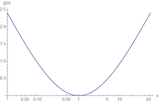
One has [26]
| (22) |
where is a divergent quantity which is defined in Eq. (C3) and cancels out in the final results, and
| (23) |
is a function that obeys and . This function is depicted in Fig. 1.
The function :
The function :
The function :
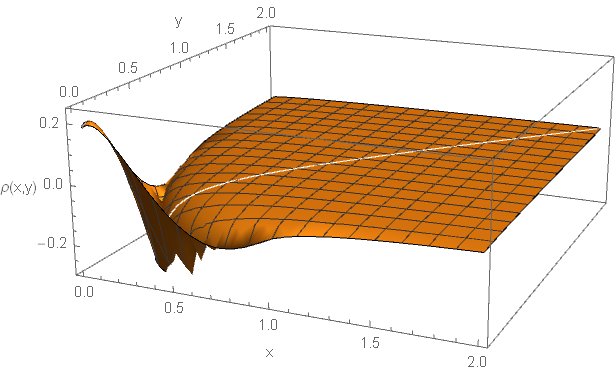
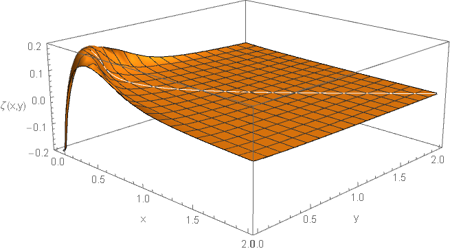
The function —where and are positive—is defined through
| (30) |
which is -independent. Using the analytic formulas in ref. [26] one finds that
| (31) |
The functions and are illustrated in Fig. 2. They are both very small when and .
Computation of the diagrams:
Suppose the vertices and have Feynman rules
| (32a) | ||||
| {fmfgraph*} (75,75) \fmflefti1,i2 \fmfrighto1,o2 \fmfdashesi1,w1 \fmfdashesi2,w1 \fmfphotonw1,o1 \fmfphotonw1,o2 \fmflabeli1 \fmflabeli2 \fmflabelo2 \fmflabelo1 | (32b) | |||
respectively, where and are gauge bosons (v.g. either , , , or ) and and are scalars. Using those Feynman rules we have
| (32ag) |
for diagrams of the form in Fig. 3,
(100,100) \fmflefti1 \fmfrighto1 \fmfboson,label.side=lefti1,w1 \fmfboson,label.side=leftw2,o1 \fmfdashes,right,tension=.3,label=w1,w2 \fmfdashes,left,tension=.3,label=w1,w2 \fmflabeli1 \fmflabelo1
(100,100) \fmflefti1 \fmfrighto1 \fmfboson,label.side=lefti1,w1 \fmfboson,label.side=leftw1,o1 \fmfdashes,label=w1,w1 \fmflabeli1 \fmflabelo1
4 Results for the oblique parameters
:
For the oblique parameter we have
| (32aid) | |||||
where lines (32aid) and (32aid) originate in while lines (32aid) and (32aid) originate in . Utilizing Eq. (24) on Eq. (32ai), we obtain
| (32aj) | |||||
The function is given in Eq. (25). It is a finite function; thus, in Eq. (32aj) there are no divergences, contrary to what happens in Eq. (32ai), wherein the functions and are divergent. The function is moreover positive definite; thus, the two first lines of Eq. (32aj) constitute a positive contribution to , which always exists in a model with leptoquarks, while the two last lines of that equation are a negative contribution, which only exists if at least one of the matrices , , , and has nonzero off-diagonal matrix elements.
and :
For the oblique parameters and we obtain the results
| (32aka) | |||||
| (32akb) | |||||
where the function is given in Eq. (27).
:
and :
Following the decomposition in Eqs. (9)–(11), for the oblique parameters and we have
| (32ama) | |||||
| (32amb) | |||||
where the function is given in Eq. (31); and
| (32ana) | |||||
| (32anb) | |||||
Utilizing Eq. (22), and the cancellation of the divergences proved in Appendix C, one simplifies Eqs. (32an) to
| (32aod) | |||||
| (32aog) | |||||
The function in lines (32aod), (32aod), and (32aog) is given in Eq. (23). In lines (32aod), (32aod), (32aog), and (32aog) is the arbitrary mass introduced in Eqs. (20); and do not depend on the value of , just as they do not depend on the divergent quantity of Eq. (C3).
5 Models with few parameters
We present in this section three examples of leptoquark models, each of them with two leptoquark multiplets and one mixing angle. For the sake of simplicity, for each model we only write down the expressions for the three original oblique parameters , , and . Note that we multiply the original Eqs. (32aj) and (32ao) by a factor 3 because of the three possible colours of each leptoquark.
5.1
There is one -type scalar with mass and there are two -type scalars with masses and . The matrices , , and , where is a mixing angle. Therefore, the matrices , , , and do not exist, , , and . So,
| (32apa) | |||||
| (32apb) | |||||
| (32apc) | |||||
5.2
The is one -type leptoquark with mass , one -type leptoquark with mass , and two up-type leptoquarks with masses and . The matrices , , , , and do not exist; the matrices are just numbers. We have and ; the matrices and do not exist, , and . So,
| (32asa) | |||||
| (32asb) | |||||
5.3
There are one -type leptoquark with mass , two up-type leptoquarks with masses and , respectively, one -type leptoquark with mass , and one -type leptoquark with mass . The matrices , , , and do not exist; the matrices are just numbers, while and . The matrix is a number. Furthermore, , , , and . So,
| (32ava) | |||||
| (32avb) | |||||
| (32avc) | |||||
6 Generalization
In this section we generalize the formulas that we derived for leptoquarks. We consider a set of NP physical scalars with any electric charges, making the provisos that none of the new scalars has vacuum expectation value and that they do not mix with the scalars of the SM. Also, we assume that all the new scalar fields are complex.
We consider a set of physical New Physics scalars that have electric charges (i.e. each has a corresponding ) which differ among themselves by integers.131313If in the NP model under consideration there are physical scalars with electric charges that differ among themselves by non-integer values, then they must be treated separately. For instance, a set of NP scalars with electric charges , , , and (like the leptoquarks) must be treated separately from a set of NP scalars with electric charges , , and . The charges may be either positive or negative.
We place all the scalars of each set in a column vector, ordering the scalars by their decreasing electric charges; this vector generalizes the vector
| (32ba) |
wherein sit the leptoquarks of Section 2.
The column vector of the previous paragraph must constitute a—in general, reducible—representation of the gauge group . Therefore, the following operators, represented by matrices, act on it:
-
1.
The operator , where is the raising operator of the gauge group .
-
2.
The operator , where is the lowering operator of .
-
3.
The Hermitian operator , where is the third generator of .
Since the algebra of has ,
| (32bb) |
The three operators are, of course, represented by matrices that act on the column vector. The matrix is off-diagonal: it only has nonzero matrix elements for . Conversely, the nonzero matrix elements only occur for . The matrix only has nonzero matrix elements when . Since the scalars in the column vector are ordered by decreasing electric charges, one has
| (32bi) |
For instance, in our leptoquark model we had , , and . Clearly then,
| (32bo) |
The electric-charge operator is given in this basis by
| (32bu) |
where the unit matrices have the appropriate dimensions, which may not all be equal. Note that
| (32bv) |
One must also take into account the commutation relation . With and , it yields . Hence, the submatrices in Eq. (32bi) are related by
| (32bwa) | |||||
| (32bwb) | |||||
| (32bwc) | |||||
| (32bwd) | |||||
The gauge-kinetic Lagrangian for the NP scalars is
| (32bxb) | |||||
where
| (32by) |
The Lagrangian (32bx) produces the following interactions of the scalars with the photons:
| (32bza) | |||||
| (32bzb) | |||||
It also produces interactions of the scalars with the gauge bosons, given by
| (32caa) | |||||
| (32cab) | |||||
The interactions of the scalars with the are given by
| (32cba) | |||||
| (32cbb) | |||||
Last but not least, there is the ‘seagull’ interaction of a photon and a with two scalars, given by
| (32cc) |
Therefore,
| (32cda) | |||||
| (32cdb) | |||||
| (32cdc) | |||||
It immediately follows that
| (32ce) | |||||
where we have used . Employing Eq. (24), one obtains
| (32cf) |
One furthermore obtains
| (32cga) | |||||
| (32cgb) | |||||
and
| (32cha) | |||||
| (32chb) | |||||
| (32chc) | |||||
On the other hand,
| (32ci) |
and
| (32cj) |
7 Conclusions
In this paper we have derived general formulas for the oblique parameters in a model with an arbitrary number of scalar leptoquarks. Those formulas include the mixing matrices , , and that appear in the charged current of Eq. (19c); and also the matrices , , , and that are derived from , , and through Eqs. (17) and (18). The final formulas for the oblique parameters are given by Eq. (32aj), and given by Eqs. (32ak), given by Eq. (32al), and and given by Eqs. (32am) and (32ao). The relevant functions , , , and are given by Eqs. (23), (25), (27), and (31), respectively.
We have then considered the more general situation where the New Physics is constituted by (complex) physical scalars that originate in arbitrary representations of the gauge group; those scalars are allowed to freely mix among themselves, but not to mix with the scalar doublet of the SM. In this case the fundamental mixing matrix is that appears in Eq. (32ca); therefrom one derives in Eq. (32bb) and in Eq. (32by). The final results for the oblique parameters are then given in Eqs. (32cf), (32cg), (32ch), and (32cn).
Acknowledgements:
The authors thank the Portuguese Foundation for Science and Technology for support through the projects UIDB/00777/2020, UIDP/00777/2020, and CERN/FIS-PAR/0002/2021. The work of F.A. was furthermore supported by grant UI/BD/153763/2022. The work of L.L. was furthermore supported by project CERN/FIS-PAR/0019/2021.
Appendix A Parameter counting
In our leptoquark models the total number of parameters is . Here,
| (A1) | |||||
is the total number of distinct leptoquark masses; is the number of independent parameters in the mixing matrices. The latter may be computed as follows.
Since the matrices , , , and may be derived fom the matrices , , and through Eqs. (17) and (18), in order to know one must count the parameters in the latter matrices. They are derived from , , , , , , and through Eqs. (16). Let us assume, for the sake of simplicity, the latter matrices to be real. We use the fact that the first rows of an real orthogonal matrix may be parameterized by parameters. Therefore,
| has | (A2a) | ||||
| has | (A2e) | ||||
| has | (A2h) | ||||
| has | (A2i) | ||||
However, one must take into account the fact that, in Eqs. (16), the transformations
| (A3a) | |||
| (A3b) | |||
| (A3c) | |||
where , , and are arbitrary , , and real orthogonal matrices, respectively, leave , , and invariant. Therefore the total number of parameters in , , and is
| (A4) | |||||
Utilizing both Eqs. (A1) and (A4), we find that the leptoquark models with the smallest numbers of parameters are the ones in Table 1.
| 0 | 0 | 1 | 0 | 0 | 1 | 1 | 0 | 0 | 2 | 0 | 2 |
| 0 | 0 | 0 | 1 | 0 | 0 | 1 | 1 | 0 | 2 | 0 | 2 |
| 0 | 0 | 0 | 0 | 1 | 0 | 1 | 1 | 1 | 3 | 0 | 3 |
| 1 | 0 | 1 | 0 | 0 | 1 | 1 | 1 | 0 | 3 | 0 | 3 |
| 0 | 1 | 1 | 0 | 0 | 1 | 1 | 0 | 1 | 3 | 0 | 3 |
| 0 | 1 | 0 | 1 | 0 | 0 | 1 | 1 | 1 | 3 | 0 | 3 |
| 1 | 0 | 0 | 1 | 0 | 0 | 1 | 2 | 0 | 3 | 1 | 4 |
| 2 | 0 | 1 | 0 | 0 | 1 | 1 | 2 | 0 | 4 | 0 | 4 |
| 0 | 2 | 1 | 0 | 0 | 1 | 1 | 0 | 2 | 4 | 0 | 4 |
| 1 | 1 | 1 | 0 | 0 | 1 | 1 | 1 | 1 | 4 | 0 | 4 |
| 0 | 2 | 0 | 1 | 0 | 0 | 1 | 1 | 2 | 4 | 0 | 4 |
| 0 | 1 | 0 | 0 | 1 | 0 | 1 | 1 | 2 | 4 | 1 | 5 |
| 1 | 0 | 0 | 0 | 1 | 0 | 1 | 2 | 1 | 4 | 1 | 5 |
| 0 | 0 | 1 | 1 | 0 | 1 | 2 | 1 | 0 | 4 | 1 | 5 |
| 1 | 1 | 0 | 1 | 0 | 0 | 1 | 2 | 1 | 4 | 1 | 5 |
| 0 | 0 | 2 | 0 | 0 | 2 | 2 | 0 | 0 | 4 | 1 | 5 |
| 0 | 0 | 0 | 2 | 0 | 0 | 2 | 2 | 0 | 4 | 1 | 5 |
| 3 | 0 | 1 | 0 | 0 | 1 | 1 | 3 | 0 | 5 | 0 | 5 |
| 0 | 3 | 1 | 0 | 0 | 1 | 1 | 0 | 3 | 5 | 0 | 5 |
| 2 | 1 | 1 | 0 | 0 | 1 | 1 | 2 | 1 | 5 | 0 | 5 |
| 1 | 2 | 1 | 0 | 0 | 1 | 1 | 1 | 2 | 5 | 0 | 5 |
| 0 | 3 | 0 | 1 | 0 | 0 | 1 | 1 | 3 | 5 | 0 | 5 |
Appendix B Parameterization of the mixing
One may choose to parameterize the mixing matrices in the following way:
-
1.
One sets .
-
2.
One leaves the matrix
(B4) fully free, i.e. with all its parameters.
-
3.
One parameterizes the matrix
(B7) through rotations among the rows of followed by rotations between the rows of and the ones of . For instance, if , one parameterizes the matrix (B7) as .
-
4.
One parameterizes the matrix
(B11) through rotations between the rows of and the ones of , followed by rotations between the rows of and the ones of and by rotations between the rows of and the ones of . For instance, if and , one parameterizes the matrix (B11) as .
Appendix C Cancellation of the divergences in and
Because of Eqs. (14),
| (C1a) | |||||
| (C1b) | |||||
| (C1c) | |||||
| (C1d) | |||||
| (C1e) | |||||
| (C1f) | |||||
| (C1g) | |||||
Using Eqs. (16) and the unitarity of the matrices in Eq. (15), the matrices (18) may be rewritten
| (C2a) | |||||
| (C2b) | |||||
| (C2c) | |||||
| (C2d) | |||||
Divergences:
When , the quantity
| (C3) |
diverges. In Eq. (C3), is Euler’s constant. The PV function
| (C4) |
Therefore,
| (C5a) | |||||
| (C5b) | |||||
divergence:
divergence:
References
- [1] A. Crivellin and L. Schnell, Complete Lagragian and set of Feynman rules for scalar leptoquarks. Comput. Phys. Commun. 271, 108188 (2022).
- [2] W. Buchmüller, R. Rückl, and D. Wyler, Leptoquarks in lepton–quark collisions. Phys. Lett. B 191, 442 (1987) [Erratum: Phys. Lett. B 448, 320 (1999)].
- [3] A. Angelescu, D. Bečirević, D. A. Faroughy, and O. Sumensari, Single leptoquark solutions to the -physics anomalies. J. High Energ. Phys. 2018, 183 (2018). A. Angelescu, D. Bečirević, D. A. Faroughy, F. Jaffredo, and O. Sumensari, Closing the window on single leptoquark solutions to the -physics anomalies. Phys. Rev. D 104, 055017 (2021).
- [4] D. Bečirević, I. Doršner, S. Fajfer, N. Košnik, and D. A. Faroughy, Scalar leptoquarks from grand unified theories to accommodate the -physics anomalies. Phys. Rev. D 98, 055003 (2018).
- [5] J. Kumar, D. London, and R. Watanabe, Combined explanations of the and anomalies: A general model analysis. Phys. Rev. D 99, 015007 (2019).
- [6] R.-X. Shi, L.-S. Geng, B. Grinstein, S. Jäger, and J. M. Camalich, Revisiting the new-physics interpretation of the data. J. High Energ. Phys. 2019, 65 (2019).
- [7] A. Crivellin, D. Müller, and F. Saturnino, Flavor phenomenology of the leptoquark singlet–triplet model. J. High Energ. Phys. 2020, 20 (2020).
- [8] P. Athron, C. Balázs, D. H. J. Jacob, W. Kotlarski, D. Stöckinger, and H. Stöckinger-Kim, New physics explanations of in light of the FNAL muon measurement. J. High Energ. Phys. 2021, 80 (2021).
- [9] A. Bhaskar, A. A. Madathil, T. Mandal, and S. Mitra, Combined explanation of -mass, muon , and anomalies in a singlet–triplet scalar leptoquark model. Phys. Rev. D 106, 015009 (2022).
- [10] P. Athron, A. Fowlie, C.-T. Lu, L. Wu, and Y. Wu, Hadronic uncertainties versus new physics for the boson mass and Muon anomalies. Nature Commun. 14, 659 (2023).
- [11] I. Maksymyk, C. P. Burgess, and D. London, Beyond , , and . Phys. Rev. D 50, 529 (1994).
- [12] G. C. Branco, L. Lavoura, and J. P. Silva, CP Violation (Clarendon Press, Oxford, 1999).
- [13] J. C. Romão and J. P. Silva, A resource for signs and Feynman diagrams of the Standard Model. Int. J. Mod. Phys. A 27, 1230025 (2012).
- [14] M. E. Peskin and T. Takeuchi, New constraint on a strongly interacting Higgs sector. Phys. Rev. Lett. 65, 964 (1990). M. E. Peskin and T. Takeuchi, Estimation of oblique electroweak corrections. Phys. Rev. D 46, 381 (1992).
- [15] G. Altarelli and R. Barbieri, Vacuum polarization effects of new physics on electroweak processes. Phys. Lett. B 253, 161 (1991). G. Altarelli, R. Barbieri, and S. Jadach, Toward a model-independent analysis of electroweak data. Nucl. Phys. B 369, 3 (1992) [Erratum: Nucl. Phys. B 376, 444 (1992)].
- [16] G. Bhattacharyya, S. Banerjee, and P. Roy, Oblique electroweak corrections and new physics. Phys. Rev. D 45, R729 (1992) [Erratum: Phys. Rev. D 46, 3215 (1992)].
- [17] E. Keith and E. Ma, Oblique and Parameters and Leptoquark Models of the HERA Events. Phys. Rev. Lett. 79, 4318 (1997).
- [18] P. H. Frampton and M. Harada, Constraints from precision electroweak data on leptoquarks and bileptons. Phys. Rev. D 58, 095013 (1998).
- [19] A. Crivellin, D. Müller, and F. Saturnino, Leptoquarks in oblique corrections and Higgs signal strength: status and prospects. J. High Energ. Phys. 2020, 94 (2020).
- [20] V. Gherardi, New Physics hints from flavour. E-print 2111.00285 [hep-ph].
- [21] S.-P. He, A leptoquark and vector-like quark extended model for the simultaneous explanation of the boson mass and muon anomalies. Chin. Phys. C 47, 043102 (2023).
- [22] J. Wu, D. Huang, and C.-Q. Geng, -boson mass anomaly from a general scalar multiplet. E-print 2212.14553 [hep-ph].
- [23] G. Passarino and M. J. G. Veltman, One-loop corrections for annihilation into in the Weinberg model. Nucl. Phys. B 160, 151 (1979).
- [24] T. Hahn, Automatic loop calculations with FeynArts, FormCalc, and LoopTools. Nucl. Phys. B Proc. Suppl. 89, 231 (2000). T. Hahn and M. Rauch, News from FormCalc and LoopTools. Nucl. Phys. B Proc. Suppl. 157, 236 (2006).
- [25] L. Hofer, A. Denner, and S. Dittmaier, COLLIER — A fortran-library for one-loop integrals. PoS LL2014, 071 (2014). A. Denner, S. Dittmaier, and L. Hofer, COLLIER: A fortran-based complex one-loop library in extended regularizations. Comput. Phys. Commun. 212, 220 (2017).
- [26] F. Albergaria, L. Lavoura, and J. C. Romão, Oblique corrections from triplet quarks. J. High Energ. Phys. 2023, 031 (2023).
- [27] L. Lavoura and J. P. Silva, Oblique corrections from vectorlike singlet and doublet quarks. Phys. Rev. D 47, 2046 (1993).