Numerically Stable Dynamic Bicycle Model for Discrete-time Control
Abstract
Dynamic/kinematic model is of great significance in decision and control of intelligent vehicles. However, due to the singularity of dynamic models at low speed, kinematic models have been the only choice under many driving scenarios. This paper presents a discrete dynamic bicycle model feasible at any low speed utilizing the concept of backward Euler method. We further give a sufficient condition, based on which the numerical stability is proved. Simulation verifies that (1) the proposed model is numerically stable while the forward-Euler discretized dynamic model diverges; (2) the model reduces forecast error by up to 49% compared to the kinematic model. As far as we know, it is the first time that a dynamic bicycle model is qualified for urban driving scenarios involving stop-and-go tasks.
I Introduction
Model, especially one meets these requirements: simplicity, differentiability, nonsingularity, numerical stability, is widely used in sensing, decision, and control of automated vehicles. For instance, such model describes how the state evolves without noise in an unscented Kalman filter [1], simulates kinematically-feasible trajectories of ego vehicle[2] or surrounding vehicles [3], and forecasts future states in a Model Predictive Controller (MPC) [4]. Moreover, model-based reinforcement learning, such as Approximate Dynamic Programming (ADP), also relies on a state transition model [5].
The modeling of a typical front-steered four-wheel ground vehicle has been developed at various scales. Generally, they can be divided into two categories, i.e., kinematic and dynamic model [6]. Both contain a vast set of models, varying from 1-Degree-of-Freedom (DoF) integrator [7] to 15-DoF full car [8]. This paper focuses on the longitudinal and lateral control of vehicle, which involves 3 DoFs in the planar coordinates. Thus, the simplest model is the 3-DoF bicycle, also known as single-track model.
The two types of bicycle model are applied in different scenarios or tasks. Kinematic model works at low speed, especially stop-and-go scenarios, despite its simplification on tire sideslip characteristics. It is believed to be irreplaceable because all dynamic model encounter a singularity point when approaching zero speed. The tire slip angle estimation term has the vehicle velocity in the denominator [9]. Actually, even at 8 m/s the dynamic model can be unstable (see Fig. 3 (c), forward Euler method). Therefore, though more accurate at certain speeds, dynamic bicycle model can only be adopted when speed is relatively high or the discretization step length is short enough.
An insight into practical control/planning problems requires us to transform the continuous differential kinematic/dynamic bicycle model into a discrete version, i.e. difference equations. Initial Value Problem (IVP) of Ordinary Differential Equations (ODE) is dealt with many mature mathematical techniques, like the Euler method, Runge-Kutta methods, and linear multistep methods [10]. With forward Euler method can be expressed as an explicit linear combination of the derivative , the current state and the step length , which accommodates any form of well. Though less accurate than other explicit methods, it is popular for single-step recurrence. Backward Euler method, one of the implicit methods, usually has better numerical stability but poor computational efficiency, because the next step state has to be approximated by iteration. More importantly, in control-oriented applications like MPC or ADP, the model must have an explicit form of forward propagation, limiting the backward Euler method to offline simulation.
As a result, a kinematic model discretized by forward Euler method is almost the default approach for autonomous parking [11], autonomous intersection management [12] and multi-vehicle formation [13]. However, the modeling error will inevitably grow with driving speed, as tire sideslip angle is no longer negligible.
The rest of this paper is organized as follows. In Section II, both kinematic and dynamic single-track models are illustrated. Section III derives an explicit discrete dynamic bicycle model with due simplifications, which is inspired by the idea of backward Euler method. Further, we manage to give a sufficient condition of provable numerical stability in section IV. The accuracy, stability, computational efficiency as well as support to stop-and-go tasks, are verified in Section V. Section VI gives some concluding remarks.
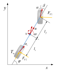
II Bicycle Model
II-A Dynamic Model
The continuous model is given in (1). Here the longitudinal acceleration , where is the longitudinal drive torque from ground, is mass of the vehcle, is the rolling radius of the drive wheel.
| (1) |
where
| (2) |
(a) dynamic, (b) kinematic
The lateral forces , are functions of sideslip angle and . Under mild steering angle, we can assume that
| (3a) | ||||
| (3b) | ||||
| (3c) | ||||
| (3d) | ||||
Note that we use a linear tire sideslip force model here, which is important for the deduction of an explicit discretized form later.
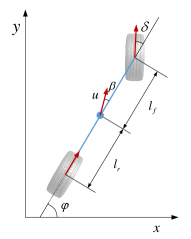
II-B Kinematic Model
The widely used kinematic bicycle model [6] assumes that both front and rear wheels have only longitudinal rolling movement, but no lateral slip. This is inaccurate because tire characteristics are neglected.
| (4) |
where
| (5) |
| (6) |
Note that is longitudinal velocity in dynamic model, and absolute velocity in kinematic model.
III Discretization
To apply the ordinary differential equations (1), (4) to controller modeling or trajectory planning, the foremost step is to solve the initial value problems (IVP) with numerical methods.
As a typical implicit method, the main defect of backward Euler method is that has to be found by solving the rootfinding problem (7), usually using fixed-point iteration.
| (7) |
In order to retain the advantage of explicit methods, we derive in a variable-by-variable fashion. , and are calculated by forward Euler method. and are solved from
Owing to the linear sideslip force assumption, the above formulas have analytical solutions. is special because theoretically, it belongs to a quadratic equation. Therefore, one item, i.e. is simplified into zero. After that, is also derived by forward Euler method. Although such simplification introduces minor modeling error, in a predictive controller, the receding-horizon self-correction will help compensate for possible negative effects.
Technically our discretization is not backward Euler method, but a variant inspired by it. It is the concept of backward Euler method that makes the model stable, which is proved in the next section. The nonlinear discrete model is
| (8) |
which is extended as:
| (9) |
IV Numerical Stability
IV-A linearization of difference equation
The nonlinear recursive difference equation (8) can be linearized around a state point. Firstly, it can be seen as a reference point of the following nonlinear function
| (10) |
it can be derived that
| (11) |
denote as , and as ,
| (12) |
Note that from (11) to (12), the difference item of input was ignored. This is because the input is defined rather than estimated by us. In another word, we do not consider any error originating from .
Additionally, note that the first three state variables, i.e. , and are merely combination and integral of the other variables , and . Thus, we can alternatively consider a dynamic system (still termed for simplicity) with containing only , and , which distinguishes (9) from other systems.
According to the definition of Jacobian matrix, under the reduced system,
| (13) |
| (14) |
| (15) |
IV-B analysis of numerical stability
Our definition of numerical stability is given hereby,
Definition 1
The system described by (9) is called numerically stable if such boundedness characteristic is satisfied:
As a matter of fact, if (12) can be seen as a switched discrete linear system, the concept of Joint Spectral Radius could be of help in the stability proof [14]. However, since the matrix in this case cannot be included by a finite set, we have to seek other methods.
Definition 1 requires that, each entry of the long product does not grow infinity with increasing . This requirement, however, is difficult to be satisfied as the coefficient matrix is varying with each step . More specifically, we believe that the rigorous stability only holds under certain conditions. Therefore, in what follows we manage to give a sufficient condition that will lead to this good feature.
As we have
| (16) | ||||
Thus, the numerical stability will be guaranteed as long as and are both bounded.
IV-B1 boundedness of
The sufficient condition is given as follows.
Condition 1
If Condition 1 is satisfied, the long product will decay exponentially. Moreover, we notice that involves and step length , which means that the norm of will not be an arbitrary value but restricted in a certain range. This physical meaning could be crucial for the establishment of Condition 1.
Proposition 1
is always bounded when approaches infinity, given that Condition 1 is satisfied.
Proof
| (17) | ||||
IV-B2 boundedness of
Proposition 2
is always bounded when approaches infinity, given that Condition 1 is satisfied.
Proof
| (18) | ||||
| (19) | ||||
where
| (20) |
Since the state variables , , are all bounded by their physical meanings, as continuous functions defined over them, and must have maximum values accordingly (20). According to our proof, given that Condition 1 is established, is always bounded by as increases.
Remark 2
The proof is based on linearization of the initial nonlinear difference model. Nevertheless, according to Lagrange’s mean value theorem, the recursive formula (12) can be changed into
| (21) |
And obviously, this will not change the subsequent analysis and conclusion.
Remark 3
Here we give a sufficient instead of sufficient & necessary condition, which means that the violation of Condition 1 does not necessarily bring numerical instability. The main contribution of this condition, is the easy-to-satisfy property (see Fig. 2) under general settings and common speed, which imposes great practical meaning to the application of dynamic bicycle model (9).
V Simulation
As pointed out by Francesco Borrelli et al. [9], a kinematic model has these main advantages: low-speed feasibility and computational efficiency (2015). At the same time, they also observe significant growth of error on the higher speed sinusoidal and winding track tests. Arnaud de La Fortelle et al. [2] then find that is decisive, otherwise error of the kinematic bicycle model will become very large (2017).
Therefore, it is necessary to verify the low-speed feasibility of the proposed model, and compare the differences between both models. In what follows, we choose a vehicle (C-Class, Hatchback 2017) in CarSim as the prototype. Important parameters are listed in Table I. Open-loop simulation is about step steer response, whereas the closed-loop simulation involves a nonlinear MPC controller undertaking a stop-and-go task.
| Parameter | Description | Value |
|---|---|---|
| yaw inertia of vehicle body | 1536.7 kgm2 | |
| front axle equivalent sideslip stiffness | -128916 N/rad | |
| rear axle equivalent sideslip stiffness | -85944 N/rad | |
| distance between C.G. and front axle | 1.06 m | |
| distance between C.G. and rear axle | 1.85 m | |
| mass of the vehicle | 1412 kg | |
| predictive horizon | 20 | |
| control horizon | 1 | |
| discretization step length | 0.1 s |
V-A Open-loop Control
V-A1 backward versus forward
The numerical stability, as well as the insensitivity regarding step length and driving speed, is rather important for autonomous driving application. Before comparison, we first verify if the numerical stability Condition 1 is satisfied. Let 0 m/s 15 m/s, the 2-norm of is shown in Fig. 2. Since , the numerical stability of our model is essentially guaranteed.

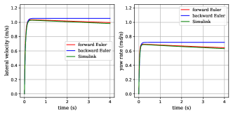
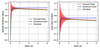
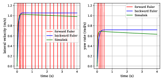
(a) = 0.01 s, (b) = 0.05 s, (c) = 0.1 s
The model (1) with assumptions (3c and 3d) is built in MATLAB/Simulink with 4-order Runge-Kutta solver with a step length of 0.001s. The proposed model shows expected stability over time, and consistency over varying discretization step length (Fig. 3). In contrast, the forward Euler method cannot hold this feature as increases.
V-A2 dynamic versus kinematic
The open-loop step response of dynamic model (discretized by backward Euler method) and kinematic model (discretized by forward Euler method) are calculated, at different velocities. Simultaneously, the same input is imposed on a prototype model in CarSim to approximate the groundtruth.
Prototype: CarSim C-Class, Hatchback 2017
| (m/s) | backward dynamic (m) | forward kinematic (m) | Accuracy Improvement |
| 1 | 0.31 | 0.28 | - |
| 2 | 0.42 | 0.38 | - |
| 3 | 0.37 | 0.36 | - |
| 4 | 0.60 | 0.73 | + |
| 5 | 0.72 | 1.12 | + |
| 6 | 0.93 | 1.72 | + |
| 7 | 1.29 | 2.55 | + |
| 8 | 1.83 | 3.62 | + |
| 9 | 2.62 | 4.98 | + |
| 10 | 3.89 | 6.85 | + |
The open-loop trajectories of both models and their error relative to the prototype in CarSim are shown in Fig. 4.
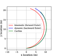
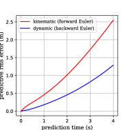
(a) trajectory, (b) location error
Although kinematic model outperforms the backward-discretized dynamic model at lower speeds, this situation is inversed since m/s under defined parameters. To be emphasized, the absolute error at higher speed is much bigger than that of lower speeds. More importantly, the prediction accuracy is crucial at higher speeds where occupants’ lives are at stake.
V-B Closed-loop Control
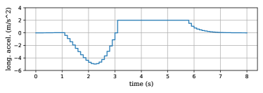
In this section, we design a nonlinear model predictive controller with (9) to comprehensively verify its effect in practical application. Starting from (0,0), the vehicle model is always tracking a direct path connecting its center of gravity (C.G.) and the target (30,30). The reference speed is set to be 6 m/s. There is an obstacle (light blue round area in Fig. 5) located at (15,15) blocking its way. The parameters are deliberately co-designed so that the vehicle can not bypass with steering, but only stop to avoid collision. Note that collision is defined by overlapping of the obstacle and C.G. of the vehicle, instead of vehicle body profile. Once the vehicle stops, the obstacle is moved to (18,12) (dark blue round area in Fig. 5), giving way to the vehicle. Then the vehicle starts to execute a stop-and-go task. To be emphasized, the moved obstacle still requires it to steer and accelerate simultaneously, which is similar to a left-turning maneuver after red light at intersections.

The longitudinal velocity is shown in Fig. 6, whereas the longitudinal input and lateral input are recorded in Fig. 7(a) and (b) respectively.

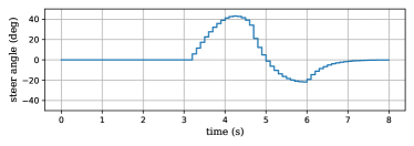
(a) longitudianl input, (b) lateral input
The constrained nonlinear optimal control problem is formulated as (22), satisfying (23).
| (22) |
| (23a) | ||||
| (23b) | ||||
| (23c) | ||||
| (23d) | ||||
is the th reference trajectory point in the predictive horizon, conveys location of the obstacle at th step in the predictive horizon. = diag(100,100,0,0,0,0), = diag(10,500), = diag(1,1,0,0,0,0), = 8. = [-,-,-,0,-4,-3], = [+,+,+,20,4,3]. = [-5,-/4], = [2,/4]. All quantities are in the international system of units.
Our model is computationally efficient as well. The average computation time of one-step MPC solution is 61.6 ms, whereas the same simulation carried out with kinematic model (4) has an average of 59.6 ms. The problem is solved by the nonlinear OCP solver ipopt [15] under the framework CasADi [16], on a laptop with an intel i7 CPU and 12 GB ram.
VI Conclusion
In this paper, we propose a discretized dynamic bicycle model inspired by backward Euler method and a sufficient condition that guarantees its numerical stability. The condition turns out easy to achieve under general vehicle parameters and common urban driving speed (e.g. ). Our method outperforms forward Euler method in stability and shows an advantage in accuracy up to 49% compared to the kinematic model. A comprehensive stop-and-go task further verifies its effectiveness. It could be applied to vast fields, like MPC, ADP, etc., under general urban scenarios.
ACKNOWLEDGMENT
The authors are grateful to Hao Chen and Xuewu Lin for their valuable advice in matrix product derivation.
References
- [1] S. Antonov, A. Fehn, and A. Kugi, “Unscented kalman filter for vehicle state estimation,” Vehicle System Dynamics, vol. 49, no. 9, pp. 1497–1520, 2011.
- [2] P. Polack, F. Altché, B. d’Andréa Novel, and A. de La Fortelle, “The kinematic bicycle model: A consistent model for planning feasible trajectories for autonomous vehicles?” in 2017 IEEE Intelligent Vehicles Symposium (IV). IEEE, 2017, pp. 812–818.
- [3] H. Cui, T. Nguyen, F.-C. Chou, T.-H. Lin, J. Schneider, D. Bradley, and N. Djuric, “Deep kinematic models for physically realistic prediction of vehicle trajectories,” arXiv preprint arXiv:1908.00219, 2019.
- [4] P. Falcone, F. Borrelli, J. Asgari, H. E. Tseng, and D. Hrovat, “Predictive active steering control for autonomous vehicle systems,” IEEE Transactions on control systems technology, vol. 15, no. 3, pp. 566–580, 2007.
- [5] Z. Lin, J. Duan, S. E. Li, H. Ma, and Y. Yin, “Continuous-time finite-horizon adp for automated vehicle controller design with high efficiency,” arXiv preprint arXiv:2007.02070, 2020.
- [6] R. Rajamani, Vehicle dynamics and control. Springer Science & Business Media, 2011.
- [7] Y. Zheng, S. E. Li, J. Wang, D. Cao, and K. Li, “Stability and scalability of homogeneous vehicular platoon: Study on the influence of information flow topologies,” IEEE Transactions on intelligent transportation systems, vol. 17, no. 1, pp. 14–26, 2015.
- [8] M. Perrelli, F. Farroni, F. Timpone, and D. Mundo, “Analysis of tire temperature influence on vehicle dynamic behaviour using a 15 dof lumped-parameter full-car model,” in International Conference on Robotics in Alpe-Adria Danube Region. Springer, 2020, pp. 266–274.
- [9] J. Kong, M. Pfeiffer, G. Schildbach, and F. Borrelli, “Kinematic and dynamic vehicle models for autonomous driving control design,” in 2015 IEEE Intelligent Vehicles Symposium (IV). IEEE, 2015, pp. 1094–1099.
- [10] J. C. Butcher and N. Goodwin, Numerical methods for ordinary differential equations. Wiley Online Library, 2008, vol. 2.
- [11] D. Xu, Y. Shi, and Z. Ji, “Model-free adaptive discrete-time integral sliding-mode-constrained-control for autonomous 4wmv parking systems,” IEEE Transactions on Industrial Electronics, vol. 65, no. 1, pp. 834–843, 2017.
- [12] B. Li, Y. Zhang, Y. Zhang, N. Jia, and Y. Ge, “Near-optimal online motion planning of connected and automated vehicles at a signal-free and lane-free intersection,” in 2018 IEEE Intelligent Vehicles Symposium (IV). IEEE, 2018, pp. 1432–1437.
- [13] M. Cai, Q. Xu, K. Li, and J. Wang, “Multi-lane formation assignment and control for connected vehicles,” in 2019 IEEE Intelligent Vehicles Symposium (IV). IEEE, 2019, pp. 1968–1973.
- [14] R. Jungers, The joint spectral radius: theory and applications. Springer Science & Business Media, 2009, vol. 385.
- [15] A. Wächter and L. T. Biegler, “On the implementation of an interior-point filter line-search algorithm for large-scale nonlinear programming,” Mathematical programming, vol. 106, no. 1, pp. 25–57, 2006.
- [16] J. A. Andersson, J. Gillis, G. Horn, J. B. Rawlings, and M. Diehl, “Casadi: a software framework for nonlinear optimization and optimal control,” Mathematical Programming Computation, vol. 11, no. 1, pp. 1–36, 2019.