Numerical stability analysis of shock-capturing methods for strong shocks I: second-order MUSCL schemes
Abstract
Modern shock-capturing schemes often suffer from numerical shock anomalies if the flow field contains strong shocks, which may limit their further application in hypersonic flow computations. In the current study, we devote our efforts to exploring the primary numerical characteristics and the underlying mechanism of shock instability for second-order finite-volume schemes. To this end, we, for the first time, develop the matrix stability analysis method for the finite-volume MUSCL approach. Such a linearized analysis method allows to investigate the shock instability problem of the finite-volume shock-capturing schemes in a quantitative and efficient manner. Results of the stability analysis demonstrate that the shock stability of second-order scheme is strongly related to the Riemann solver, Mach number, limiter function, numerical shock structure, and computational grid. Unique stability characteristics associated with these factors for second-order methods are revealed quantitatively with the established method. Source location of instability is also clarified by the matrix stability analysis method. Results show that the shock instability originates from the numerical shock structure. Such conclusions pave the way to better understand the shock instability problem and may shed new light on developing more reliable shock-capturing methods for compressible flows with high Mach number.
keywords:
Finite-volume, Shock-capturing, Hypersonic, Shock instability, Matrix stability analysis, MUSCL1 Introduction
Numerical shock prediction is one of the most important issues in computational fluid dynamics, especially for hypersonic flow computations. Shock-capturing methods, based on the mathematical theory of weak solutions, are relatively simple to code and able to simulate any type of flow field, regardless of the presence of shocks [1]. As a result, they are widely used in practical fluid flow simulations. Unfortunately, the computed flowfields involving strong shock waves by modern shock-capturing schemes are often characterized by the appearance of numerical anomalies, such as the carbuncle phenomenon and post-shock oscillations. They frequently arise in hypersonic flow simulations and considerably deteriorate the reliability of the hypersonic heating prediction.
As one of the most famous kinds of shock anomalies, the carbuncle phenomenon was first observed by Peery and Imlay [2] when they computed the supersonic flow field around the blunt-body with the Roe solver. Although the carbuncle phenomenon refers to the spurious solution of blunt-body calculations in which a protuberance grows ahead of the bow shock along the stagnation line [3], it has been generally considered to be a concrete manifestation of numerical shock instabilities. Previous studies have shown that these numerical shock instabilities are more prone to occur in cases where shock-capturing methods own minimal dissipation on discontinuities. Moreover, recent studies [4, 5, 6] even show that dissipative solvers such as the HLLE scheme [7, 8] and the Rusanov scheme [9] (local Lax-Friedrichs), the robustness of which is highly appreciated among experts, are also plagued by the shock instability problem. Thus, although significant progress has been made in numerical methods for compressible flows, it is no exaggeration to say that the modern shock capturing is far away from excellence. During the past three decades, extensive studies have been conducted to clarify the numerical characteristics of the carbuncle phenomenon and propose possible cures for these instabilities. Readers are referred to references [10, 11, 12, 13, 14] and references therein for detailed literature reviews of this subject. Here, we only give a brief account of the persistent efforts to reveal the underlying mechanism of the carbuncle phenomenon, which is the core issue of the current study.
Quirk [3] first performs a comprehensive study of the shock instability problem of approximate Riemann solvers. With the linearized perturbation analysis, he points out that low-dissipative Riemann solvers, such as Roe, add no dissipation on the contact and shear waves in the direction parallel to the shock. As a result, the constant interaction of perturbed pressure and density fields triggers shock instability. Pandolfi and D’Ambrosio [15] extend Quirk’s linearized perturbation analysis to more schemes. They also focus on the relationship between perturbed pressure and density fields and argue that schemes are carbuncle-free if they are able to damp out the density perturbations, such as HLL [7] and van Leer [16]. Gressier and Moschetta [17] employ Quirk’s linearized perturbation analysis and find that the strict stability and exact resolution of contact discontinuities are incompatible. And based on the analysis of the hybrid schemes, Shen et al.[11] find that the third flux component (transverse directional momentum flux component) in the y-direction plays an important role in triggering shock instability. Furthermore, based on the linearized analysis, they reveal that the inconsistent normal momentum distribution along the shock is the source of the shock instability. Simon and Mandal [18, 19] believe that both the mass flux component and interface-normal momentum flux component on the interfaces transverse to the shock front are critical to the shock instability. They investigate the stability of HLLE [7, 8] and HLLC [20] schemes by linearized analysis and numerical experiments and find that the shock instability in the HLLC scheme could be triggered by the unwanted activation of the anti-diffusive term appearing in mass and interface-normal momentum flux component on the interfaces transverse to the shock front. Xie et al.[21] conduct a series of numerical tests with various approximate Riemann solvers and find that the scheme that can preserve the mass flux across the normal shock is shock-stable. Combining the linearized analysis with numerical experiments, they argue that the shock instability can be alleviated if the dissipation corresponding to the momentum is added behind the shock.
In the researches mentioned above, the shock instability is attributed to the insufficient multidimensional dissipation on contact or shear waves. This is consistent with the conclusions of theoretical analysis [22] and physical considerations [23]. However, recent studies by Chen et al.[24, 25] reveal that the inappropriate pressure dissipation of the Riemann solver at the vertical transverse face of a shock is deeply connected to the carbuncle phenomenon and shock instability. Such a useful conclusion is obtained by the stability analysis of a novel shock instability analysis model, which keeps the essential characteristics of numerical shock instability. It also gives support for the partial reasonability of Liou’s conjecture [26], which states that schemes with the mass flux that is independent of the pressure term are not affected by the carbuncle phenomenon. By a linear perturbation analysis, it is found that the pressure dissipation term is equivalent to reducing mass flux perturbations behind shocks, which is found to trigger the shock instability in the view of perturbations [27, 28, 29]. It is noteworthy that Fleischmann et al.[30, 31] attribute the carbuncle phenomenon to the low Mach number problem of Godunov-type schemes. They demonstrate that an excessive acoustic contribution to dissipation in the flux calculation in the transverse direction to the shock front propagation is the prime reason for the numerical instability. The wrong amplitude of pressure fluctuations induced by the low Mach number of the transverse direction will trigger the shock instability. Thus, a fundamentally different approach to stabilize shock-capturing schemes can be achieved by decreasing the viscosity on the acoustic waves for low Mach numbers.
Numerical shock structure is demonstrated to be an important factor that will influence shock instability. Based on the matrix stability analysis, Dumbser et al.[32] and Chauvat et al.[33] find that the shock instability is strongly related to the numerical shock structure. When the internal shock conditions are closer to the upstream states, numerical schemes are more prone to be unstable. These conclusions are validated by the numerical experiments on the 1D and 2D normal shocks from Kitamura et al.[34, 35, 36] and Xie et al.[21]. Moreover, based on the matrix stability analysis, Liu et al.[37] find that there exists a threshold independent of shock strength to trigger instability. According to their work, if the density ratio between both sides of a specific cell interface in the numerical shock structure exceeds a threshold, the computation is unstable. Xie et al.[28] link the shock instability to the inappropriate entropy production inside the numerical shock structure. By dissipation analysis and numerical experiments, they find that if enough entropy production is guaranteed inside shocks, the instability problem can be successfully eliminated. Zaide and Roe [38, 39] investigate the mechanism of numerical shock structure affecting the shock instability and attribute the shock instability to the nonlinearity of the Hugoniot curve. They argue that the intermediate states in the numerical shock structure are always assumed to satisfy the local thermodynamic equilibrium, while this does not hold inside the physical shock, which is the cause of shock instability. Based on their conclusions, Zaide and Roe[40, 41] develop two novel flux functions which can permit stationary shocks with one intermediate state and an unambiguous numerical shock structure and demonstrate their stability.
The computational grid is known as another critical factor that will control the shock instability. Quirk [3] finds that the carbuncle phenomenon will be more pronounced if the grid is aligned to the shock. By the numerical tests, Ohwada et al.[5] reveal that even the robust schemes, such as HLLE [7, 8] and AUSM+ [42], can also yield unstable flow field when the grid is aligned to the shock. Based on a series of numerical experiments, Henderson and Menart [43] conduct a comprehensive study on the effect of the computational grid on the shock anomalies. They find that the aspect ratio of cells near the shock is a factor influencing the magnitude of the carbuncle phenomenon. A larger aspect ratio will yield a more stable flow field. The same conclusion can be found in [5]. Chen et al.[25] also investigate the grid dependence of the shock instability through the matrix stability analysis method. They find that the instability may arise from the transverse face when it is perpendicular to the shock wave, and the shock anomalies may be cured by increasing the angle between the transverse face and the shock front.
It should be noted that Dumbser et al.[32] propose the matrix stability analysis method, coupling the capacity of schemes to stably capture shocks with the eigenvalues of the stability matrix. Based on the matrix stability analysis method, the evolution of perturbation errors can be quantitatively analyzed and easily implemented by programming. Moreover, such an analysis method allows to incorporate the features of the numerical shock, effects of the computational grid, and boundary conditions [18]. As a result, the matrix stability analysis method becomes a powerful tool for judging whether a scheme is stable or not. When the stability analysis yields an unstable result for a scheme, the instability in Euler computations can always be found, although the unstable phenomenon may only appear in certain conditions[11]. Consequently, the matrix stability analysis method is widely used to investigate the mechanism of the shock instabilities [32, 33, 25, 37] and validate the shock stability of the novel shock-stable schemes [24, 44, 45, 46, 47, 48]. However, the matrix stability analysis method proposed in [32] is only applicable to the first-order scheme. Since second or even high-order schemes are actually applied in practical hypersonic flow computations, the shock stability of such methods needs to be investigated in a comprehensive manner. Results from numerical experiments [26, 49] reveal that the stability of the second-order scheme may differ from the first-order case and the limiter used in the second-order scheme plays an important role in triggering the shock instability. Tu et al.[50] and Jiang et al.[51] even investigate the stability of high-order schemes by various numerical experiments and reveal that high-order schemes are at a higher risk of shock instability. However, Kemm[52] thinks that increasing the order offers an alternative way to stabilize the shock position by introducing more degrees of freedom to remodel the Rankine–Hugoniot condition at a captured shock. From the researches above, it can be found that there is no consensus about the influence of spatial order and despite these examples of progress, few efforts have been devoted to analyzing the shock stability of second or even high-order shock-capturing methods quantitatively. Such a situation is mainly due to the lack of an effective analytical method. In the current study, we develop the matrix stability analysis method for the finite-volume MUSCL approach, providing a quantitative analysis tool for the stability of second-order schemes. A follow-up study will present the matrix stability analysis method for high-order finite-volume schemes. The primary numerical characteristics and the underlying mechanism of shock instability for finite-volume schemes can be investigated in detail.
The outline of the rest of this paper is as follows. In section 2, governing equations of compressible flows and their related finite volume discretization are presented. In section 3, the planar steady shock problem is introduced and its associated instability behaviors are presented. In section 4, we establish the matrix stability analysis method for the second-order finite-volume method. Numerical characteristics and the underlying mechanism of shock instability for second-order finite-volume schemes are explored with the developed analysis method in section 5. Section 6 contains conclusions and an outlook on future developments.
2 Governing equations and finite-volume discretization
2.1 The Euler equations
We consider a compressible flow governed by the two-dimensional Euler equations written in integral form as
| (1) |
where denotes boundaries of the control volume and is the flux component normal to the boundary . The vectors of conservative variables and flux are given respectively by
| (2) |
where , , and represent density, specific total energy, and pressure respectively, and is the flow velocity. The directed velocity, , is the component of velocity acting in the direction, where is the outward unit vector normal to the surface element . The equation of state is in the form
| (3) |
where is the specific heat ratio.
2.2 The finite-volume MUSCL schemes
We consider discretizing the system (1) with a cell-centered finite-volume method over a two-dimensional domain subdivided into some structured quadrilateral cells. A particular control volume is shown in Fig.1, and the semi-discrete finite volume scheme over it can be written as
| (4) |
where denotes the average of U on . is the volume of and stands for the length of the cell interface. The flux is the calculated numerical flux that is supposed to be constant along the individual cell interface. In the current study, approximate Riemann solvers are implemented to determine the numerical flux at each cell interface.
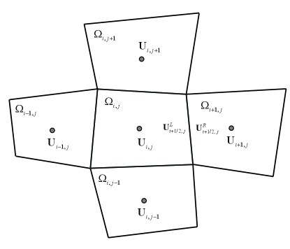
In our study, we devote our efforts to investigating the shock instability of second-order finite-volume schemes, particularly the MUSCL approach [53, 54]. As seen in Fig.1, considering the interface between and , we can get [55, 56]
| (5) |
where and are the variables on the left and right sides of the interface and is called limiter. The limiter is a function of the consecutive gradients, which can be written as
| (6) |
where
| (7) |
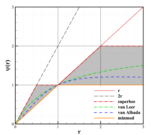
where and are the forward and backward difference operators. When and , and are set to be zero in this paper, respectively. And note that the corresponding scheme becomes first-order accurate if . In the current work, four popular limiters including superbee [57], van Leer [58], van Albada [59], and minmod [60] are employed. Their functions can be written as
| (8) |
As shown in Fig.2, four limiter functions all lie in the shaded region, which is the second-order TVD region [61]. Generally, from the upper boundary of the shadow region to the lower, the limiters become more dissipative [62].
3 The planar steady shock instability
The carbuncle phenomenon is conventionally referred to as the distorted shock ahead of the blunt-body in the supersonic or hypersonic flow [3]. It is essential to choose a simpler test case that shares the fundamental characteristics of the blunt-body carbuncle and can be analyzed simply. In the present work, we consider the 2D steady normal shock problem. It has been well demonstrated that if a scheme yields unstable solutions for the steady normal shock problem, it will also suffer from the blunt-body carbuncle [32, 10, 35].
3.1 Definition of the problem
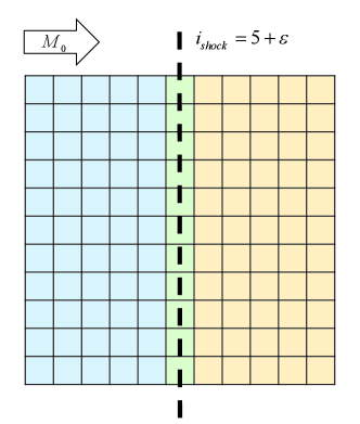
Fig.3 shows the computational grid for the steady shock problem. The initial conditions are prescribed for left () and right () following the Rankine-Hugoniot conditions across the normal shock as
| (9) |
with
| (10) |
where is the upstream Mach number. The intermediate states within the shock () are set according to the Hugoniot curve [33]
| (11) | ||||
with
| (12) |
where is a weighting average that describes the initial state of the internal cell and is called shock position here. The boundary conditions in all directions are imposed through ghost cells. The inflow boundary conditions are set to freestream values, while in order to fix the shock at the same position, the outflow boundary conditions are determined by setting the mass flux at the ghost cells as [35, 63]
| (13) |
Meanwhile, other values are simply extrapolated. The upper and lower boundaries are set as periodic conditions. In order to explore the stability of numerical methods for strong shock capturing, a convergent and stable solution of the 2D planar steady shock problem should be obtained for the linearized stability analysis. Here, the numerical experiment setup presented above is used to carry out numerical tests for the convergent and stable solutions. However, such a convergent and stable flow field is challenging to be obtained, considering that the numerical shock instability may occur in certain cases. In the following section, a simple and effective strategy to enforce a convergent and stable flow field is introduced.
3.2 Initialization of the two-dimensional flow field for stability analysis
In the current study, the 2D flow field for stability analysis is initialized by projecting the steady flow field from 1D computation onto the 2D domain. This initialization method is also employed in [64, 32]. In this way, when a small initial perturbation is introduced into the 2D flow field, it will be damped if the scheme is stable. Otherwise, the initial perturbation will increase, leading to the instability. As a result, we can investigate the stability of different shock-capturing methods by tracking the evolution of the perturbation error. In this paper, the small initial perturbation is set as .
Unfortunately, it has been demonstrated that the shock instability or the carbuncle phenomenon also occurs in the 1D computation. When it happens, the computation fails to converge and a stable solution cannot be obtained. As a result, it is hard to initialize the 2D flow field. The 1D shock instability or carbuncle usually occurs when the Riemann solver that produces stationary discrete shocks with a single interior point is used, such as Roe under the shock position [35, 38, 39, 28]. Xie et al.[21] find that the shock can be stabilized by enforcing the consistency of the mass flux across the normal shock, as a result of which, the stable solution can be obtained. In this paper, this method proposed in [21] is used to obtain a stable result in the 1D domain, which can be written as
| (14) |
where the subscripts and denote the cells just in front of and after the shock structure, respectively. The modification (14) is used in this paper for Roe Riemann solver when , if not mentioned specifically.
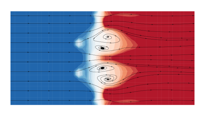
3.3 Carbuncle in 2D steady normal shock problem
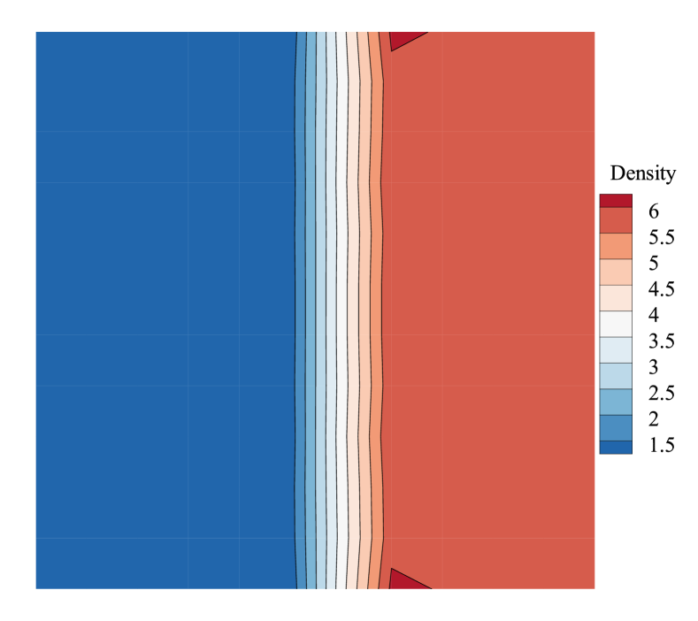
The typical carbuncle phenomenon in 2D steady normal shock problem is shown in Fig.4. As shown, the carbuncle phenomenon is characterized by several convex or concave wedge-shaped shock profiles distributed along the transversal direction in a staggered manner, and vortices appear behind the shock profile [21].
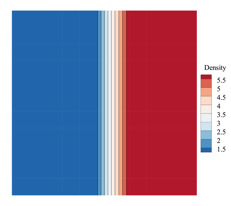
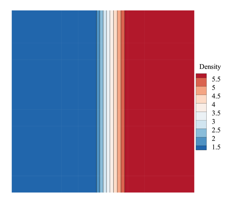
An initial perturbation of size is added on each cell at the beginning of the computation, and Fig.5 shows the evolution of the maximal perturbation error. In the current work, we take the norm of the transverse velocity as the indicator of perturbation error since it is known that the exact solution for mean flows is [32, 43]. Fig.5 and Fig.6 are computed with the condition of and , where the computation is more prone to be unstable. The second-order scheme with Roe solver and van Albada limiter is employed. The computational grid is 1111 Cartesian grid. Third-order TVD Runge Kutta discretization [65] with is used throughout the paper, if not mentioned specifically. As shown in Fig.5, according to the evolution of the perturbation error, there are three stages in the development of the shock instability [32]:
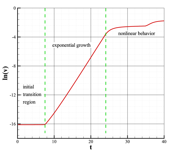
- 1.
-
2.
The evolution of exhibits an exponential increase in the time interval from 7.5 to 24. Thus, this region is called the exponential growth region. The evolution of the perturbation error at this stage satisfies the exponential law
(15) where , , and can be easily obtained from Fig.5, and is called the temporal error growth rate in the present work. The flow field becomes unstable during the exponential growth stage, as shown in Fig.6(b) and Fig.6(c), and the shock profile starts to deform.
-
3.
After time 24, the perturbation error is sufficiently large, nonlinear effects become significant, and the exponential growth is minimized. As seen in Fig.5, the error may fluctuate at a high level during this stage. The flow field, meanwhile, is unphysical. The instability is more severe, as shown in Fig.6(d), and the shock is severely distorted.
As shown in Fig.5, it can be found that the exponential growth stage plays a vital role in the evolution of the perturbation error, determining whether the error will increase or decrease, further stable or unstable, and how quickly it will develop towards instability. Therefore, in the current study we concentrate on the exponential growth stage and relate the shock instability to the temporal error growth rate .
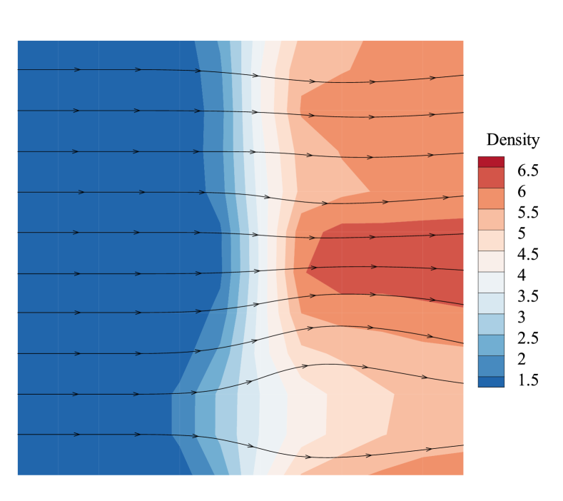
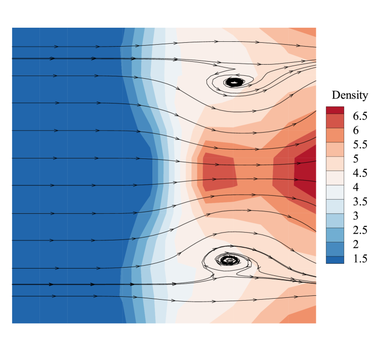
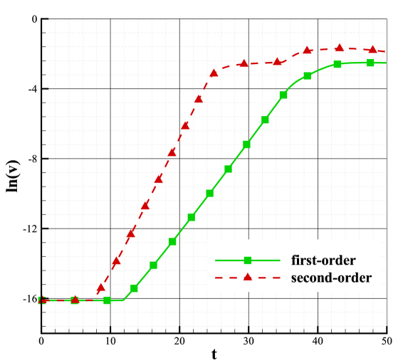
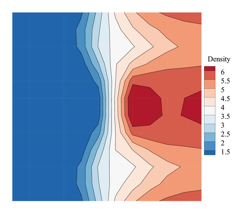
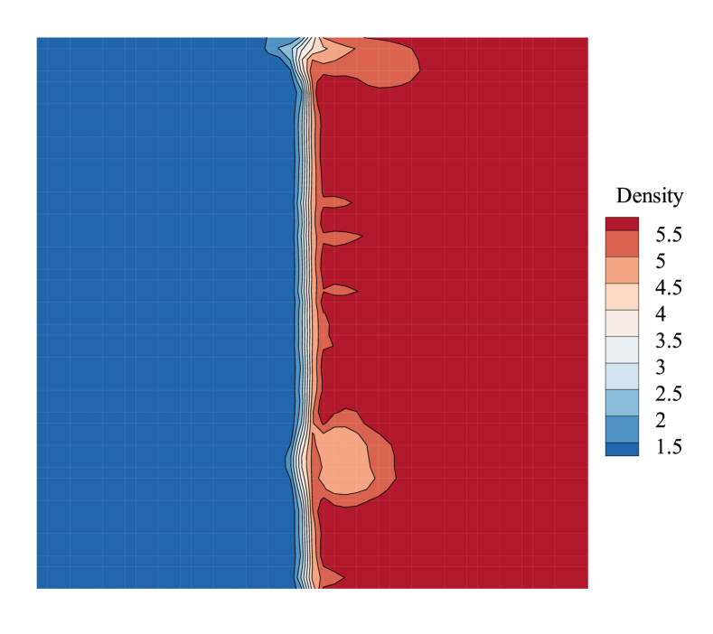
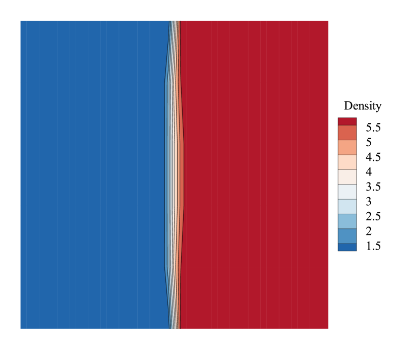
Fig.7 shows the density contours computed by first and second-order schemes at the same computing time. As shown, the shock profile computed by the second-order scheme distorts more severely than the first-order case. And there are vortices appearing behind the shock in the flow field computed by the second-order scheme. Fig.8 is the comparison of the perturbation error, which also shows that the perturbation error produced by the second-order scheme steps into the exponential growth region earlier and increases more quickly. It is also larger at the nonlinear region than that of the first-order scheme. Both Fig.7 and Fig.8 suggest that the shock instability of the second-order scheme is more severe than the first-order scheme. And in the current study, the shock instability of the second-order scheme will be studied in more detail.
4 The matrix stability analysis method for the MUSCL schemes
4.1 The eatablishment of the matrix stability analysis method
The matrix stability analysis method proposed by Dumbser et al.[32] has been well demonstrated to be a useful tool for assessing the shock instability problem of shock-capturing methods. However, such a stability analysis method is only applicable to first-order schemes, which limits its application in analyzing the stability of second and high-order schemes. In the current study, we extend this method for second-order finite-volume schemes, which is presented as follows.
For the stability analysis of a steady field, we assume that
| (16) |
where represents the steady mean value and is small numerical random perturbation. Assume that the random perturbation has no effect on the limiter function. Thus, the limiter is the function of the steady mean value
| (17) |
As a consequence, the matrix stability analysis method can also be applicable for non-differentiable limiters, such as mimod. And the results in section 4 and 5 show that such assumption is appropriate. Substituting (16) into (5), we can get
| (18) |
where and are the variables on the left and right sides of the interface between and . E denotes the unit matrix. Since the numerical flux is the function of and , can be linearized around the steady mean value as
| (19) |
To make the expression brief, the following variables are introduced
| (20) |
Then (19) can be written as
| (21) |
Substituting (16) and (21) into (4) and taking into account that the mean-field is steady, finally, we finally get the linear error evolution mode
| (22) |
where
| (23) |
It can be found from (22) that the evolution of perturbation error in is influenced by the errors in cell itself, four neighbors, and four sub-adjacent cells. However, for the first-order scheme, only the errors in and four neighbors will affect the evolution of the error in [32]. The difference in the linear error evolution model suggests that the shock stability of the first and second-order schemes may be significantly different.
Equation (22) holds for all cells in the computational domain and we finally get the error evolution of all cells in the computational domain
| (24) |
where S is called the stability matrix in the present study. When considering the evolution of the initial error only, (24) can be solved analytically. The solution is
| (25) |
and will remain bounded if the maximal real part of the eigenvalues of S is negative. So the stability criterion is
| (26) |
One should note that equation (19) is accurate only when the numerical flux is differentiable at the mean value, which is not always holding, for example, when the Roe solver is employed and the shock is exactly between two cells (). In the current work, the cases that have numerical shock structure () are analyzed. As a result, the numerical flux calculated by the solvers used in this paper is differentiable at the mean value. The gradients of the numerical flux functions such as can be calculated by the centered difference approximation [11]
| (27) |
where is unit vector of which the component is 1, and [32, 11].
4.2 The primitive variables form of the matrix stability analysis method
It is known that the second-order MUSCL approach (5) can be performed not only in conservative variables but also in primitive variables. The reconstruction of primitive variables is widely used in flow simulation, especially in hypersonic flow simulation, due to its lower cost and broad applicability [66, 67]. Therefore, the matrix stability analysis method in the form of primitive variables is pursued in the current study. The numerical flux is also the function of the primitive variables
| (28) |
where is the vector of primitive variables. Then the flux function can be linearized as
| (29) |
where the variables and in (29) are as follows
| (30) |
Substituting (16) and (29) into (4), we can get
| (31) |
where and are computed by (23). And is the transformation matrix between the conservative variables and the primitive variables. It can be written as
| (32) |
Equation (31) is the primitive variables form of linear error evolution model in . (24) can also be written in primitive variables form as follows
| (33) |
Considering the evolution of initial errors only, the solution of (33) is
| (34) |
And the stability criterion can be seen in (26).
4.3 Quantitative validation of the stability theory
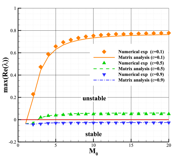
In section 4.1 and 4.2, we introduce the matrix stability analysis method for the second-order MUSCL scheme. By analyzing (25), we can find the maximal real part of the eigenvalues can describe the exponential growth of the perturbation error, which is in (15). Since can be obtained easily by numerical experiments, the reliability of the matrix stability analysis method can be quantitatively verified by comparing and .
The second-order scheme with Roe solver and van Albada limiter is used to perform the quantitative validation. The conditions are and . The computational grid is Cartesian grid. Fig.9 provides the comparison between and , which shows a good agreement between them in both unstable region and stable region. One should note that good agreements can also be obtained by other second-order schemes with different Riemann solvers, limiter functions, and computational conditions. That confirms the reliability of the matrix stability analysis method developed in the current study.
5 Stability analysis of the MUSCL schemes
It is well demonstrated that the shock instability is influenced by a variety of factors, such as Riemann solvers, shock intensity, grid distribution, grid aspect ratio, numerical shock structure, and so on [35, 50, 44, 43]. Numerous numerical experiments are used to investigate how these factors relate to shock instability [35, 21, 43, 50, 68, 5]. The matrix stability analysis method connects the shock stability with the eigenvalues of the stability matrix, making it a quantitative tool for investigating shock stability. With this method, Dumbser et al.[32] and Chen et al.[24, 25] investigate the stability characteristics associated with these factors for the first-order scheme. How will these factors affect the stability of the second-order scheme? In this section, we will answer this question using the matrix stability analysis method established in section 4.
5.1 Stability analysis for different Riemann solvers
It has been demonstrated that the Riemann solver plays an important role in triggering the shock instability [32, 35, 21, 68, 3]. In this section, we further investigate the influence of the Riemann solver on shock instability for the second-order scheme. Here, several approximate Riemann solvers with different dissipative characteristics are considered, including Roe [69, 70], HLL [7], HLLC [20], AUSM+ [42], and van Leer [16]. Note that in this paper, the HLL and HLLC Riemann solvers employ the wave speeds estimate proposed by Davis [71].
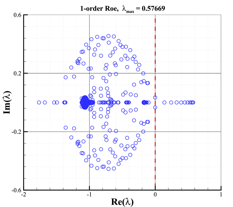
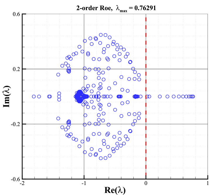
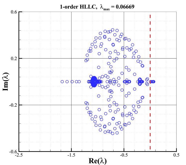
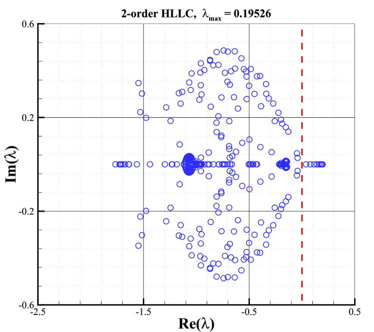
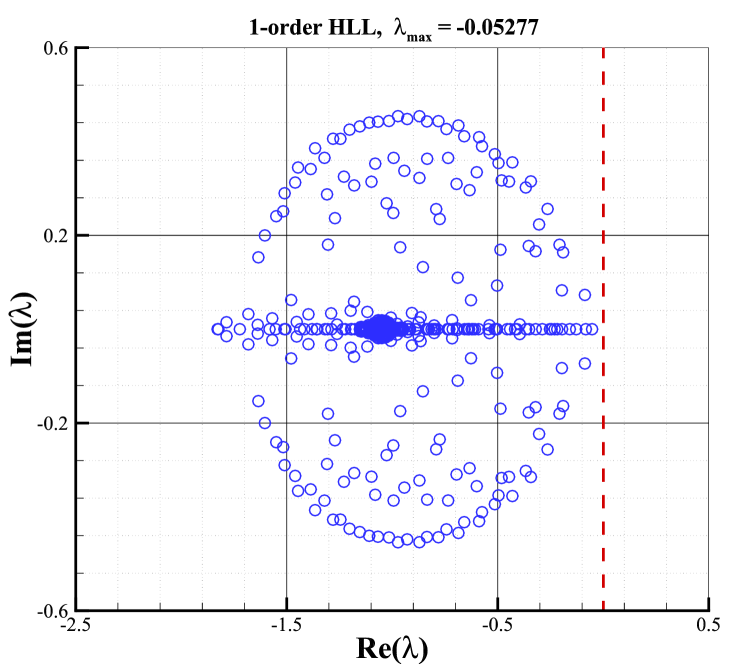
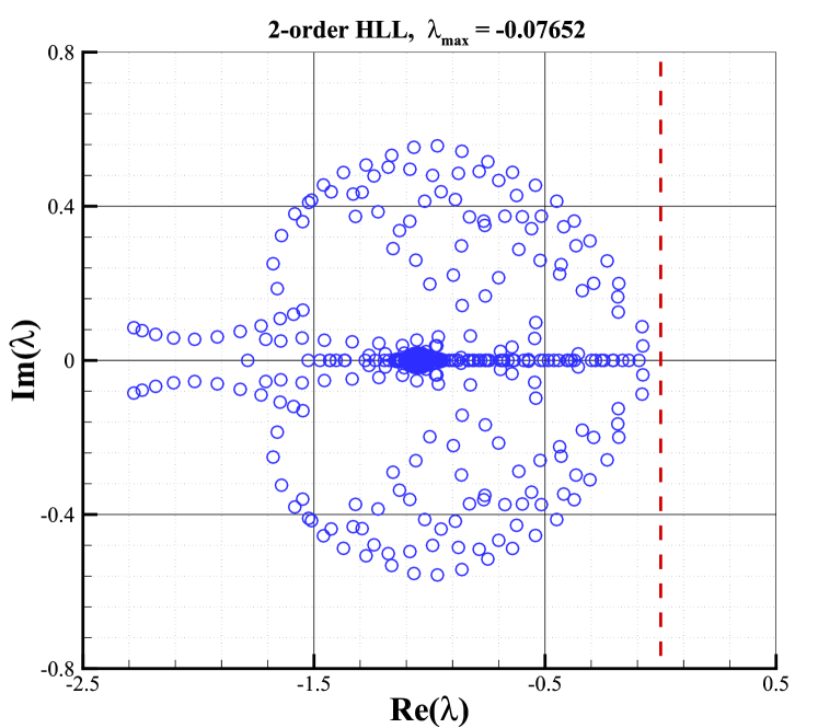
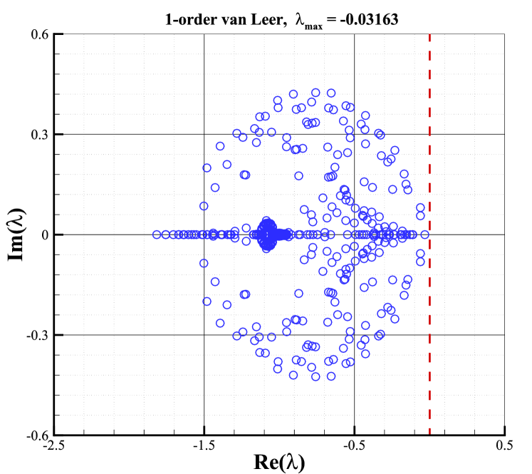
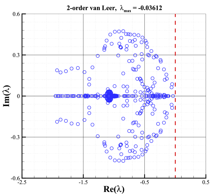
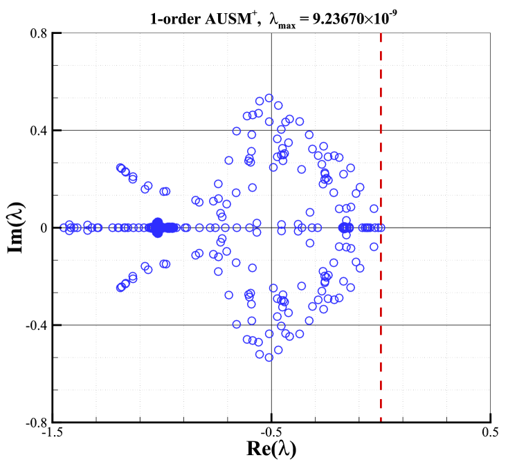
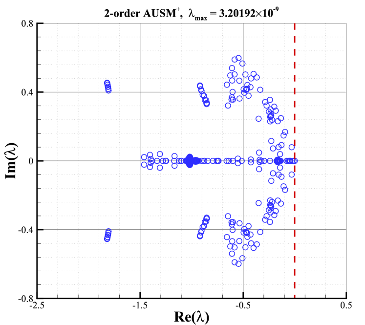
The stability analysis is carried out with the condition of and . All eigenvalues of the stability matrix for the first and second-order schemes with these Riemann solvers are shown in Fig.10. The right column shows the results of second-order schemes with the van Albada limiter, whereas the left column shows the results of first-order ones. According to Fig.10, it can be found that the sign of the maximal real parts of eigenvalues for second-order schemes is closely related to the Riemann solver and is consistent with that of the first-order schemes. It indicates that the Riemann solver still plays a key role in determining the shock stability of second-order schemes as it does for first-order cases. Moreover, As shown, eigenvalues with positive real parts are presented for Roe and HLLC Riemann solvers, which obviously, result in unstable behaviors. It is well-known that both solvers own minimal dissipation on contact and shear waves. On the contrary, the HLL and van Leer Riemann solvers always have eigenvalues with negative real parts, indicating their stability. And both solvers are known as dissipative schemes. What is more interesting is that the maximal real part of the AUSM+ Riemann solver is close to zero, indicating that AUSM+ Riemann solver is marginally stable.
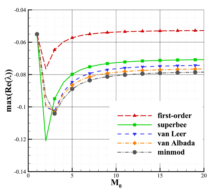
5.2 Influence of spatial accuracy, limiter, and Mach number
To study the influence of spatial accuracy, limiter, and Mach number on shock instability, two typical Riemann solvers, Roe and HLL, are employed in this section. The same investigation can also be conducted on other solvers, such as HLLC, van Leer, and AUSM+, which is not shown for brevity. As seen in Fig.11, the analysis is carried out for the second-order scheme, and in order to investigate the effect of spatial accuracy, results of the first-order scheme are also presented for comparison. Four limiters (superbee, van Leer, van Albada, and minmod) are employed when considering second-order accuracy. By analyzing the results in Fig.11, the following conclusions can be obtained:
-
1.
As shown in Fig.11, we can find that the spatial accuracy will significantly affect the shock instability. The second-order scheme with Roe solver has a larger maximal real part of the eigenvalues than the first-order scheme, which suggests that the second-order scheme with Roe solver is more prone to be unstable than the first-order scheme. However, the maximal real part of the eigenvalues of the second-order scheme with HLL solver is less than that of the first-order case, indicating that the second-order scheme with the HLL solver is more stable than the first-order scheme. The same conclusion as HLL solver can also be obtained from AUSM+ solver, which is marginally stable as shown in Section 5.1. As a result, we can infer that the stability of the stable and marginally stable schemes will be better as the spatial accuracy is enhanced to second-order, while the stability of the unstable schemes will be poorer.
-
2.
For the second-order scheme, the limiter is a critical factor affecting the shock instability. The second-order scheme has the largest maximal real part of the eigenvalues when employing the superbee limiter with the lowest dissipation, while has the smallest maximal real part when using the minmod limiter with the highest dissipation. This indicates that the computation is more prone to be unstable when employing the limiter with lower dissipation. One exception is the HLL solver when . As shown in Fig.11(b), the second-order scheme with HLL solver is more unstable when using minmod limiter, but it is still stable. Anyway, if there is a need to alleviate the shock instability problem in supersonic and hypersonic flow simulations, the limiter with higher dissipation, such as minmod, is preferred.
-
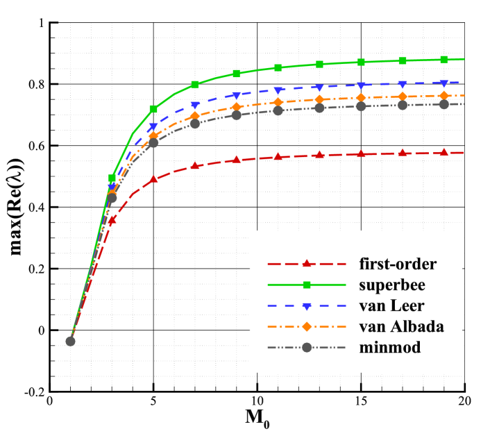
3.
It can be seen from Fig.11 that the Mach number has a significant impact on the shock instability. When the Mach number is modest, the maximal real part of the eigenvalues increases quickly with the increasing Mach number, but when the Mach number is greater than a threshold, the growth will slow down and the maximal real part of the eigenvalues even remains unchanged. The threshold is determined by the Riemann solver, spatial accuracy, and limiter. It implies that when the Mach number is modest, its influence is evident, and the shock instability becomes more severe as the Mach number increases. However, the influence of the Mach number is limited. If the Mach number exceeds a threshold, it will do little to the shock stability. It should also be noted that the scheme with HLL solver is most stable when the Mach number is 2 or 3 (for the first-order scheme and second-order scheme with superbee limiter, the Mach number is 2, and for the others is 3.).
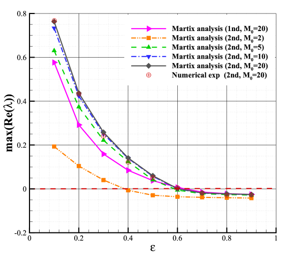
5.3 Analysis of the numerical shock structure
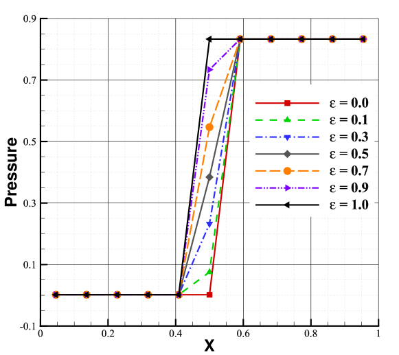
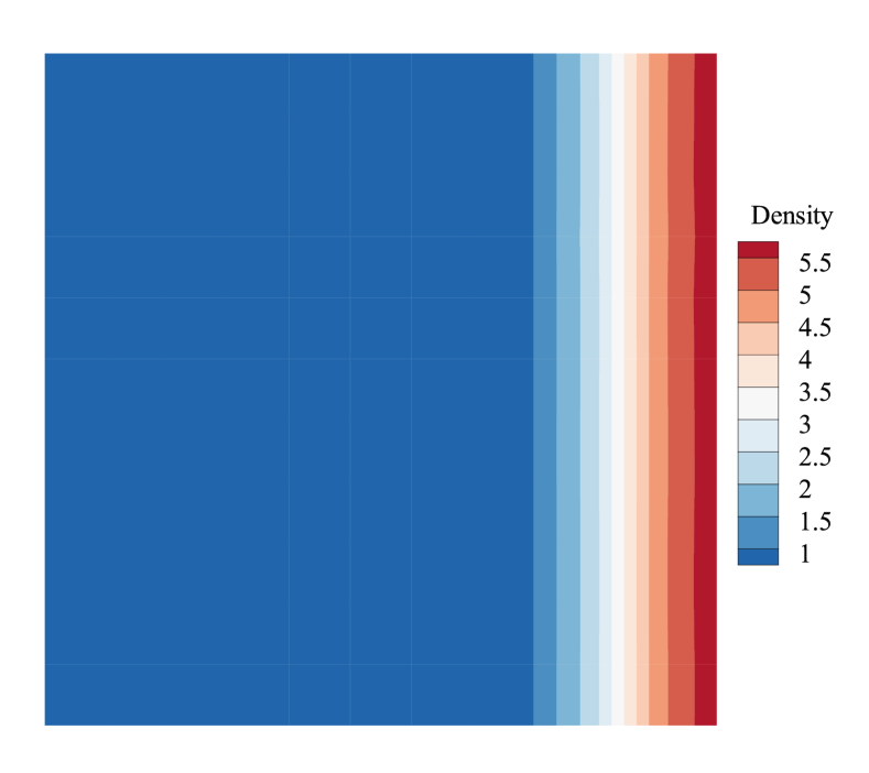
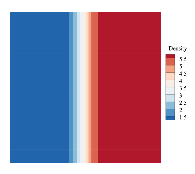
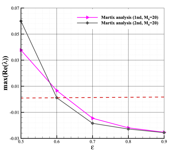
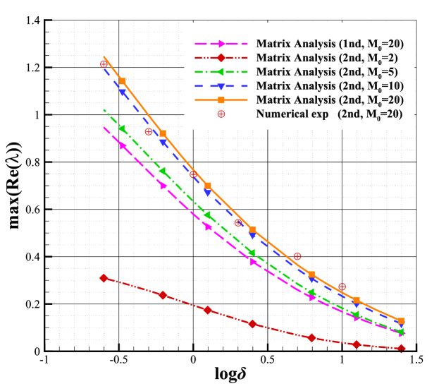
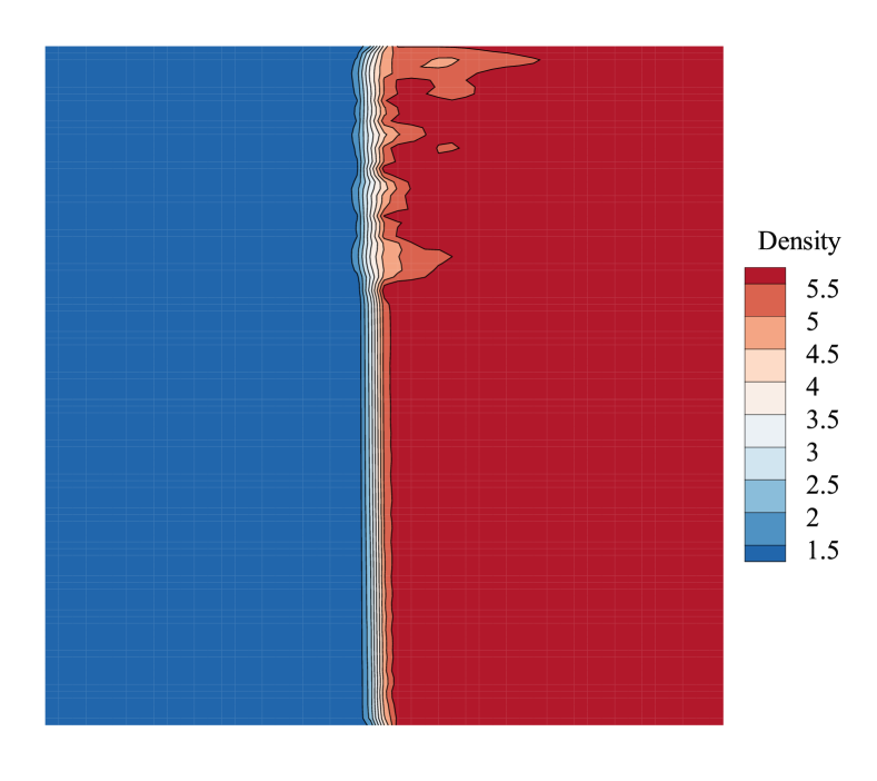
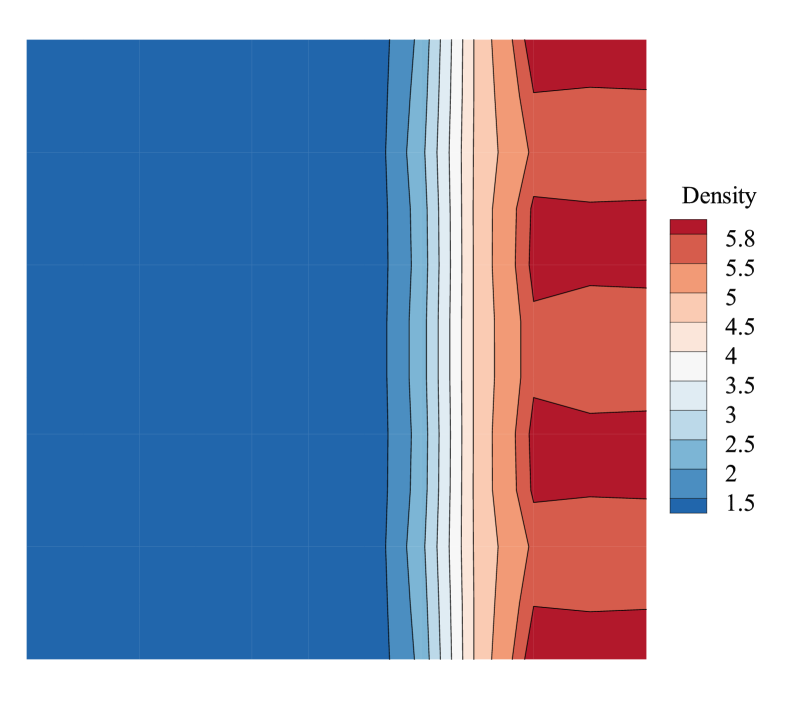
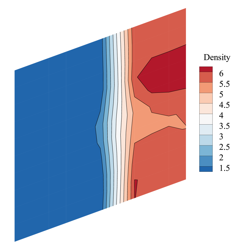
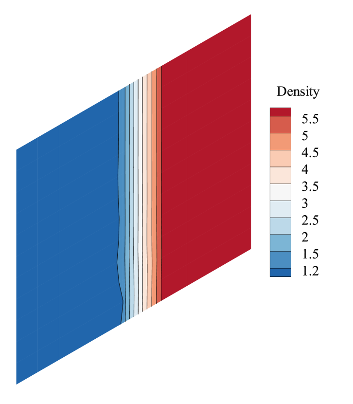
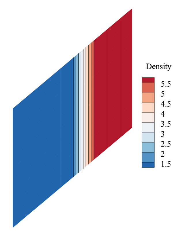
It has been found that the numerical shock structure plays a vital role in shock instability. In this section, we investigate the impact of the numerical shock structure for the second-order scheme using the matrix stability analysis method. Since we are more concerned about the unstable behavior, Roe solver, which is proved to be more prone to be unstable, is employed to perform the remaining analysis. Fig.12 shows the effect of the numerical shock structure. As shown, with increasing, the maximal real part of the eigenvalues of the second-order scheme decreases, and when exceeds a threshold, the maximal real part of the eigenvalues begins to be less than 0. The threshold is related to the Mach number, around 0.4 when and around 0.6 when . Fig.14 is the convergent results of the 1D shock with different . According to Fig.12 and Fig.14, we can conclude that the second-order scheme will be more stable when the internal shock conditions are closer to the downstream states. The density contours with different numerical shock positions are shown in Fig.15, demonstrating the validity of the matrix stability analysis.
Fig.12 also indicates that the numerical shock structure has the same impact on both first and second-order schemes. The unstable scheme can be stable by setting the internal shock conditions closer to the downstream states, whether for the first or second-order schemes. Moreover, When , both the first and second-order schemes with Roe Riemann solver are unstable. And the maximal real part of the eigenvalues of the second-order scheme is greater than that of the first-order scheme, which suggests that the stability of the second-order scheme is worse than the first-order scheme. However, as shown in Fig.12 and Fig.13, when the maximal real parts of the eigenvalues for both first and second-order schemes are less than zero or slightly larger than zero, indicating that the computation is stable or marginally stable. Furthermore, in the region of , the maximal real part of the eigenvalues of the first-order scheme is greater than that of the second-order scheme, suggesting that the stability of the second-order scheme is better than the first-order scheme, which is consistent with the conclusion in Section 5.2.
5.4 Grid dependence of the shock instability
In addition to the influence of the Mach number, spatial accuracy, limiter function, Riemann solver, and the numerical shock structure, the computational grid also plays a significant role in shock instability [43, 5, 15, 32, 25]. In this section, we study further about how the grid affects the stability of the second-order scheme in capturing strong shocks from the perspectives of aspect ratio and distortion angle.
5.4.1 The aspect ratio
In this paper, the aspect ratio can be defined as
| (35) |
where represents the x-direction length of the cell, and is the y-direction length. In the current study, we analyze the case where the computational domain is and . The aspect ratio is then altered by changing the number of cells in the y-direction. Fig.16 shows how the aspect ratio affects the maximal real part of the eigenvalues. According to Fig.16, it can be found that the maximal real part of eigenvalues decreases when increases. Consequently, we may conclude that the shock instability will be alleviated when the grid becomes more elongated in the y-direction, while it will worsen when the grid is refined in the y-direction. The conclusion is validated in Fig.17 by numerical experiments, in which the flow fields become more stable as the aspect ratio increases. Furthermore, it can be inferred from Fig.16 that the aspect ratio has the same effect on the first and second-order schemes: the shock instability can be alleviated by increasing the aspect ratio. And the second-order scheme is always more unstable than the first-order scheme with different aspect ratios under the same Mach number.

The analysis of the aspect ratio offers guidance for us during the grid generation. We can alleviate shock instability by increasing the aspect ratio near the shock, although the effect of increasing the aspect ratio is limited (As shown in Fig.16 and 17, even if the aspect ratio is as large as 10, which may be too large for engineering application, the computation is still unstable.).
5.4.2 The distortion angle
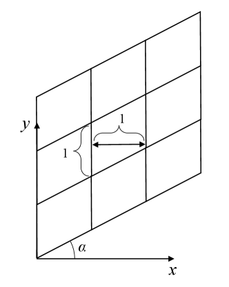
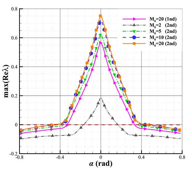
Apart from the aspect ratio, the distortion angle is another factor that could affect the stability of capturing strong shocks [25]. The present work defines the distortion angle as shown in Fig.18. Be aware that is positive when the grid deflects in the counterclockwise direction and negative in the other case. We take in the current work. Fig.19 shows that the maximal real part of the eigenvalues of S is a function of . As shown, for the second-order scheme with the Roe solver, the maximal real part of eigenvalues decreases as increases, and if becomes large enough, it may turn negative. So, the shock instability for the second-order scheme can be cured by increasing the distortion angle of the grid, and the threshold is related to the Mach number. When , the threshold is around , and it will be around if . According to Fig.20, which depicts the flow field with different distortion angles, the shock becomes more stable as the distortion angle increases. It confirms the result of the matrix stability analysis. Note that Zhang et al.[49] find that the carbuncle phenomenon will be eliminated when employing the triangular grid instead of the quadrilateral grid. This may be interpreted by the conclusion here. Moreover, If we compare the differences between the first and second-order schemes, we can find that the maximal real part of eigenvalues of the first-order scheme is always smaller than that of the second-order scheme as the distortion angle increases, whether it will be stable or unstable. As a result, it can be inferred that the stability of the second-order scheme is always worse than that of the first-order scheme as the distortion angle increases.
5.5 Spatial localization of the source of instability
In the above sections, we devote our efforts to exploring the primary numerical characteristics of shock instability for the second-order finite-volume scheme. In this section, we will study further about an important problem about the mechanism underlying the shock instability: spatial localization of the source of instability. Dumbser et al.[32] and Chen et al.[25] investigate this problem and find that the shock instability origins from the upstream of the shock when the shock is resolved exactly between two cells. However, in actual simulation, the captured shock is rarely exactly between two cells. The effect of numerical shock structure is studied by Xie et al.[21]. Based on a series of well-designed numerical experiments, they find that the perturbations inside the shock structure are the main factors to trigger the instability. These studies concentrate on first-order schemes. In this section, we will investigate the spatial localization of the source of instability for the second-order scheme using the matrix stability analysis method.
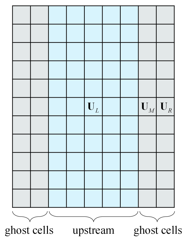
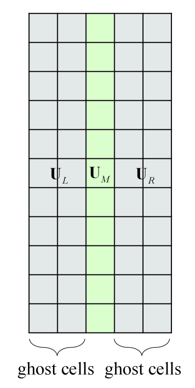
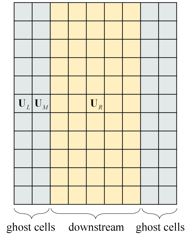
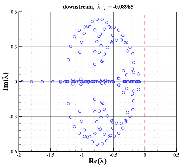
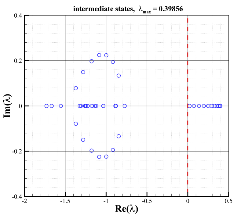
As shown in Fig.21, in order to explore the location of the source of instability, three test cases are employed. In the first one (Fig.21(a)), all cells apart from the ghost cells are set to the upstream state while the right boundary conditions are set to intermediate state and downstream state . Since the boundaries are supposed to be error-free, so their direct contribution to error evolution vanishes in the stability matrix except from the flux-gradient [32]. This procedure prevents any error from developing in numerical shock structure and downstream region, as a result of which we can analyze the stability of the upstream region separately. Identically, in order to analyze the stability of numerical shock structure and downstream region, similar procedures are shown in Fig.21(b) and (c).
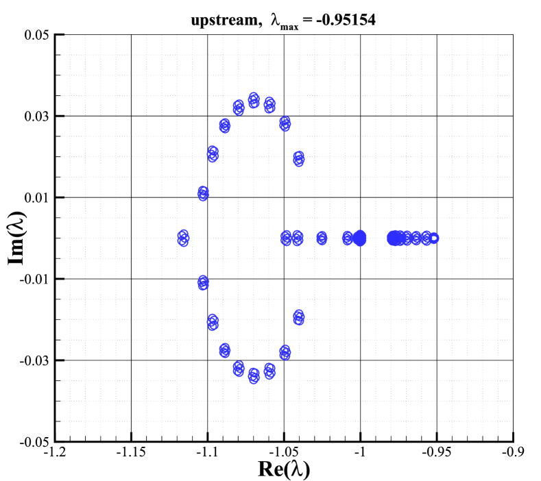
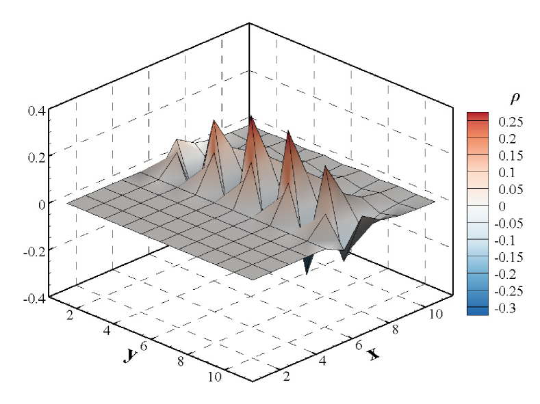
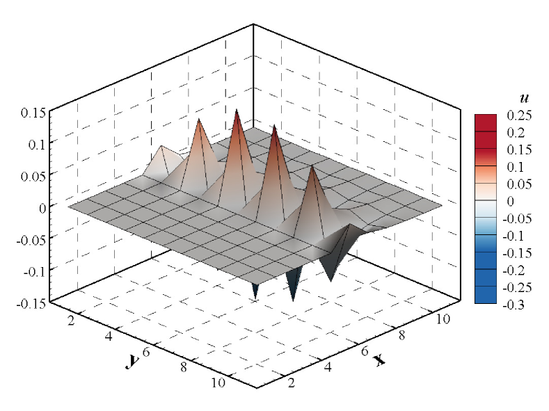
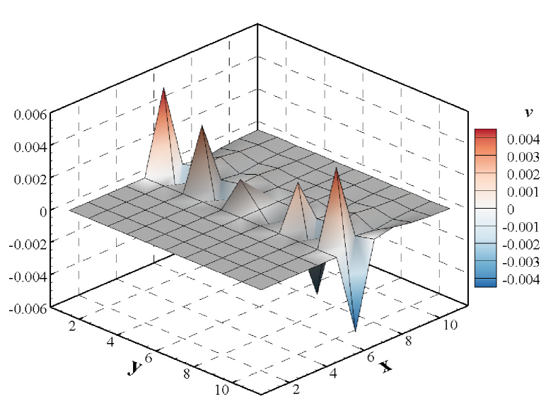
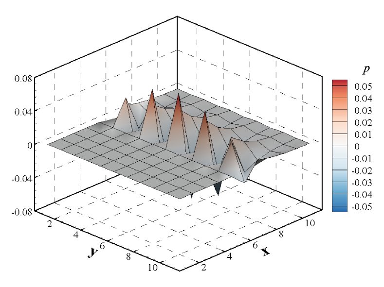
The stabilities of three test cases are investigated using the matrix stability analysis method. Fig.22 shows the distribution of the eigenvalues in the complex plane, from which we can find that the maximal real part of the eigenvalues of the numerical shock structure exceeds 0, while the others are less than 0. As a result, we can infer that in the cases of the shock on the upstream boundary and downstream boundary, the stability analysis predicts a stable behavior, while if the numerical shock structure is contained, the analysis predicts unconditional instability. Moreover, the maximal real part of eigenvalues for the downstream field is larger than that of the upstream field, which may imply that the downstream is more susceptible to being influenced by the unstable information from the numerical shock structure than the upstream. Additionally, the information of the spatial-behavior of the unstable mode is contained in the eigenvectors of the maximal eigenvalue [32]. Fig.23 depicts the unstable mode for the four primitive variables. As shown in Fig.23, the numerical shock structure is the most unstable location, and unstable information will propagate more easily downstream. Thus, according to the analysis in this section, we can conclude that the shock instability originates from the numerical shock structure. And the downstream is more susceptible to being influenced by spurious errors in the shock structure.
6 Conclusion
In this paper, we devote our efforts to quantitatively investigating the shock instability of the second-order scheme. To this end, the matrix stability analysis method for the finite-volume MUSCL approach is developed. With the help of the matrix stability analysis, primary numerical characteristics and the underlying mechanism of shock instability for the second-order scheme are investigated in detail. Results reveal that the shock instability is greatly affected by the shock intensity. The computation for shocks will be more unstable as the Mach number increases. Moreover, the Riemann solver is an important factor affecting the shock stability, whose effect on the second-order scheme is consistent with that of the first-order one. One of the most significant findings to emerge from the current study is that the differences in shock instability between the first and second-order scheme are revealed. When employing high dissipative solvers, e.g. HLL, the stability of capturing strong shocks will be better as the spatial accuracy is enhanced to second-order. However, compared with the first-order scheme, the second-order scheme with low dissipative solvers, such as Roe, is prone to be more unstable. For the second-order scheme, the limiter is demonstrated to be a vital factor in triggering the shock instability. Compared with the low dissipative limiter, the limiter with higher dissipation can decelerate the process towards an unstable result. Except for the factors discussed above, the results have also shown that the computational grid is still a critical element that will significantly affect the shock instability, which will be alleviated by increasing the aspect ratio and distortion angle. Furthermore, the underlying mechanism of the shock instability is still investigated in the current study. And it has been demonstrated that the shock instability originates from the numerical shock structure. The computation for shocks will be more stable when the interval shock conditions are closer to the downstream states.
The current work offers an effective tool to quantitatively analyze the shock stability of the second-order finite-volume MUSCL approach and provides some clues to better understand and control the occurrence of the carbuncle phenomenon or shock instability. However, numerical evidences have shown that high-order schemes are supposed to be at a higher risk of shock instability, and it is more challenging to analyze it in a quantitative manner. Thus, such a quantitative tool that allows to investigate the shock stability of high-order schemes is urgently needed. Corresponding numerical characteristics and the underlying mechanism of high-order shock-capturing methods are more attractive to be investigated in depth. That is what we are addressing now and will be presented in the follow-up work.
Acknowledgements
This work was supported by National Natural Science Foundation of China (Grant No.12202490), Natural Science Foundation of Hunan Province, China (Grant No. 11472004), the Scientific Research Foundation of NUDT (Grant No. ZK21-10), and Postgraduate Scientific Research Innovation Project of Hunan Province (Grant Nos. CX20220010 and CX20220036).
References
- [1] A. Bonfiglioli, R. Paciorri, F. Nasuti, M. Onofri, Moretti’s Shock-Fitting Methods on Structured and Unstructured Meshes, in: Handbook of Numerical Analysis, Vol. 17, Elsevier, 2016, pp. 403–439.
- [2] K. Perry, S. Imlay, Blunt-body flow simulations, in: 24th Joint Propulsion Conference, American Institute of Aeronautics and Astronautics, Boston,MA,U.S.A., 1988, p. 16. doi:10.2514/6.1988-2904.
- [3] J. J. Quirk, A contribution to the great Riemann solver debate, International Journal for Numerical Methods in Fluids 18 (6) (1994) 555–574. doi:10.1002/fld.1650180603.
- [4] K. Kitamura, E. Shima, Y. Nakamura, P. L. Roe, Evaluation of Euler Fluxes for Hypersonic Heating Computations, AIAA Journal 48 (4) (2010) 763–776. doi:10.2514/1.41605.
- [5] T. Ohwada, R. Adachi, K. Xu, J. Luo, On the remedy against shock anomalies in kinetic schemes, Journal of Computational Physics 255 (2013) 106–129. doi:10.1016/j.jcp.2013.07.038.
- [6] T. Ohwada, Y. Shibata, T. Kato, T. Nakamura, A simple, robust and efficient high-order accurate shock-capturing scheme for compressible flows: Towards minimalism, Journal of Computational Physics 362 (2018) 131–162. doi:10.1016/j.jcp.2018.02.019.
- [7] A. Harten, P. D. Lax, B. van Leer, On Upstream Differencing and Godunov-Type Schemes for Hyperbolic Conservation Laws, SIAM Review 25 (1) (1983) 35–61. doi:10.1137/1025002.
- [8] B. Einfeldt, On Godunov-Type Methods for Gas Dynamics, SIAM Journal on Numerical Analysis 25 (2) (1988) 294–318. doi:10.1137/0725021.
- [9] V. Rusanov, The calculation of the interaction of non-stationary shock waves and obstacles, USSR Computational Mathematics and Mathematical Physics 1 (2) (1961) 304–320. doi:10.1016/0041-5553(62)90062-9.
- [10] F. Ismail, Toward a reliable prediction of shocks in hypersonic flow: Resolving carbuncles with entropy and vorticity control., Thesis, University of Michigan (2006).
- [11] Z. Shen, W. Yan, G. Yuan, A Stability Analysis of Hybrid Schemes to Cure Shock Instability, Communications in Computational Physics 15 (5) (2014) 1320–1342. doi:10.4208/cicp.210513.091013a.
- [12] A. V. Rodionov, Artificial viscosity in Godunov-type schemes to cure the carbuncle phenomenon, Journal of Computational Physics 345 (2017) 308–329. doi:10.1016/j.jcp.2017.05.024.
- [13] S. Simon, Numerical Shock Instability In HLL-Based Approximate Riemann Solvers For The Euler System Of Equations: Analysis And Cures, Ph.D. thesis, Indian Institute of Technology Bombay (2019).
- [14] F. Qu, D. Sun, Q. Liu, J. Bai, A Review of Riemann Solvers for Hypersonic Flows, Archives of Computational Methods in Engineering 29 (3) (2022) 1771–1800. doi:10.1007/s11831-021-09655-x.
- [15] M. Pandolfi, D. D’Ambrosio, Numerical Instabilities in Upwind Methods: Analysis and Cures for the “Carbuncle” Phenomenon, Journal of Computational Physics 166 (2) (2001) 271–301. doi:10.1006/jcph.2000.6652.
- [16] B. van Leer, Flux-vector splitting for the Euler equations, in: H. Araki, J. Ehlers, K. Hepp, R. Kippenhahn, H. A. Weidenmüller, J. Zittartz, E. Krause (Eds.), Eighth International Conference on Numerical Methods in Fluid Dynamics, Vol. 170, Springer Berlin Heidelberg, Berlin, Heidelberg, 1982, pp. 507–512.
- [17] J. Gressier, J.-M. Moschetta, Robustness versus accuracy in shock-wave computations, International Journal for Numerical Methods in Fluids 33 (3) (2005) 313–332. doi:10.1002/1097-0363(20000615)33:3<313::aid-fld7>3.0.co;2-e.
- [18] S. Simon, J. Mandal, A cure for numerical shock instability in HLLC Riemann solver using antidiffusion control, Computers & Fluids 174 (2018) 144–166. doi:10.1016/j.compfluid.2018.07.001.
- [19] S. Simon, J. Mandal, Strategies to cure numerical shock instability in the HLLEM Riemann solver, International Journal for Numerical Methods in Fluids 89 (12) (2019) 533–569. doi:10.1002/fld.4710.
- [20] E. F. Toro, M. Spruce, W. Speares, Restoration of the contact surface in the HLL-Riemann solver, Shock Waves 4 (1) (1994) 25–34. doi:10.1007/BF01414629.
- [21] W. Xie, W. Li, H. Li, Z. Tian, S. Pan, On numerical instabilities of Godunov-type schemes for strong shocks, Journal of Computational Physics 350 (2017) 607–637. doi:10.1016/j.jcp.2017.08.063.
- [22] B. Einfeldt, On the plane wave riemann problem in fluid dynamics, arXiv preprint arXiv:1002.1396 (2010).
-
[23]
K. Xu, Q. Sun, P. Yu,
Valid
Physical Processes from Numerical Discontinuities in Computational
Fluid Dynamics, International Journal of Hypersonics 1 (3) (2010)
157–172.
doi:10.1260/1759-3107.1.3.157.
URL http://multi-science.atypon.com/doi/10.1260/1759-3107.1.3.157 - [24] Z. Chen, X. Huang, Y.-X. Ren, Z. Xie, M. Zhou, Mechanism-Derived Shock Instability Elimination for Riemann-Solver-Based Shock-Capturing Scheme, AIAA Journal 56 (9) (2018) 3652–3666. doi:10.2514/1.j056882.
- [25] Z. Chen, X. Huang, Y.-X. Ren, Z. Xie, M. Zhou, Mechanism Study of Shock Instability in Riemann-Solver-Based Shock-Capturing Scheme, AIAA Journal 56 (9) (2018) 3636–3651. doi:10.2514/1.j056881.
- [26] M.-S. Liou, Mass Flux Schemes and Connection to Shock Instability, Journal of Computational Physics 160 (2) (2000) 623–648. doi:10.1006/jcph.2000.6478.
- [27] W. Xie, Y. Zhang, Q. Chang, H. Li, Towards an accurate and robust roe-type scheme for all mach number flows, Advances in Applied Mathematics and Mechanics 11 (1) (2019) 132–167.
- [28] W. Xie, Z. Tian, Y. Zhang, H. Yu, W. Ren, Further studies on numerical instabilities of Godunov-type schemes for strong shocks, Computers & Mathematics with Applications 102 (2021) 65–86. doi:10.1016/j.camwa.2021.10.008.
- [29] W. Xie, Z. Tian, Y. Zhang, H. Yu, W. Ren, A unified construction of all-speed hll-type schemes for hypersonic heating computations, Computers & Fluids 233 (2022) 105215.
- [30] N. Fleischmann, S. Adami, X. Y. Hu, N. A. Adams, A low dissipation method to cure the grid-aligned shock instability, Journal of Computational Physics 401 (2020) 109004. doi:10.1016/j.jcp.2019.109004.
- [31] N. Fleischmann, S. Adami, N. A. Adams, A shock-stable modification of the hllc riemann solver with reduced numerical dissipation, Journal of Computational Physics 423 (2020) 109762.
- [32] M. Dumbser, J.-M. Moschetta, J. Gressier, A matrix stability analysis of the carbuncle phenomenon, Journal of Computational Physics 197 (2) (2004) 647–670. doi:10.1016/j.jcp.2003.12.013.
- [33] Y. Chauvat, J.-M. Moschetta, J. Gressier, Shock wave numerical structure and the carbuncle phenomenon, International Journal for Numerical Methods in Fluids 47 (8-9) (2005) 903–909. doi:10.1002/fld.916.
- [34] K. Kitamura, A Further Survey of Shock Capturing Methods on Hypersonic Heating Issues, in: 21st AIAA Computational Fluid Dynamics Conference, American Institute of Aeronautics and Astronautics, San Diego, CA, 2013, p. 21. doi:10.2514/6.2013-2698.
- [35] K. Kitamura, P. Roe, F. Ismail, Evaluation of Euler Fluxes for Hypersonic Flow Computations, AIAA Journal 47 (1) (2009) 44–53. doi:10.2514/1.33735.
- [36] K. Kitamura, E. Shima, Towards shock-stable and accurate hypersonic heating computations: A new pressure flux for AUSM-family schemes, Journal of Computational Physics 245 (2013) 62–83. doi:10.1016/j.jcp.2013.02.046.
- [37] L. Liu, X. Li, Z. Shen, Overcoming shock instability of the HLLE-type Riemann solvers, Journal of Computational Physics 418 (2020) 109628. doi:10/gg3ghj.
- [38] D. Zaide, P. Roe, Shock Capturing Anomalies and the Jump Conditions in One Dimension, in: 20th AIAA Computational Fluid Dynamics Conference, American Institute of Aeronautics and Astronautics, Honolulu, Hawaii, 2011, p. 3686. doi:10.2514/6.2011-3686.
- [39] D. W.-M. Zaide, Numerical Shockwave Anomalies, Ph.D. thesis, University of Michigan (2012).
- [40] D. W. Zaide, P. L. Roe, A second-order finite volume method that reduces numerical shockwave anomalies in one dimension, in: 21st AIAA Computational Fluid Dynamics Conference, American Institute of Aeronautics and Astronautics, 2013, p. 2699.
- [41] D. W. Zaide, P. L. Roe, Flux Functions for Reducing Numerical Shockwave Anomalies, in: Seventh International Conference on Computational Fluid Dynamics (ICCFD7), 2013, p. 20.
- [42] M.-S. Liou, A Sequel to AUSM: AUSM+, Journal of Computational Physics 129 (2) (1996) 364–382. doi:10.1006/jcph.1996.0256.
- [43] S. Henderson, J. Menart, Grid Study on Blunt Bodies with the Carbuncle Phenomenon, in: 39th AIAA Thermophysics Conference, American Institute of Aeronautics and Astronautics, Miami, Florida, 2007, p. 3904. doi:10.2514/6.2007-3904.
- [44] W. Xie, R. Zhang, J. Lai, H. Li, An accurate and robust HLLC-type Riemann solver for the compressible Euler system at various Mach numbers, International Journal for Numerical Methods in Fluids 89 (10) (2019) 430–463. doi:10.1002/fld.4704.
- [45] L. Hu, H. Yuan, K. Zhao, A shock-stable HLLEM scheme with improved contact resolving capability for compressible Euler flows, Journal of Computational Physics 453 (2022) 110947. doi:10.1016/j.jcp.2022.110947.
- [46] S.-s. Chen, C. Yan, K. Zhong, H.-c. Xue, E.-l. Li, A novel flux splitting scheme with robustness and low dissipation for hypersonic heating prediction, International Journal of Heat and Mass Transfer 127 (2018) 126–137. doi:10.1016/j.ijheatmasstransfer.2018.06.121.
- [47] J. Chen, D. Yang, Q. Chen, J. Sun, Y. Wang, A rotated lattice Boltzmann flux solver with improved stability for the simulation of compressible flows with intense shock waves at high Mach number, Computers & Mathematics with Applications 132 (2023) 18–31. doi:10.1016/j.camwa.2022.12.003.
- [48] D. Sun, F. Qu, J. Bai, An effective all-speed Riemann solver with self-similar internal structure for Euler system, Computers & Fluids 239 (2022) 105392. doi:10.1016/j.compfluid.2022.105392.
- [49] F. Zhang, Z. Yuan, J. Liu, A discussion on numerical shock stability of unstructured finite volume method: Riemann solvers and limiters, in: 2nd International Conference in Aerospace for Young Scientists, Beijing,China, 2017, p. 6.
- [50] G. Tu, X. Zhao, M. Mao, J. Chen, X. Deng, H. Liu, Evaluation of Euler fluxes by a high-order CFD scheme: Shock instability, International Journal of Computational Fluid Dynamics 28 (5) (2014) 171–186. doi:10.1080/10618562.2014.911847.
- [51] Z.-H. Jiang, C. Yan, J. Yu, B. Gao, Effective Technique to Improve Shock Anomalies and Heating Prediction for Hypersonic Flows, AIAA Journal 55 (4) (2017) 1475–1479. doi:10.2514/1.j055347.
- [52] F. Kemm, Heuristical and numerical considerations for the carbuncle phenomenon, Applied Mathematics and Computation 320 (2018) 596–613. doi:10.1016/j.amc.2017.09.014.
- [53] B. van Leer, Towards the ultimate conservative difference scheme. V. A second-order sequel to Godunov’s method, Journal of Computational Physics 32 (1) (1979) 101–136. doi:10.1016/0021-9991(79)90145-1.
- [54] B. van Leer, H. Nishikawa, Towards the ultimate understanding of MUSCL: Pitfalls in achieving third-order accuracy, Journal of Computational Physics 446 (2021) 110640. doi:10.1016/j.jcp.2021.110640.
- [55] J. Blazek, Computational Fluid Dynamics: Principles and Applications, third edition Edition, Butterworth-Heinemann, Amsterdam, 2015.
- [56] P. W. Hemker, S. P. Spekreijse, Multigrid Solution of the Steady Euler Equations, Vieweg+Teubner Verlag, Wiesbaden, 1987.
- [57] P. L. Roe, Some Contributions to the Modelling of Discontinuous Flows, in: Some Contributions to the Modelling of Discontinuous Fows, Vol. 22, Springer-Verlag, New York/Berlin, 1985, pp. 163–193.
- [58] Bram van Leer, Towards the ultimate conservative difference scheme. II. Monotonicity and conservation combined in a second-order scheme, Journal of Computational Physics 14 (4) (1974) 361–370. doi:10.1016/0021-9991(74)90019-9.
- [59] G. D. van Albada, B. van Leer, W. W. Roberts, A Comparative Study of Computational Methods in Cosmic Gas Dynamics, Upwind and High-Resolution Schemes 108 (1) (1982) 76–84.
- [60] P. L. Roe, Characteristic-Based Schemes for the Euler Equations, Annual Review of Fluid Mechanics 18 (1) (1986) 337–365. doi:10.1146/annurev.fl.18.010186.002005.
- [61] P. K. Sweby, High Resolution Schemes Using Flux Limiters for Hyperbolic Conservation Laws, SIAM Journal on Numerical Analysis 21 (5) (1984) 995–1011. doi:10.1137/0721062.
- [62] S. Tang, M. Li, Construction and application of several new symmetrical flux limiters for hyperbolic conservation law, Computers & Fluids 213 (2020) 104741. doi:10.1016/j.compfluid.2020.104741.
- [63] F. Ismail, P. L. Roe, Affordable, entropy-consistent Euler flux functions II: Entropy production at shocks, Journal of Computational Physics 228 (15) (2009) 5410–5436. doi:10.1016/j.jcp.2009.04.021.
- [64] R. Sanders, E. Morano, M.-C. Druguet, Multidimensional Dissipation for Upwind Schemes: Stability and Applications to Gas Dynamics, Journal of Computational Physics 145 (2) (1998) 511–537. doi:10.1006/jcph.1998.6047.
- [65] S. Gottlieb, C.-W. Shu, Total variation diminishing Runge-Kutta schemes, Mathematics of Computation 67 (221) (1998) 73–85. doi:10.1090/S0025-5718-98-00913-2.
- [66] W. J. Rider, Methods for extending high-resolution schemes to non-linear systems of hyperbolic conservation laws, International Journal for Numerical Methods in Fluids 17 (10) (1993) 861–885. doi:10.1002/fld.1650171004.
- [67] O. Zanotti, M. Dumbser, Efficient conservative ADER schemes based on WENO reconstruction and space-time predictor in primitive variables, Computational Astrophysics and Cosmology 3 (1) (2016) 1. doi:10.1186/s40668-015-0014-x.
- [68] K. Kitamura, E. Shima, Numerical Experiments on Anomalies from Stationary, Slowly Moving, and Fast-Moving Shocks, AIAA Journal 57 (4) (2019) 1763–1772. doi:10.2514/1.j057366.
- [69] P. L. Roe, Approximate Riemann Solvers, Parameter Vectors, and Difference Schemes, Journal of Computational Physics 43 (2) (1981) 250–258. doi:10.1006/jcph.1997.5705.
- [70] P. L. Roe, Characteristic-Based Schemes for the Euler Equations, Annual Review of Fluid Mechanics 18 (1) (1986) 337–365. doi:10.1146/annurev.fl.18.010186.002005.
- [71] S. F. Davis, Simplified Second-Order Godunov-Type Methods, SIAM Journal on Scientific and Statistical Computing 9 (3) (1988) 445–473. doi:10.1137/0909030.