Numerical reconstruction for 3D nonlinear SAR imaging via a version of the convexification method
Abstract.
This work extends the applicability of our recent convexification-based algorithm for constructing images of the dielectric constant of buried or occluded target. We are orientated towards the detection of explosive-like targets such as antipersonnel land mines and improvised explosive devices in the non-invasive inspections of buildings. In our previous work, the method is posed in the perspective that we use multiple source locations running along a line of source to get a 2D image of the dielectric function. Mathematically, we solve a 1D coefficient inverse problem for a hyperbolic equation for each source location. Different from any conventional Born approximation-based technique for synthetic-aperture radar, this method does not need any linearization. In this paper, we attempt to verify the method using several 3D numerical tests with simulated data. We revisit the global convergence of the gradient descent method of our computational approach.
Key words and phrases:
SAR imaging, coefficient inverse problem, convexification, global convergence, simulated data, delay-and-sum procedure1991 Mathematics Subject Classification:
78A46, 65L70, 65C201. Introduction
Synthetic-aperture radar (SAR) imaging is a commonly used technique in reconstructing images of surfaces of planets, and in detecting antipersonnel land mines and improvised explosive devices; cf. e.g. [2, 3, 7, 8] for some essential backgrounds concerning SAR imaging. The conventional SAR imaging is based on the linearization via the Born approximation [7]. While providing accurate images of shapes and locations of targets, the linearization is problematic to produce accurate values of their dielectric constants, see, e.g. [10]. However, since dielectric constants characterize constituent materials of targets, then it is obviously important to accurately compute them.
To address this problem, a new convexification based nonlinear SAR imaging, CONSAR, was proposed in [10] for the first time. Testing of CONSAR for both computationally simulated and experimentally collected data has shown that dielectric constants of targets are indeed accurately computed [10, 19]. However, these publications are only about obtaining 2D SAR images on the so-called “slant range” plane. In this case both the point source and the radiating antenna move along an interval of a single straight line. Thus, unlike [10, 19], the current paper is about testing the CONSAR technique for 3D SAR images. By our experience, collection of experimental SAR data along just one line is time consuming [19]. Therefore, we consider here the case when the source and the detector concurrently move along only three (3) parallel lines. In principle, one should have many such lines of course to get accurate solutions. Hence, because of an obvious lack of the information content in the input data, it is unrealistic to expect that resulting SAR images would be accurate in terms of shapes of targets. This is why sizes of computed images of our targets are quite different from the true ones. Nevertheless, we accurately image dielectric constants and locations of targets. Only computationally simulated data are considered here.
In this paper, our target application is the non-invasive inspections of buried targets when one tries to image the buried or occluded target using backscattering data collected by e.g., flying devices or roving vehicles (cf. [2, 9]). Having knowledge of the dielectric constant of the target plays a vital role in the development of future classification algorithms that distinguish between explosives and clutter in military applications. Thus, it is anticipated that the knowledge of dielectric constants of targets should decrease the false alarm rate.
In fact, the conventional time dependent SAR data when the source and the detector move concurrently along an interval of a straight line, depend on two variables. On the other hand, we want to image 3D objects. Therefore, the data for the corresponding Coefficient Inverse Problem (CIP) are underdetermined. This is why we work here with the above mentioned more informative case of three parallel lines. Although these data are also underdetermined, we still hope to reconstruct some approximations of 3D images of targets. It is worth mentioning that solving underdetermined or non overdetermined CIPs is omnipresent in applications that we have mentioned above. This is one of the main challenges that researchers encounter in practice is finding a good approximation of the target’s dielectric constant. This is also a long standing research project that the corresponding author and his research team have been working on for almost a decade, see, e.g. [11, 12, 13, 14, 15, 16, 17] for mathematical models and numerical methods to identify the material of the buried targets.
Solving for the target’s dielectric constant in this scenario is a CIP for a hyperbolic PDE. It is well-known that CIPs are both severely ill-posed and nonlinear thus, requiring a careful designation of an appropriate numerical method. Very recently, we have proposed in [10, 19] a new convexification-based algorithm to construct a 2D image of the target’s dielectric constant using SAR data. In fact, the approach of [10, 19] means a nonlinear SAR imaging, as opposed to the conventional linear one. We point out that the computational approach of [10, 19] to the SAR data is a heuristic one. Nevertheless, it was shown in [10] that this approach works well numerically for computationally simulated data. It is more encouraging that it was demonstrated in [10, 19] that this approach works well for experimentally collected data. The same approach to the SAR data is used in this paper. Using multiple source locations running along an interval of a straight line, our computational approach is to solve a number of 1D CIPs.
To solve numerically each of our CIPs, we transform first the hyperbolic equation into a nonlocal nonlinear boundary value problem (BVP), based upon the original idea of [20]. An approximate solution of this BVP is then found by minimizing a suitable weighted Tikhonov-like cost functional, which is proved to be globally strictly convex. Its strict convexity is based on the presence of the Carleman Weight Function (CWF) in it. The CWF is the function which is used as the weight function in the Carleman estimate for the principal part of the differential operator involved in that BVP. Ultimately, the 2D image which we construct for the case of each of our three lines can be understood as the collection of 1D cross-sections of the so-called slant-range plane established by the “moving” source/antenna positions. To construct the 3D image, we combine those 2D ones, see sections 3 and 5 for details.
Conventional numerical methods for CIPs are based on minimizations of various least squares cost functionals, including the Tikhonov regularization functional, see, e.g. [4, 5, 6]. It is well known, however, that such a functional is typically non convex and has, therefore, multiple local minima and ravines, which, in turn plague the minimization procedure. The convexification method was initially proposed in [21, 22] with the goal to avoid that phenomenon of multiple local minima and ravines of conventional least squares cost functionals for CIPs. While publications [21, 22] are purely theoretical ones, the paper [23] has generated many follow up numerical studies of the convexification of this research group, see, e.g. the above cited publications of this research group and references cited therein. We also refer to the recently published book [24].
The convexification uses a significantly modified idea of the Bukhgeim–Klibanov method [25] of 1981. However, in [25] and many follow up publications, only proofs of global uniqueness and stability theorems for CIPs were studied, see, e.g. [26, 27, 28, 29, 30] and references cited therein. On the other hand, the convexification is going in the numerical direction: it is designed for constructions of globally convergent numerical methods for CIPs. This is unlike the conventional locally convergent numerical methods for CIPs, which are based on minimizations of those functionals.
As stated above, depending on the differential operator involved in the CIP, the convexification method is based on an appropriate Carleman Weight Function to construct a weighted Tikhonov-like cost functional. The Carleman Weight Function plays two roles. First, it convexifies the conventional Tikhonov functional. Second, it helps to control nonlinearities involved in the underlying CIP.
Definition 1. We call a numerical method for a CIP globally convergent if there is a theorem which claims that this method reaches at least one point in a sufficiently small neighborhood of the true solution of that CIP without any advanced knowledge of a small neighborhood of this solution.
The convexification is a globally convergent numerical method because one can prove the convergence of the scheme towards the true solution starting from any point located in a given bounded set of a suitable Hilbert space and the diameter of this set can be arbitrary large.
As to the moving sources, we remark that in the publication [16] a version of the convexification method was developed for the first time both analytically and numerically for a 3D inverse medium problem for the Helmholtz equation with the backscattering data generated by point sources running along a straight line and at a fixed frequency. Then this result was confirmed on experimental data in [17, 18]. In [16, 17, 18], we were working with the data in the frequency domain, whereas the SAR data are the time-dependent ones. In addition, in the case of the SAR data, both source and detector move concurrently along a straight line. On the other hand, in [16, 17, 18] the source moves along a part of a straight line, whereas the detector moves independently along a part of a plane. We also refer to works of Novikov and his group [31, 32] for a different approach to CIPs with the moving source.
We also add that our recent publications [10, 19] about CONSAR were focusing only on the 2-D reconstructions. Therefore, the main difference between these papers and the current one is that here we obtain a 3-D image of the target dielectric constant, assuming that the data are collected from multiple lines of sources.
Our paper is organized as follows. In sections 2, 3 and 4, we revisit our setting for the CIP imaging and our convexification-based method proposed in [19]. In section 5, we verify the 3-D numerical performance of our method using computationally simulated data. Finally, we present concluding remarks in section 6.
2. Statement of the forward problem
Prior to the statement of the forward problem, we discuss the setting of SAR imaging. We focus only on the stripmap SAR processing; see e.g. [33] for details of this setup. With the non-invasive inspection of buildings and land mines detection being in mind, we prepare to have a radiating antenna and a receiver in the SAR device. As the antenna radiates pulses of the time-resolved component of the electric wave field, the receiver collects the backscattering signal. Our SAR device moves along a straight line. In this work, we assume that it moves it along multiple parallel lines, which, we hope, may create a 3-D image of the target. It is worth mentioning that in our inverse setting in section 3 below, we assume that the antenna and the receiver coincide, and form a point, which moves along certain parallel lines. This assumption is a typical one in SAR imaging; cf. [7]. Indeed, in practice the antenna and the receiver are rather close to each other, and the distance between them is much less than the distance between the line over which they concurrently move and the targets of interest. However, when generating the SAR data in computational simulations, we solve a forward problem, in which we assume that the antenna is a disk.
We denote below For , we consider the source location for , . By choosing a certain value of and varying in the interval for , we define a finite set of lines of sources/receivers as follows:
| (2.1) |
Therefore, each line of sources is parallel to the axis. The antenna and the receiver coincide and are located at the point The number is the same for all points of and this number is changing as lines changes. The number is the same for all lines (2.1). Assuming that the parameter in (2.1), we actually assume that the antenna/receiver point characterized by moves along each line
Let the number Our domain of interest is
This domain consists of two parts. The lower part mimics the sandbox containing the unknown buried object. Meanwhile, the upper part is assumed to be the air part, where we move our SAR device. For simplicity, we assume that the interface between the air and sand parts is located at . Let be a function that represents the spatially distributed dielectric constant. We assume that
| (2.2) |
Physically, assumption (2.2) is reasonable. Cf. e.g. [17], we know that the dielectric constant of the air/vacuum is identically one. Meanwhile, for the other materials (for example, the dry sand which follows the non-invasive inspections of our interest), the dielectric constant is larger than the unity.
Let be the observation time. Practically, is found by doubling the distance from the line of sources to the furthest point of the sandbox. For every source location (see (2.1)), we consider the following forward problem:
| (2.3) |
where is the unit outward looking normal vector on In (2.3), is the amplitude of a time-resolved component of the electric wave field. The function represents the speed of light in the medium with is the speed of light in the vacuum. Here, the source function is defined as
| (2.4) |
where . This source function models well the linear modulated pulse, where is the carrier frequency, is the chirp rate [7], and is its duration. The function in (2.4) represents the disk-shaped antenna of our interest with its radius , thickness and centered at a point . We rotate the disk via a coordinate transformation defined by
| (2.5) |
where is the elevation angle. Hereby, the function is given by
| (2.6) |
We consider the so-called absorbing boundary conditions in (2.3). Mathematically, the solution to the acoustic wave equation is sought on the whole space. As introduced above, the computational domain is, however, finite and the boundary condition should be equipped with the underlying PDE. Moreover, at this point, numerical simulations show the non-physical back reflections of the waves incident at the boundaries. Therefore, the absorbing boundary conditions are used to minimize these spurious reflections; cf. e.g. [34] and references cited therein.
3. Statement of the inverse problem
Our application being in mind is to identify the material of the buried object. Therefore, our inverse problem aims to compute the spatial distribution of the dielectric constant involved in the coefficient in the PDE of (2.3).
3.1. Statement of the problem
SAR Inverse Problem. Suppose that functions for and are given as our SAR data. Find a function satisfying conditions in (2.2).
Cf. [10, 19], our strategy is to image the unknown function on the so-called slant-range plane, denoted by . We define this plane in the following manner. For each antenna/source location , we define the central line of the antenna that passes through the point , where is the total number of locations of the source on the line Each line is orthogonal to the -axis and has a certain angle with the plane . Recall that the line is parallel to the axis, see (2.1). Denoted by , that angle is called the elevation angle presumably determined by the propagating direction of the radiated energy of the antenna, see (2.4)-(2.6). Henceforth, for each line the slant-range plane is defined as the plane passing through the central lines of antennas and the line of sources moving along . Hence, multiple lines of sources give multiple slant-range planes. As a by-product, the solution obtained on this plane is called the slant-range image of the unknown dielectric constant on the slant-range plane . To obtain an approximate image of the function we then combine slant-range images on planes , For clarity, we depict an illustration of our SAR imaging setting in Figure 1.
To obtain the image in the slant range plane we solve many 1-D Coefficient Inverse Problems (CIPs) along lines of antennas Let be the solution of this CIP along the line Then the resulting 2-D function is obtained by averaging of these functions over see details in section 5.
3.2. 1D Coefficient Inverse Problems
We now present our computational approach to calculate the slant-range dielectric constant on each slant range plane . For every , we consider the th source location for . Observe that when introducing a pseudo variable and considering a smooth function for our unknown function along each central line of the antenna passing through the source , we can scale to based upon the length of that central line. This way, we treat as the solution of a 1-D CIP solved along each central line of the source .
By (2.2), for a number we consider the function such that
| (3.1) |
Hereby, we consider the following forward problem:
| (3.2) |
In (3.2), the variable is considered in nanosecond (ns), whilst the unit for is meter (m). Physically, the speed of light in the vacuum (m/ns). Considering dimensionless variables and
| (3.3) |
we arrive at
| (3.4) |
Thus, we obtain the dimensionless regime of the forward problem (3.2) becomes:
| (3.5) |
The change of variables (3.3) means that implies (m) in the reality, and indicates (ns). We now state our coefficient inverse problem.
1-D Coefficient Inverse Problem (1-D CIP). Assume that the following functions and are given:
| (3.6) |
Determine the function in (3.5) such that the corresponding function satisfies conditions (3.1).
To solve this 1D CIP numerically, we employ a version of [10, 19] of the convexification method. First, we change variables as:
| (3.7) |
Observe that . Consider the following functions:
| (3.8) |
The function is smooth and for and . Moreover, the following PDE holds with initial and boundary conditions holds:
| (3.9) | |||
| (3.10) | |||
| (3.11) |
where the number depends on .
Remark 3.1.
Cf. [10, 19] in this SAR inception, the smoothness of the unknown dielectric constant should be . This assumption is used when we revisit our theorems below. In this regard, the function belongs to , see (3.8). The number is conditioned because it guarantees the uniqueness of the CIP (3.9)–(3.11), see [35, Theorem 2.6 of Chapter 2]. As soon as the function is reconstructed, the original function is reconstructed using (3.7) and (3.8) via the procedure described in [20, section 7.2].
From now onward, we follow a novel transformation commenced in [20] to obtain a nonlocal nonlinear PDE for (3.9)–(3.11). When doing so, we take an arbitrary and then take for . We introduce the following 2D regions:
| (3.12) | |||
| (3.13) |
Henceforth, we consider a new function
| (3.14) |
Using multi-variable chain rules, we obtain the following PDE for from (3.9):
| (3.15) |
Furthermore, by (3.11), it yields for , which then results in the fact that
| (3.16) |
Differentiating both sides of (3.15) with respect to and setting
| (3.17) |
we obtain the following overdetermined boundary value problem for a nonlinear hyperbolic equation:
| (3.18) | |||
| (3.19) | |||
| (3.20) | |||
| (3.21) |
Boundary condition (3.21) follows from the absorbing boundary condition, which was proven in [36] for our 1-D case.
Remark 3.2.
Essentially, our heuristic computational approach allows us to solve the non-overdetermined 3D CIP via the solutions of many overdetermined boundary value problems. The transformations we have presented are necessary because we want to use a suitable Carleman estimate. This estimate is applied to deal with nonlinearities involved in the PDE operator. Frequently, the nonlinearity is terms are not avoidable when working on underdetermined. and non-overdetermined CIPs (cf. e.g. [11, 15, 16]).
4. A version of the convexification method: theorems revisited
Consider the subspace for . In this work, we introduce
As mentioned above, several transformations lead us to an overdetermined BVP. Since this problem is nonlinear, then any conventional optimization-based approach, including the Tikhonov regularization and the least-square method may suffer from the phenomenon of local minima and ravines. This is the main reason which has originally prompted the corresponding author to develop the convexification approach [21, 22]. The main ingredient of the method and its variants is using an appropriate Carleman Weight Function to “convexify” the cost functional. The associated high-order regularization terms usually play the role in controlling nonlinear terms involved in the PDE operator. Thereby, one obtains a unique minimizer and then, the global convergence of the gradient-like minimization procedure is attained. Depending on the principal parts of differential operators, one can choose different Carleman Weight Functions, see, e.g. [24] for a variety of Carleman estimates for partial differential operators. In this work, we consider the following Carleman Weight Function for the linear operator (see (3.18)):
Denoting
| (4.1) |
we come up with the following weighted Tikhonov-like functional :
| (4.2) |
We choose the high-order regularization term in because of the embedding . This regularity is helpful in controlling our nonlinear term in (3.18); see [20, Theorem 2]. Following our convexification framework in, e.g., [16, 15, 20], we introduce the set
| (4.3) | |||
in which is an arbitrary number. However, in our computational practice we use the norm, see section 5.1.
Minimization Problem. Minimize the cost functional defined in (4.2) on the set
We are now in the position to go over our analysis in [20, 36] of the convexification-based method for the nonlinear boundary value problem (3.18)–(3.21).
Theorem 4.1 (Carleman estimate [36]).
There exist constants and such that for all functions and all the following Carleman estimate holds true:
Theorem 4.2 (Global strict convexity [20]).
For any and functions , the cost functional defined in (4.2) has the Fréchet derivative Let be the constant of Theorem 4.1 and let Then there exists a sufficiently large number such that for all and all the cost functional (4.2) is strictly convex on the set . Moreover, for all the following estimate holds true:
| (4.4) | |||
where the constant depends only on listed parameters. Furthermore, the functional has unique minimizer on the set and
By the conventional regularization theory (cf. [37]), the existence of the ideal noiseless data is assumed a priori. The existence of the corresponding exact coefficient and the exact function in (3.9)–(3.11) is assumed as well. Moreover, this function should also satisfy conditions for and as ones for . Having the function , we apply the above transformations (3.14), (3.17) to obtain the corresponding function . Henceforth, it is natural to assume that functions and are the noiseless data and respectively; see (3.19) and (3.20). Thus, we assume below that the function . Hence, it follows from (3.18)–(3.21) and (4.1) that
Consider a sufficiently small number that characterizes the noise level between the data and . To obtain the zero boundary conditions at in (3.19) and (3.20), consider two functions and . We assume that
| (4.5) |
Consider functions
Besides, the function , . We modify the cost functional as
It follows from Theorem 2 that the functional is also globally strict convex on the ball for Also, by Theorem 2, for each value of the parameter the functional has a unique minimizer on the set and
| (4.6) |
It follows from the proof of Theorem 5 of [20] that inequality (4.6) plays an important role in the proof of Theorem 3.
Theorem 4.3 (Accuracy estimate of the minimizer [20]).
Assume that (4.5) holds true and let We choose
Let by the number of obtained Theorem 4.2 and let . Let be a sufficiently small number such that . For any , we choose
| (4.7) | |||
| (4.8) |
and let the regularization parameter Let be the unique minimizer of the functional on the set . Let the function be defined as: , see (3.22). Then there exists a constant depending only on listed parameters such that
| (4.9) | |||
| (4.10) |
Now, we state a theorem about the global convergence of the gradient descent method of the minimization of the functional . Let be the step size of this method. Fix an arbitrary number . We restrict the starting point, denoted by , to be an arbitrary point in the set . Then the gradient descent method reads as:
| (4.11) |
where approaches the minimizer as is large. This scheme is well-defined because ; see Theorem 4.2. Hence, functions satisfy the same boundary conditions as in (4.3) for all .
Below, we assume that our minimizer belongs to the set , which is an interior point of the set . This enabled us in [19] to prove the global convergence of the gradient descent scheme (4.11). This assumption is plausible because by (4.9) the distance between the ideal solution and the minimizer is small with respect to the noise level although only in the norm rather than in the stronger norm , see (4.3).
Theorem 4.4 (Global convergence of the gradient descent method [19]).
Suppose that the parameters and are taken as in Theorem 4.2. Then there exists a sufficiently small constant such that the sequence of the gradient descent method for every . Moreover, for every there exists a number such that
Combining Theorems 4.3 and 4.4, we can prove that the functions converge to the ideal solution as long as the noise level in the data tends to zero. In addition, we obtain the convergence of the corresponding sequence towards the ideal function . It works via the expression in (3.22).
Theorem 4.5 ([19]).
It is now worth mentioning that in our convergence results above, is arbitrary and the starting point is arbitrary in with being fixed in . Therefore, our numerical method for solving the underlying nonlinear inverse problem does not require any advanced knowledge of a small neighborhood of the true solution. In this sense, the method is globally convergent, see Definition 1 in Introduction.
Remark 4.6.
Even though the values of in our CWF should be large in our theory, our rich computational experience working with the convexification tells us that we can choose between 1 and 3. For this We refer the reader to our previous publications on the convexification; see [15, 16, 17, 18, 19, 20, 38, 39] some other references cited therein. In the present work, we choose , and it works well.
5. Numerical studies
To generate the data for the inverse problem, we have solved the forward problem (2.3)-(2.6) by the standard implicit scheme. Therefore, we describe in this section our numerical solution of only the inverse problem.
It is worth noting that we suppose to have a buried object in the sand region of our computational domain , see (2.2). The dielectric constant of this object is assumed to be different from that of the dry sand. Hence, the sand region is actually heterogeneous. The solution of problem (2.3) includes the signal from the sand, which causes a significant challenge when working on the inversion. In this paper, we follow the heuristic approach commenced in works of this research group with experimentally collected data [15, 17] to get rid from the sand signals. To do so, for each source location, we consider as the reference data. The reference data are generated for the case when an inclusion is not present in the simulated sandbox. This means that we take for and for Indeed, the dielectric constant of the dry sand equals 4 (cf. [17, 18]). We remark that we only need to generate these reference data once for any numerical examples. Let be the simulated data in the case when an inclusion is present in the sandbox. Then, our target data after filtering out the sand signals are defined by
And this is the function we work with to solve our inverse problem.
5.1. Parameters
In this part, we show numerically how our proposed method works to create 3-D images from SAR data taken on three lines Experimentally, the data collection is very expensive. Therefore, it is pertinent to use only three lines in these numerical studies. This prepares a playground to work with experimental SAR data in the next publication. Different from [10] in which the Lippmann–Schwinger equation was used to generate the data, our SAR data are computed by the finite difference solver of section 5.1. Cf. [10, 19], we use the standard finite difference approximation to compute the minimizer of defined in (4.2). In this regard, the discrete operators are formulated to approximate the operator . Since the integration in is over the two-dimensional rectangle , we introduce its equidistant step size as for the grid points in that domain. Then the discrete solution is sought by the minimization of the corresponding discrete cost functional with respect to the values of the function at grid points. As in [10], we only consider the regularization term in the norm for the numerical inversion; compared with the norm in the theory. This reduces the complexity of computations and thus, saves the elapsed time.
Remark 5.1.
Below we work only with dimensionless variables, also, see (3.3). In this context, 1 in the dimensionless spatial variable is 0.3 (meter) in reality, and 1 in the dimensionless time variable is 1 (nanosecond).
As to our forward problem (2.3)-(2.6), we consider . Essentially, our domain of interest is that corresponds to a scanning ground region of (). For , we take with lines of sources with the increment 0.05 (1.5 cm), which is the distance between 3 lines of source. The central source position of our entire configuration is located at . With the increment 0.05, our source -locations are , respectively. The length of each of these lines equals to 1.4 (0.42 m), i.e. , and every source line has 28 source positions, i.e. . Our circular disk antenna is taken with the diameter (3 cm) and its associated parameters are chosen by and with . As a result, the carrier wavelength is , and the Fresnel number guarantees well the far field zone; see Fraunhofer condition in [42, section 7.1.3]. The refinement is chosen because is compatible with an increment of 1.5 (cm).
For our numerical results, the parameters were chosen as
and the discretization . As mentioned above, even though our theory is valid for large , we have observed numerically in all our previous publications on the convexification that works well; see our previous numerical results in, e.g., [15, 16, 17, 18, 19, 20] and [38, 39]. The elevation angle is taken by . Similar to our first work on SAR [10], we multiply the simulated delay-and-sum data by a calibration factor . Here, we choose . Since our method relies on solving 1D problems, which is an approximate model, we then have no choice but to use that calibration factor.
5.2. Reconstruction results
We consider two models for our numerical testing. In both cases the objects are centered at the point .
-
•
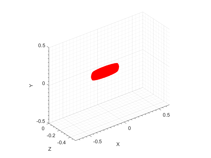
Model 1: An ellipsoid with principal semi-major axis and two semi-minor axes, respectively, being 0.2 (6 cm), 0.12 (3.6 cm) and 0.04 (1.2 cm) in and directions respectively. This ellipsoid has the dielectric constant .
-
•
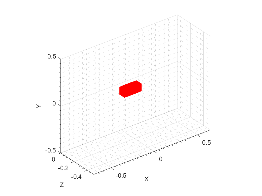
Model 2: A rectangular prism with dimensions (LWH) corresponding to in . It has the dielectric constant .
Remark 5.2.
These two examples model well the so-called “appearing” dielectric constant of metallic objects we experimented with in [41]. It was established numerically in [41] that the range of the appearing dielectric constant of metals is . Moreover, this range includes the dielectric constant 23.8 of the experimental watered glass bottle in [19]. Both metallic and glass bodied land mines are frequently used in the battlefields.
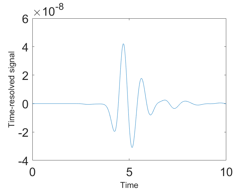
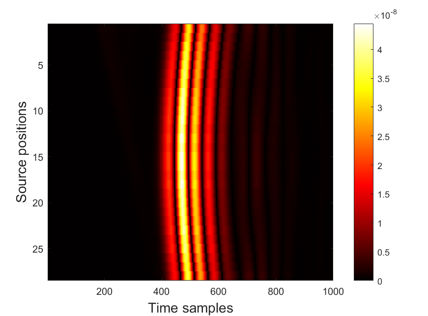
Suppose that our SAR data are for each and . Recall that is the source location number on the line of sources number . Prior of getting the data and in (3.6), we perform a data preprocessing procedure to filter out unwanted artifacts observed in the time-resolved signals. First, we eliminate small “peaks” of the signals by setting:
| (5.1) |
Second, we use the built-in function findpeaks in MATLAB to count the number of the peaks. Then, we deliberately keep only two first peaks of the signals because we believe that those are the most important ones for the object. The resulting signals are denoted by . We continue our preprocessing procedure by applying the delay-and-sum technique to as in [10]. For brevity, we do not detail internal steps of this data preprocessing procedure, but refer to [10, section III-A].
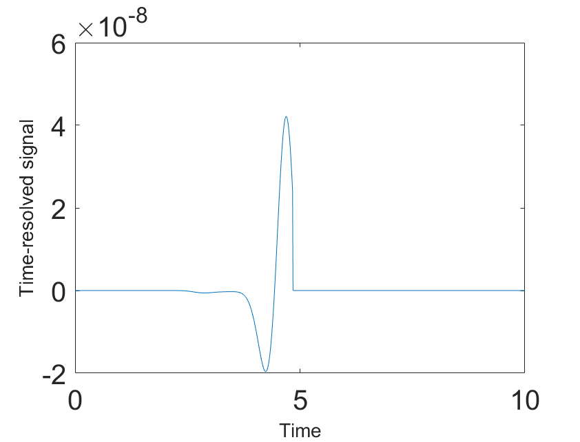
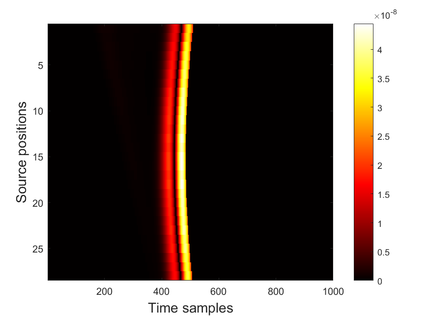
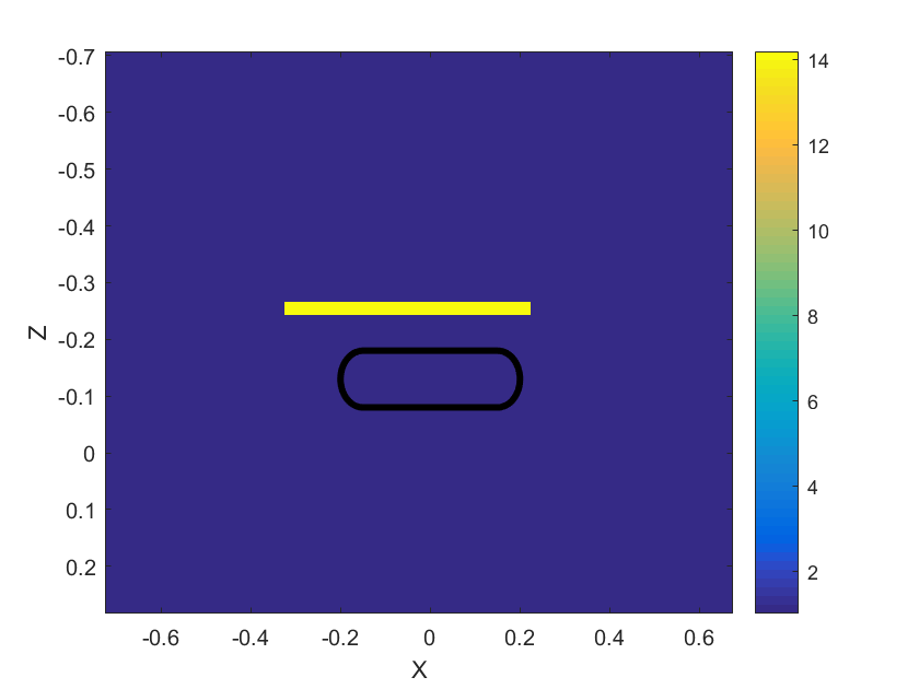
Now we focus on the preprocessing on the delay-and-sum data. In this context, for each line of source, the data are along the slant range planes which we reconstruct. Let be the slant range plane which corresponds to the line of sources In this plane , we, slightly abusing the same notations, consider as the source number and as the variable for the axis orthogonal to the line of source . Those are actually the transformation of using time of arrival. Thereby, we denote the delay-and-sum data by . We now introduce a truncation to control the size of the computed object. The “heuristically” truncated delay-and-sum data are given by
| (5.2) |
This way, we use only the absolute values as the data for each 1D inverse problem along the central line of the antenna. We also remark that the argument of [19, Remark 4] implies that the Neumann data equals to the derivative of , i.e. Our data preprocessing is exemplified in Figures 2a–2d.
To illustrate how our forward model works, consider Model 1 as an example. This object is centered at . The central point of the source line is located at . Therefore, the distance between these two points is . Hence, the backscattering time-resolved signal should bump at the point of the time domain. This is approximately the point we observe in Figure 2a. More precisely, our approximate signal bumps at the point , which is 10% difference with . But given that we have the whole ellipsoid rather than just its central point, this difference is acceptable for our simulations. This confirms how reliable our forward solver is. We can stop looking for the wave after the object’s bumps, which is after around the point ; see again Figure 2a. However, we enlarge the time domain up to the point to avoid any possible boundary reflections of the wave propagation. Moreover, we take into account 1000 time samples in Figure 2b to identify well the location of every wave with respect to .
For each line of sources, we use the truncation (5.2) to form a rectangular area . As mentioned above when considering variables , this rectangle is used in the slant range plane involving the transformation of in using times of arrival.
Remark 5.3.
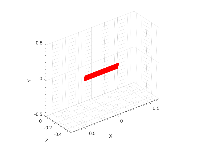
The selection of this rectangular region explains the reason why our computed objects in Figures 3b, 3c and Figures 4b, 4c have the rectangle-like shape. We are not focusing our work on the shape of the object since it is very challenging. Rather, we are interested in the accuracy of the computed dielectric constant of our two models. We are also interested in the dimensions of the computed object, and the presence of the above-mentioned rectangular region is helpful in controlling those dimensions.
Given a slant range plane we solve 1-D CIPs for sources Let the corresponding discrete solutions be discrete functions defined in . Note again that slightly abusing notation, the variable here is the grid point in . To reduce the artifacts, we average all the 1D solutions in our rectangular area . To do so, for each , we define first the semi-discrete function for as
| (5.3) |
since our domain of interest of the dielectric constant is [10,30]. Thus, for each source line of sources , our computed slant-range solution in , denoted by , is computed by
| (5.4) |
We define our computed slant-range solution in each slant range plane by (5.4) because from the above preprocessing data, we expect our inclusion in only the rectangle area. Therefore, it is relevant that the dielectric constant outside of that area should be unity. Finally, having all computed slant-range solutions , we assign one value of the final dielectric constant of our object by averaging the maximum values of those solutions. In particular, let and let be the prism formed by 3 slant-range planes . We then compute
| (5.5) |
In addition, we do the linear interpolation with respect to to help improve the resolution of images.
5.3. Computational results
We now first bring in our results for the case of noiseless data and then for the case of noisy data.
5.3.1. Noiseless data
In the case of Model 1, our computed dielectric constant for the ellipsoid , compared with the true value . For Model 2, the computed dielectric constant for the rectangular prism is , compared with the true value . Therefore, our approximations of the dielectric constants are quite accurate.
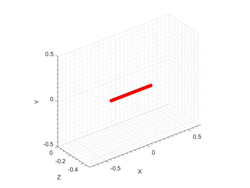
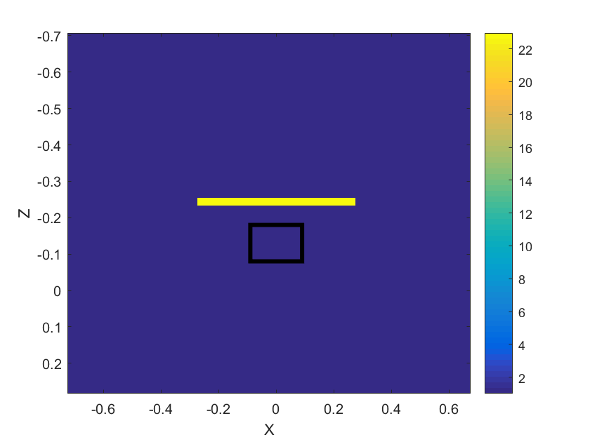
We now comment on dimensions of computed images. Recall that by Remark 5.3 our images have only rectangular shapes. One can see in Figures 3a and 3b that the dimensions of the computed ellipsoid of Model 1 are about (). On the other hand, dimensions of the true ellipsoid are (). This means that the computed object is longer in length, but smaller in width and is the same in height. Similarly, for Model 2, one can see in Figures 4a and 4b that the dimensions of the computed prism are (), while dimensions of the true prism are (). Hence, the computed prism is longer in length but smaller in width and height than the true prism.
5.3.2. Noisy data
While the above results are for the case of the noiseless data, we now introduce a noise in the data. We add a random additive noise to the truncated simulated data (see (5.1)). In this regard, we introduce
| (5.6) |
Here, represents the noise level and “rand” is a random number uniformly distributed in the interval . We use now the noisy data (5.6) for both Models 1 and 2 with which is of noise.
The resulting computed dielectric constant for the ellipsoid is , compared with the true value . For Model 2, our computed dielectric constant for the rectangular prism is , compared with the true value . In both models images for noisy data are about the same as the ones on Figures 3 and 4 for noiseless data.
6. Concluding remarks
In summary, we have numerically tested the convexification-based nonlinear SAR (CONSAR) imaging on identifying images of the dielectric constant of buried objects in a three-dimensional setting. We have numerically observed provides accurate values of dielectric constants of targets. However, the computed locations and sizes of tested targets are not as accurate as the convexification usually provides for conventional CIPs, see, e.g. the works of this research group for applications oof the convexification to experimental data [17, 18]. We hope to address these questions in follow up publications.
Acknowledgment
Vo Anh Khoa acknowledges Professor Taufiquar Khan (University of North Carolina at Charlotte) for the moral support of his research career.
References
- [1]
- [2] M. Amin, Through-the-wall Radar Imaging, CRC Press, Boca Raton, FL, 2011.
- [3] S. A. Carn, Application of synthetic aperture radar (SAR) imagery to volcano mapping in the humid tropics: a case study in East Java, Indonesia, Bulletin of Volcanology 61 (1-2) (1999) 92–105. doi:10.1007/s004450050265.
- [4] G. Chavent, Nonlinear Least Squares for Inverse Problems: Theoretical Foundations and Step-by-Step Guide for Applications, Scientic Computation, Springer, New York, 2009.
- [5] A. V. Goncharsky and S.Y. Romanov, Iterative methods for solving coefficient inverse problems of wave tomography in models with attenuation, Inverse Problems, 33, 025003, 2017.
- [6] A. V. Goncharsky and S.Y. Romanov, A method of solving the coefficient inverse problems of wave tomography Computers and Mathematics with Applications, 77, 967–980, 2019.
- [7] M. Gilman, E. Smith, S. Tsynkov, Transionospheric Synthetic Aperture Imaging, Springer International Publishing, 2017. doi:10.1007/978-3-319-52127-5.
- [8] S. Rotheram, J. T. Macklin, Inverse Methods for Ocean Wave Imaging by SAR, in: Inverse Methods in Electromagnetic Imaging, Springer Netherlands, 1985, pp. 907–930. doi:10.1007/978-94-009-5271-3_11.
- [9] L. Nguyen, M. Ressler, J. Sichina, Sensing through the wall imaging using the Army Research Lab ultra-wideband synchronous impulse reconstruction (UWB SIRE) radar, in: K. I. Ranney, A. W. Doerry (Eds.), Radar Sensor Technology XII, SPIE, 2008. doi:10.1117/12.776869.
- [10] M. V. Klibanov, A. V. Smirnov, V. A. Khoa, A. J. Sullivan, L. H. Nguyen, Through-the-wall nonlinear SAR imaging, IEEE Transactions on Geoscience and Remote Sensing 59 (9) (2021) 7475–7486. doi: 10.1109/TGRS.2021.3055805
- [11] M. V. Klibanov, N. T. Thành, Recovering dielectric constants of explosives via a globally strictly convex cost functional, SIAM Journal on Applied Mathematics 75 (2) (2015) 518–537. doi:10.1137/140981198.
- [12] N. T. Thành, L. Beilina, M. V. Klibanov, M. A. Fiddy, Imaging of buried objects from experimental backscattering time-dependent measurements using a globally convergent inverse algorithm, SIAM Journal on Imaging Sciences 8 (1) (2015) 757–786. doi:10.1137/140972469.
- [13] A. E. Kolesov, M. V. Klibanov, L. H. Nguyen, D.-L. Nguyen, N. T. Thành, Single measurement experimental data for an inverse medium problem inverted by a multi-frequency globally convergent numerical method, Applied Numerical Mathematics 120 (2017) 176–196. doi:10.1016/j.apnum.2017.05.007.
- [14] D.-L. Nguyen, M. V. Klibanov, L. H. Nguyen, M. A. Fiddy, Imaging of buried objects from multi-frequency experimental data using a globally convergent inversion method, Journal of Inverse and Ill-posed Problems 26 (4) (2018) 501–522. doi:10.1515/jiip-2017-0047.
- [15] M. V. Klibanov, A. E. Kolesov, D.-L. Nguyen, Convexification method for an inverse scattering problem and its performance for experimental backscatter data for buried targets, SIAM Journal on Imaging Sciences 12 (1) (2019) 576–603. doi:10.1137/18m1191658.
- [16] V. A. Khoa, M. V. Klibanov, L. H. Nguyen, Convexification for a three-dimensional inverse scattering problem with the moving point source, SIAM Journal on Imaging Sciences 13 (2) (2020) 871–904. doi:10.1137/19m1303101.
- [17] V. A. Khoa, G. W. Bidney, M. V. Klibanov, L. H. Nguyen, L. H. Nguyen, A. J. Sullivan, V. N. Astratov, Convexification and experimental data for a 3D inverse scattering problem with the moving point source, Inverse Problems 36 (8) (2020) 085007. doi:10.1088/1361-6420/ab95aa.
- [18] V. A. Khoa, G. W. Bidney, M. V. Klibanov, L. H. Nguyen, L. H. Nguyen, A. J. Sullivan, V. N. Astratov, An inverse problem of a simultaneous reconstruction of the dielectric constant and conductivity from experimental backscattering data, Inverse Problems in Science and Engineering (2020) 1–24. doi:10.1080/17415977.2020.1802447.
- [19] M. V. Klibanov, V. A. Khoa, A. V. Smirnov, L. H. Nguyen, G. W. Bidney, L. H. Nguyen, A. J. Sullivan, V. N. Astratov, Convexification inversion method for nonlinear SAR imaging with experimentally collected data, Journal of Applied and Industrial Mathematics 15 (3) (2021) 413–436. doi:10.1134/S1990478921030054.
- [20] A. V. Smirnov, M. V. Klibanov, A. J. Sullivan, L. H. Nguyen, Convexification for an inverse problem for a 1D wave equation with experimental data, Inverse Problems 36 (9) (2020) 095008. doi:10.1088/1361-6420/abac9a.
- [21] M. V. Klibanov, O. V. Ioussoupova, Uniform strict convexity of a cost functional for three-dimensional inverse scattering problem, SIAM Journal on Mathematical Analysis 26 (1) (1995) 147–179. doi:10.1137/s0036141093244039.
- [22] M. V. Klibanov, Global convexity in a three-dimensional inverse acoustic problem, SIAM Journal on Mathematical Analysis 28 (6) (1997) 1371–1388. doi:10.1137/s0036141096297364.
- [23] A. B. Bakushinskii, M. V. Klibanov, N. A. Koshev, Carleman weight functions for a globally convergent numerical method for ill-posed Cauchy problems for some quasilinear PDEs, Nonlinear Analysis: Real World Applications 34 (2017) 201–224. doi:10.1016/j.nonrwa.2016.08.008.
- [24] M. V. Klibanov, J. Li, Inverse Problems and Carleman Estimates, De Gruyter, 2021. doi:10.1515/9783110745481.
- [25] A. L. Bukhgeim, M. V. Klibanov, Uniqueness in the large of a class of multidimensional inverseproblems, Soviet Mathematics Doklady 17 (1981) 244–247.
- [26] L. Beilina, M. V. Klibanov, Approximate Global Convergence and Adaptivity for Coefficient Inverse Problems, Springer US, 2012. doi:10.1007/978-1-4419-7805-9.
- [27] M. Bellassoued, M. Yamamoto, Carleman Estimates and Applications to Inverse Problems for Hyperbolic Systems, Springer Japan, 2017. doi:10.1007/978-4-431-56600-7.
- [28] M. V. Klibanov, A. A. Timonov, Carleman Estimates for Coefficient Inverse Problems and Numerical Applications, VSP, Utrecht, 2004. doi:10.1515/9783110915549.
- [29] M. V. Klibanov, Carleman estimates for global uniqueness, stability and numerical methods for coefficient inverse problems, Journal of Inverse and Ill-Posed Problems 21 (4) (2013). doi:10.1515/jip-2012-0072.
- [30] M. Yamamoto, Carleman estimates for parabolic equations and applications, Inverse Problems 25 (12) (2009) 123013. doi:10.1088/0266-5611/25/12/123013.
- [31] N. V. Alekseenko, V. A. Burov, O. D. Rumyantseva, Solution of the three-dimensional acoustic inverse scattering problem. The modified Novikov algorithm, Acoustical Physics 54 (3) (2008) 407–419. doi:10.1134/s1063771008030172.
- [32] R. Novikov, The -approach to approximate inverse scattering at fixed energy in three dimensions, International Mathematics Research Papers 2005 (6) (2005) 287–349. doi:10.1155/imrp.2005.287.
- [33] G. A. Showman, Stripmap SAR, in: Principles of Modern Radar: Advanced techniques, Institution of Engineering and Technology, pp. 259–335. doi:10.1049/sbra020e_ch7.
- [34] R. A. Renaut, Absorbing boundary conditions, difference operators, and stability, Journal of Computational Physics 100 (2) (1992) 434. doi:10.1016/0021-9991(92)90257-y.
- [35] V. G. Romanov, Inverse Problems of Mathematical Physics, Walter de Gruyter GmbH & Co.KG, 2019.
- [36] A. Smirnov, M. Klibanov, L. Nguyen, Convexification for a 1D hyperbolic coefficient inverse problem with single measurement data, Inverse Problems & Imaging 14 (5) (2020) 913–938. doi:10.3934/ipi.2020042.
- [37] A. N. Tikhonov, Numerical Methods for the Solution of Ill-Posed Problems, Springer Netherlands, Dordrecht, 1995.
- [38] M. V. Klibanov, A. E. Kolesov, A. Sullivan, L. Nguyen, A new version of the convexification method for a 1D coefficient inverse problem with experimental data, Inverse Problems 34 (11) (2018) 115014. doi:10.1088/1361-6420/aadbc6.
- [39] M. V. Klibanov, A. E. Kolesov, Convexification of a 3-D coefficient inverse scattering problem, Computers & Mathematics with Applications 77 (6) (2019) 1681–1702. doi:10.1016/j.camwa.2018.03.016.
- [40] D. J. Daniels, A review of GPR for landmine detection, Sensing and Imaging: An International Journal 7 (3) (2006) 90–123. doi:10.1007/s11220-006-0024-5.
- [41] A. V. Kuzhuget, L. Beilina, M. V. Klibanov, A. Sullivan, L. Nguyen, M. A. Fiddy, Blind backscattering experimental data collected in the field and an approximately globally convergent inverse algorithm, Inverse Problems 28 (9) (2012) 095007. doi:10.1088/0266-5611/28/9/095007.
- [42] A. Lipson, S. G. Lipson, H. Lipson, Optical Physics, Cambridge University Press, 2018.