Numerical computation of second order vacuum perturbations of Kerr black holes

Justin L. Ripley [email protected] DAMTP, Centre for Mathematical Sciences, University of Cambridge, Wilberforce Road, Cambridge CB3 0WA, UK. Nicholas Loutrel [email protected] Department of Physics, Princeton University, Princeton, New Jersey 08544, USA. Elena Giorgi [email protected] Department of Mathematics, Princeton University, Princeton, New Jersey 08544, USA. Princeton Gravity Initiative, Princeton University, Princeton, New Jersey 08544, USA. Frans Pretorius [email protected] Department of Physics, Princeton University, Princeton, New Jersey 08544, USA. Princeton Gravity Initiative, Princeton University, Princeton, New Jersey 08544, USA.

Abstract

Motivated by the desire to understand the leading order nonlinear gravitational wave interactions around arbitrarily rapidly rotating Kerr black holes, we describe a numerical code designed to compute second order vacuum perturbations on such spacetimes. A general discussion of the formalism we use is presented in Loutrel et al. (2020); here we show how we numerically implement that formalism with a particular choice of coordinates and tetrad conditions, and give example results for black holes with dimensionless spin parameters $a=0.7$ and $a=0.998$ . We first solve the Teukolsky equation for the linearly perturbed Weyl scalar $\Psi_{4}^{(1)}$ , followed by direct reconstruction of the spacetime metric from $\Psi_{4}^{(1)}$ , and then solve for the dynamics of the second order perturbed Weyl scalar $\Psi_{4}^{(2)}$ . This code is a first step toward a more general purpose second order code, and we outline how our basic approach could be further developed to address current questions of interest, including extending the analysis of ringdown in black hole mergers to before the linear regime, exploring gravitational wave “turbulence” around near-extremal Kerr black holes, and studying the physics of extreme mass ratio inspiral.

I Introduction

In this paper we initiate a numerical study of the dynamics of second order vacuum perturbations of a Kerr black hole. Linear black hole perturbation theory has played an important role in the study of black holes, with diverse applications from mathematical physics to gravitational wave astrophysics (for reviews see e.g. Sasaki and Tagoshi (2003); Dafermos and Rodnianski (2013); Barack and Pound (2019)). Regarding the latter, it is used in interpreting the ringdown phase of a binary black hole merger, and for extreme mass ratio inspirals (EMRIs). For both of these physical regimes, it is presently computationally intractable to full numerical solution without recourse to perturbative methods.

For some applications it may be necessary to go beyond linear perturbations. Here for brevity we only mention a couple of key incentives (a more thorough discussion that motivates this study can be found in our companion paper Loutrel et al. (2020)). In order to extract subleading modes of the ringdown following comparable mass mergers, it may be necessary to consider nonlinear effects. The “problem” with such mergers is that the leading order quadrupole mode is excited with such high amplitude relative to subleading modes (see e.g. London et al. (2014, 2016)), that nonlinear mode coupling could produce features of similar strength to subleading modes; this is particularly so within the first few cycles of ringdown were most of the observable signal, hence most opportunity for measurement, lies. It will be important to quantitatively understand second order features to reap the most out of ringdown analysis of future loud merger events.

Nonlinear physics may also play an important role in the ringdown of near-extremal Kerr black holes¹¹1We note though that comparable mass mergers cannot produce near-extremal remnants, see e.g. Hemberger et al. (2013); Lousto and Zlochower (2014); Healy et al. (2014); Hofmann et al. (2016), and it is unknown how rapidly the typical supermassive black holes in the universe, of relevance to EMRIs, rotate. Thus near-extremal ringdown may end up being more a question of theoretical, rather than astrophysical, interest. . This can partly be motivated by the presence of a family of slowly damped modes, whose damping timescale grows without bound as the black hole spin approaches its extremal value Detweiler (1980); Hod (2008); Yang et al. (2013)²²2Though there is some controversy about exactly what the spectrum of modes of extremal/near-extremal black holes is; see e.g. Hod (2015); Zimmerman et al. (2015); Hod (2016); Richartz (2016); Casals and Longo Micchi (2019).. The slower damping of perturbations implies nonlinear effects could be more pronounced; most intriguing in this regard is the suggestion that mode coupling induces a turbulent energy cascade in near-extremal Kerr black holes Yang et al. (2015), similar to that seen in a few studies of black holes and black branes in asymptotically Anti de-Sitter spacetime Carrasco et al. (2012); Green et al. (2014); Adams et al. (2014). Nonlinear effects almost certainly play some role in the physics of extremal Kerr black holes, as those have been shown to be linearly unstable Detweiler (1980); Aretakis (2015, 2013) (the instability may be related to the above mentioned slowly damped quasinormal modes, that become “zero damped” in the extremal limit).

Finally, we mention that second order black hole perturbation theory plays an important role in computing the second order self force of a small particle orbiting a black hole, which is relevant to modeling EMRIs (e.g. Barack (2009)). We note though that in this paper we only consider the second order vacuum perturbation of a Kerr black hole, so our results are not directly applicable to modeling EMRI physics.

Following a brief summary of our formalism in Sec.II.1 (which is described in more detail in our companion paper Loutrel et al. (2020)), in the remainder of this paper we describe a numerical implementation of the method and then analyze a few example runs from our code. In the remainder of the introduction we give a general overview of our numerical approach.

Several steps are required to arrive at the desired second order perturbation. First is to solve for a linear gravitational wave perturbation characterized by the Weyl scalar $\Psi_{4}$ (or equivalently $\Psi_{0}$ ) using the Teukolsky equation Teukolsky (1973). As described in Sec. II.2, with more details given in Appendix C, we begin with the Kerr metric in Boyer-Lindquist form and a rotated version of the Kinnersley tetrad Kinnersley (1969), then transform these to a hyperboloidal compactified, horizon penetrating coordinate system. In these coordinates then we numerically solve the Teukolsky equation in the time domain, starting with Cauchy data for $\Psi_{4}^{(1)}$ . (We note that many codes have been developed over the years to solve the Teukolsky equation; see, e.g. Krivan et al. (1997, 1997); Baker et al. (2002); Lopez-Aleman et al. (2003); Lousto (2005); Burko and Khanna (2007); Sundararajan et al. (2007); Zenginoglu and Khanna (2011); Harms et al. (2013)).

Campanelli and Lousto first showed that the evolution of the second order perturbation of $\Psi_{4}$ is also governed by the Teukolsky equation, with a source term that depends on all components of the first order metric perturbation $h_{\mu\nu}$ Campanelli and Lousto (1999). The next step in our calculation the is therefore to reconstruct this first order metric correction from the first order perturbation of $\Psi_{4}$ . We directly reconstruct the metric by solving a set of nested null transport equations in the outgoing radiation gauge Chrzanowski (1975). Once this is complete, we numerically solve the Teukolsky equation in the time domain with the second order source term for the second order correction to $\Psi_{4}$ . This latter quantity is in general not invariant under first order gauge or tetrad transformations (see Campanelli and Lousto (1999)); as discussed in Sec. III, in our coordinate system we can avoid these issues if we measure the waves at future null infinity in an asymptotically flat gauge, which is one reason why we employ a hyperboloidal slicing and the outgoing radiation gauge.

Refer to caption — Figure 1: Schematic Penrose diagram demonstrating the domains of evolution and metric reconstruction. The Teukolsky equation is integrated using a Cauchy evolution scheme along hypersurfaces of constant time $T$ , whereas metric reconstruction is carried out using null transport equations in the $u$ direction, with characteristics tangent to the ingoing Newman-Penrose vector $n^{\mu}$ . We provide initial data for the first order $\Psi_{4}^{(1)}$ at $T=0$ , with compact support in radial distance from the black hole in the range $r=(r_{l},r_{u})$ , intersecting a range in advanced (retarded) time of $u=(u_{u},u_{l})$ ( $v=(v_{l},v_{u})$ ). Thus only in the region $u>u_{u},T>0,$ does the spacetime differ from Kerr, which allows for trivial initial data for the first order metric reconstruction equations along $u=u_{u}$ . For simplicity, as explained in the text, we begin evolution of the second order perturbation $\Psi_{4}^{(2)}$ at $T=T_{s}$ ; in a sense then this is our “true” initial data surface for the gravitational wave perturbation of Kerr calculated to second order. For technical reasons explained in Sec. IV, this initial data setup only leads to consistent metric reconstruction if $\Psi_{4}^{(1)}$ has azimuthal mode content $|m|\geq 2$ .

One difficulty with using null transport equations in conjunction with the (3+1) Cauchy evolution scheme we use for the Teukolsky equation is that their domains of integration do not “easily” overlap. An implication of this is if we wanted to solve for the second order perturbation over the entire domain of our Cauchy evolution we would need to solve a set of first order constraint equations on the initial $T=0$ slice to give self-consistent initial data for the reconstruction equations. As explained more in Sec. IV and illustrated in Fig. 1, we avoid this issue here by choosing initial data for the first-order $\Psi_{4}^{(1)}$ that has compact support on the initial slice, and only solve for the first order metric beginning on an ingoing null slice ( $v_{u}$ ) intersecting $T=0$ outside of this region (as we explain in Fig. 1, our metric reconstruction equations are transport equations along the ingoing null tetrad vector $n^{\mu}$ ). Then, initial data for reconstruction only needs to be specified along the outgoing null curves $u=u_{u}$ , which is trivially the Kerr solution. In principle we could immediately begin the second order evolution for $v\geq v_{u}$ , though again to simplify the Cauchy evolution we only start second order evolution at a constant hyperboloidal time $T_{s}$ after all the ingoing data from $v_{l}$ to $v_{u}$ has entered the black hole horizon. The Cauchy evolution prior to this is then, in a sense, simply providing a map from initial data for the first order $\Psi_{4}^{(1)}$ specified on $T=0$ to the “true” initial time $T=T_{s}$ . As implemented in the code, during each step of the Cauchy evolution we also perform reconstruction (and second order integration for $T>T_{s}$ ). The reconstruction will therefore not be consistent until evolution crosses $v=v_{u}$ , but for illustrative purposes we also show independent residuals of our reconstruction procedure prior to that, to demonstrate that the inconsistency then has no effect on the consistency of the solution afterward.

As described in Sec.V, we use pseudo-spectral methods to solve both the Teukolsky and null transport equations; the code can be downloaded from Ripley (2020a). Example results are given in Sec. VI.1 and Sec. VI.2 for a black hole with dimensionless spin $a=0.7$ and $a=0.998$ respectively. Specifically, for the examples we consider the linear wave only contains azimuthal $e^{im\phi}$ angular dependence for $m=2$ . This linear field sources a second order $\Psi_{4}^{(2)}$ containing modes with both $m=0$ and $m=4$ . We conclude in Sec. VII, which includes a discussion of how our methods and code will be extended to tackle the problems we are ultimately interested in addressing.

In Appendix A we describe the conventions we use for the Fourier transform and normalization of discrete quantities used to display some of our results. In Appendix B we provide a derivation of the metric reconstruction equations and second order source term in the specific gauge and coordinates used here, which is slightly different from the analytical example case give in Loutrel et al. (2020). We describe the transformation of the Kerr metric and Kinnersley tetrad in Boyer-Lindquist coordinates to the coordinates we use in the code in Appendix C. Finally, in Appendix D we collect some useful properties of spin-weighted spherical harmonics, which are used in our pseudo-spectral code.

I.1 Notation and conventions

We use geometric units ( $8\pi G=1$ , $c=1$ ) and follow the definitions and sign conventions of Chandrasekhar Chandrasekhar (2002) (in particular the $+---$ signature for the metric), except we use Greek letters $\mu,\nu...$ to denote spacetime indices. We use the non-standard symbols : $\varpi=3.14159...$ for the number ‘pi’ (to avoid confusion with the Newman-Penrose scalar $\pi$ ), and the symbols $\mathcal{R}$ and $\mathcal{I}$ to respectively denote the real and imaginary parts of fields. We use an overbar $\bar{f}$ to denote complex conjugation of a quantity $f$ .

We write the perturbed metric $g_{\mu\nu}$ about a background solution $g_{\mu\nu}^{(0)}$ as $g_{\mu\nu}=g_{\mu\nu}^{(0)}+h_{\mu\nu}$ , where $h_{\mu\nu}$ is the first order perturbation. Other than the metric, we denote an $n^{th}$ order quantity in a perturbative expansion with a trailing superscript $\ {}^{(n)}$ ; e.g. the Newman-Penrose scalar $\Psi_{2}=\Psi_{2}^{(0)}+\Psi_{2}^{(1)}$ to linear order. However, for brevity, in terms of expressions where the correction to a background quantity will lead to a higher order perturbation than considered, we drop the ⁽⁰⁾ superscript from the background quantity. For example, in the Teukolsky equation, Eq. (II.1) below, all symbols other than $\Psi_{4}^{(1)}$ are background quantities.

II Description of the Scheme

In this section we summarize details of the reconstruction scheme and second order perturbation equation described in Loutrel et al. (2020) that are particular to our numerical implementation.

II.1 Use of the NP/GHP formalisms

We make extensive use of the Newman-Penrose (NP)Newman and Penrose (1962) formalism. In the Appendix of the companion paper Loutrel et al. (2020) we gave a brief overview of the NP formalism, and to avoid excessive repetition we do not reproduce that here. However, we now mention the most salient definitions of the NP formalism necessary to understand the main points of this paper.

The NP formalism decomposes the geometry and Einstein equations in terms of an orthonormal basis of null vectors, $\{l^{\mu},n^{\mu},m^{\mu},\bar{m}^{\mu}\}$ ; $l^{\mu}$ ( $n^{\mu}$ ) is an outgoing (ingoing) real null vector, and $m^{\mu}$ is a complex angular null vector with $\bar{m}^{\mu}$ its complex conjugate. These define the four directional derivative operators

	$\displaystyle{D}$	$\displaystyle=$	$\displaystyle l^{\mu}\partial_{\mu}\,,\qquad{\Delta}=n^{\mu}\partial_{\mu}\,,$		(1)
	$\displaystyle{\delta}$	$\displaystyle=$	$\displaystyle m^{\mu}\partial_{\mu}\,,\qquad\bar{{\delta}}=\bar{m}^{\mu}\partial_{\mu}\,.$		(2)

A vacuum geometry is characterized by the 5 complex scalars $\{\Psi_{0},\Psi_{1},\Psi_{2},\Psi_{3},\Psi_{4}\}$ , which are contractions of the Weyl tensor with various products of the null tetrad. The complex spin coefficients (essentially combinations of Ricci rotation coefficients, the tetrad analogue of the connection in a metric formalism) are $\{\alpha,\beta,\gamma,\epsilon,\rho,\lambda,\pi,\mu,\nu,\tau,\sigma,\kappa\}$ . We choose a null tetrad, the explicit form of which is given later, such that for the background Kerr solution $\Psi_{0}=\Psi_{1}=\Psi_{3}=\Psi_{4}=\sigma=\kappa=\nu=\lambda=0$ (which is always possible for a general type D background) and $\gamma=0$ (which is always possible when the background is Kerr).

In the NP formalism, perturbations of the Kerr spacetime lead to one master equation for the linearly perturbed Weyl scalar $\Psi_{4}$ known as the Teukolsky equation Teukolsky (1973), specifically

	$\displaystyle\mathcal{T}\Psi_{4}^{(1)}\equiv\big{[}\left(\Delta+4\mu+\bar{\mu}\right)\left(D+4\epsilon-\rho\right)$
	$\displaystyle-\left(\textnormal{\dh}^{\prime}+4\pi-\bar{\tau}\right)\left(\textnormal{\dh}-\tau\right)-3\Psi_{2}\big{]}\Psi_{4}^{(1)}=0.$		(3)

(Here we have made use of the GHP operators ð and $\textnormal{\dh}^{\prime}$ , which we define in Eq. (4).) The first step of our procedure is to solve the Teukolsky equation for $\Psi_{4}^{(1)}$ . We discuss how we numerically solve this equation in Sec. V.1.

We also make some use of the Geroch-Held-Penrose (GHP) Geroch et al. (1973) formalism; in particular we use the following GHP derivatives acting on some NP scalar $\eta$


	$\displaystyle\textnormal{\dh}\eta\equiv\left(\delta-p\beta-q\bar{\alpha}\right)\eta,$		(4a)
	$\displaystyle\textnormal{\dh}^{\prime}\eta\equiv\left(\bar{\delta}-p\alpha-q\bar{\beta}\right)\eta,$		(4b)

where $\{p,q\}$ are the (constant) weights of $\eta$ (related to its spin and boost weights).

II.2 Choice of background coordinates and tetrad

We choose a form for the background Kerr metric, with mass and spin parameters $M$ and $a$ respectively, that is horizon penetrating and hyperboloidally compactified so that the constant time $T$ (spacelike) slices become asymptotically null, reaching future null infinite at finite coordinate radius. An outline of how we derive these coordinates is given in Appendix C; here we simply summarize their most important qualities.

We use a rotated version of the Kinnersley tetrad that is regular at future null infinity; in $(T,R,\vartheta,\phi)$ component form, the tetrad vectors read:


$\displaystyle l^{\mu}=$	$\displaystyle\frac{R^{2}}{L^{4}+a^{2}R^{2}\mathrm{cos}^{2}\vartheta}\bigg{(}2M\left(2M-\left(\frac{a}{L}\right)^{2}R\right),$
	$\displaystyle-\frac{1}{2}\left(L^{2}-2MR+\left(\frac{a}{L}\right)^{2}R^{2}\right),0,a\bigg{)},$	(5a)
$\displaystyle n^{\mu}=$	$\displaystyle\left(2+\frac{4MR}{L^{2}},\frac{R^{2}}{L^{2}},0,0\right),$	(5b)
$\displaystyle m^{\mu}=$	$\displaystyle\frac{R}{\sqrt{2}\left(L^{2}-iaR\mathrm{cos}\vartheta\right)}\left(-ia\mathrm{sin}\vartheta,0,-1,-\frac{i}{\mathrm{sin}\vartheta}\right).$	(5c)

Here $R$ is the compactified radial coordinate, related to the Boyer-Lindquist radial coordinate by

\displaystyle r\equiv\frac{L^{2}}{R},

(6)

with $L$ a constant parameter ( $R=0$ thus corresponds to future null infinity).

With this tetrad and metric, the only nonzero Weyl scalar is

\displaystyle\Psi_{2}=-\frac{MR^{3}}{\left(L^{2}-iaR\mathrm{cos}\left(\vartheta\right)\right)^{3}},

(7)

and the nonzero spin coefficients are


$\displaystyle\rho=$	$\displaystyle-\frac{R\left(a^{2}R^{2}+L^{4}-2L^{2}MR\right)}{2\left(L^{2}-iaR\cos(\vartheta)\right)^{2}\left(L^{2}+iaR\cos(\vartheta)\right)},$	(8a)
$\displaystyle\mu=$	$\displaystyle\frac{R}{-L^{2}+iaR\cos(\vartheta)},$	(8b)
$\displaystyle\tau=$	$\displaystyle\frac{iaR^{2}\sin(\vartheta)}{\sqrt{2}\left(L^{2}-iaR\cos(\vartheta)\right)^{2}},$	(8c)
$\displaystyle\pi=$	$\displaystyle-\frac{iaR^{2}\sin(\vartheta)}{\sqrt{2}\left(a^{2}R^{2}\cos^{2}(\vartheta)+L^{4}\right)},$	(8d)
$\displaystyle\epsilon=$	$\displaystyle\frac{R^{2}\left(a^{2}(-R)-ia\cos(\vartheta)\left(L^{2}-MR\right)+L^{2}M\right)}{2\left(L^{2}-iaR\cos(\vartheta)\right)^{2}\left(L^{2}+iaR\cos(\vartheta)\right)},$	(8e)
$\displaystyle\alpha=$	$\displaystyle\frac{R\cot(\vartheta)}{\sqrt{2}\left(2L^{2}+2iaR\cos(\vartheta)\right)},$	(8f)
$\displaystyle\beta=$	$\displaystyle\frac{R\left(-L^{2}\cot(\vartheta)+iaR\sin(\vartheta)\left(\csc^{2}(\vartheta)+1\right)\right)}{2\sqrt{2}\left(L^{2}-iaR\cos(\vartheta)\right)^{2}}.$	(8g)

The coefficients $\alpha$ and $\beta$ are singular at the poles ( $\vartheta=0,\varpi$ ), but when expanded out in the equations of motion they only appear with other terms that in combination are regular there. Other than this, all spin coefficients are regular in the domain of interest, namely on the black hole horizon and the region exterior to it. Notice that with the Kinnersley tetrad $\epsilon=0$ , but we have rotated to a tetrad where $\gamma=0$ instead.

The quantities above are sufficient to completely determine the Teukolsky and metric reconstruction equations, and so for brevity we do not write out the explicit form of the Kerr metric in these coordinates.

II.3 Choice of linearized metric gauge and linearized tetrad

After computing $\Psi_{4}^{(1)}$ , we need to specify a gauge in which to reconstruct the first order metric; we choose the outgoing radiation gauge, defined by the following conditions:


$\displaystyle h_{\mu\nu}n^{\mu}=$	$\displaystyle 0,$	(9a)
$\displaystyle g^{\mu\nu}h_{\mu\nu}=$	$\displaystyle 0.$	(9b)

For type D background spacetimes one can always impose the outgoing (or ingoing) radiation gauge, despite the fact that this imposes five conditions on the linear metric Price et al. (2007). The only nonzero tetrad projections of $h_{\mu\nu}$ in outgoing radiation gauge are


$\displaystyle h_{ll}\equiv$	$\displaystyle h_{\mu\nu}l^{\mu}l^{\nu},$	(10a)
$\displaystyle h_{lm}\equiv$	$\displaystyle h_{\mu\nu}l^{\mu}m^{\nu},$	(10b)
$\displaystyle h_{mm}\equiv$	$\displaystyle h_{\mu\nu}m^{\mu}m^{\nu},$	(10c)

and the complex conjugates of the last two, i.e. $h_{l\bar{m}}\equiv h_{\mu\nu}l^{\mu}\bar{m}^{\nu}$ and $h_{\bar{m}\bar{m}}\equiv h_{\mu\nu}\bar{m}^{\mu}\bar{m}^{\nu}$ .

As detailed in Appendix B, in this gauge we can choose the linearly perturbed tetrad vectors so that the first order corrections to the derivative operators are


$\displaystyle D^{(1)}=$	$\displaystyle-\frac{1}{2}h_{ll}\Delta,$	(11a)
$\displaystyle\Delta^{(1)}=$	$\displaystyle 0,$	(11b)
$\displaystyle\delta^{(1)}=$	$\displaystyle-h_{lm}\Delta+\frac{1}{2}h_{mm}\bar{\delta}.$	(11c)

II.4 Metric reconstruction equations

Our metric reconstruction procedure consists of solving a nested set of transport equations that are derived by linearly expanding some of the Bianchi and Ricci identities in the NP formalism; see Appendix B. Unlike metric reconstruction procedures that use “Hertz potentials” (see e.g. Chrzanowski (1975)), our method directly reconstructs the metric from $\Psi_{4}^{(1)}$ . The basic idea of this metric reconstruction procedure was first described by Chandrasekhar Chandrasekhar (2002). One advantage of our implementation of Chandrasekhar’s idea is that it does not require using any specific features of a particular coordinate system beyond the gauge and tetrad choices we have already stated; a similar approach has recently been rigorously analyzed by Andersson et. al. Andersson et al. (2019). A disadvantage of our implementation though is that outgoing radiation gauge is incompatible with most forms of source term, including from matter with a stress energy tensor that is not trace-free, or that coming from first order vacuum perturbations³³3We note though that the general approach of reconstructing the metric by solving a series of nested transport equations does not require one use the radiation gauges; indeed Chandrasekhar Chandrasekhar (2002) does not use a radiation gauge. For a brief review of recent works that directly reconstruct the metric: Andersson et. al. Andersson et al. (2019) works in outgoing radiation gauge for perturbations of Kerr, Dafermos et. al. Dafermos et al. (2019) work in a double null gauge for perturbations of Schwarzschild, and Klainerman and Szeftel Klainerman and Szeftel (2017) work in a Bondi gauge for perturbations of Schwarzschild. In a different gauge one could presumably reconstruct the metric in the presence of linearized matter perturbations. That being said, using a radiation gauge greatly simplifies and reduces the number of metric reconstruction equations that we need to solve, and is sufficient for solving for the dynamics of the second order Weyl scalar $\Psi_{4}^{(2)}$ about a Kerr background.. Therefore, we can compute the gravitational wave perturbation $\Psi_{4}$ to second order, but the metric tensor only to first order. Recently Green et al. (2020) proposed a method based (in part) on Hertz potentials that does not seem to have such restrictions. However, for our purposes we believe our method is more straightforward to implement (see our companion paper Loutrel et al. (2020) for more discussion on these different approaches to reconstruction).

Given a solution $\Psi_{4}^{(1)}$ to the Teukolsky equation, below are the transport equations we solve to reconstruct the first order metric:


$\displaystyle-\left(\Delta+4\mu\right)\Psi_{3}^{(1)}+\left(\textnormal{\dh}-\tau\right)\Psi_{4}^{(1)}$	$\displaystyle=0,$	(12a)
$\displaystyle-\left(\Delta+\mu+\bar{\mu}\right)\lambda^{(1)}-\Psi_{4}^{(1)}$	$\displaystyle=0,$	(12b)
$\displaystyle-\left(\Delta+3\mu\right)\Psi_{2}^{(1)}+\left(\textnormal{\dh}-2\tau\right)\Psi_{3}^{(1)}$	$\displaystyle=0,$	(12c)
$\displaystyle-\left(\Delta-\mu+\bar{\mu}\right)h_{\bar{m}\bar{m}}-2\lambda^{(1)}$	$\displaystyle=0,$	(12d)
$\displaystyle-\Delta\pi^{(1)}-\Psi_{3}^{(1)}-\left(\bar{\pi}+\tau\right)\lambda^{(1)}$
$\displaystyle+\frac{1}{2}\mu\left(\bar{\pi}+\tau\right)h_{\bar{m}\bar{m}}$	$\displaystyle=0,$	(12e)
$\displaystyle-\left(\Delta+\bar{\mu}\right)h_{l\bar{m}}-2\pi^{(1)}-\tau h_{\bar{m}\bar{m}}$	$\displaystyle=0,$	(12f)
$\displaystyle-\left(\Delta+\bar{\mu}\right)\left(\mu h_{ll}\right)-\mu\left(\textnormal{\dh}+\bar{\pi}+2\tau\right)h_{l\bar{m}}$
$\displaystyle-2\Psi_{2}^{(1)}-\pi\left(\textnormal{\dh}^{\prime}-\pi\right)h_{mm}$
$\displaystyle+\left(\mu\textnormal{\dh}^{\prime}-3\mu\pi+2\bar{\mu}\pi-2\mu\bar{\tau}\right)h_{lm}$
$\displaystyle-2\left(\textnormal{\dh}+\bar{\pi}\right)\pi^{(1)}-2\pi\bar{\pi}^{(1)}$	$\displaystyle=0.$	(12g)

We solve the equations in the sequence listed, in each step obtaining one of the following set of unknowns: $\{\Psi_{3}^{(1)},\lambda^{(1)},\Psi_{2}^{(1)},h_{\bar{m}\bar{m}},\pi^{(1)},h_{l\bar{m}},h_{ll}\}$ . We set the initial values for all these quantities to zero; as explained in the Introduction and Sec. IV, this choice is consistent from the ingoing slice $v=v_{u}$ shown in Fig.1 onward (i.e. for $v\geq v_{u}$ ), as long as the initial data for $\Psi_{4}^{(1)}$ only contains azimuthal modes $|m|\geq 2$ .

II.5 Source term for the second order perturbation $\Psi_{4}^{(2)}$

Having computed the linearized metric, we can then solve for the second order perturbation of the Weyl scalar, $\Psi_{4}^{(2)}$ . As was first shown in Campanelli and Lousto (1999), the equation of motion for $\Psi_{2}^{(2)}$ can be written as

\displaystyle\mathcal{T}\Psi_{4}^{(2)}=\mathcal{S}\left[h_{\mu\nu}\right],

(13)

where $\mathcal{T}$ is the Teukolsky operator (Eq. (II.1)), and $\mathcal{S}$ is the “source” term which depends on the first order perturbed metric. The general expression for $\mathcal{S}$ is given in Campanelli and Lousto (1999); Loutrel et al. (2020). Here we write it down in outgoing radiation gauge and with our background tetrad choice (see Appendix B for a derivation):

\displaystyle\mathcal{S}=\left(\Delta+4\mu+\bar{\mu}\right)\mathfrak{s}_{d}+\left(\textnormal{\dh}^{\prime}+4\pi-\bar{\tau}\right)\mathfrak{s}_{t},

(14)

where


$\displaystyle\mathfrak{s}_{d}\equiv$	$\displaystyle\frac{1}{2}h_{ll}\left(\Delta+\mu\right)\Psi_{4}^{(1)}+\Psi_{4}^{(1)}\bigg{[}\frac{1}{2}\left(\textnormal{\dh}+\bar{\pi}+2\tau\right)h_{l\bar{m}}$
	$\displaystyle+\left(\Delta-\mu+\bar{\mu}\right)h_{ll}-\frac{1}{2}\left(\textnormal{\dh}^{\prime}-5\pi-4\bar{\tau}\right)h_{lm}\bigg{]}$
	$\displaystyle-\frac{1}{2}\Psi_{3}^{(1)}\bigg{[}\left(\textnormal{\dh}+\bar{\pi}+\tau\right)h_{\bar{m}\bar{m}}+\left(\Delta-2\mu+\bar{\mu}\right)h_{l\bar{m}}\bigg{]}$
	$\displaystyle-\left(h_{l\bar{m}}\Delta-\frac{1}{2}h_{\bar{m}\bar{m}}\textnormal{\dh}-4\pi^{(1)}\right)\Psi_{3}^{(1)}-3\lambda^{(1)}\Psi_{2}^{(1)},$	(15a)
$\displaystyle\mathfrak{s}_{t}\equiv$	$\displaystyle-h_{lm}\left(\Delta+\mu+2\bar{\mu}\right)\Psi_{4}^{(1)}+\frac{1}{2}h_{mm}\textnormal{\dh}^{\prime}\Psi_{4}^{(1)}$
	$\displaystyle+\Psi_{4}^{(1)}\bigg{[}\bar{\pi}^{(1)}-\Delta h_{lm}+\left(\textnormal{\dh}^{\prime}-\frac{1}{2}\pi-\frac{1}{2}\bar{\tau}\right)h_{mm}\bigg{]}.$	(15b)

III Measurement of the gravitational wave at future null infinity

For outgoing radiation at future null infinity in an asymptotically flat coordinate system there is a simple relation between $\Psi_{4}^{(1)}$ and the linearized metric (e.g. Teukolsky (1973)):

\displaystyle\lim_{r\to\infty}\Psi_{4}^{(1)}=-\frac{1}{2}\left(\partial_{t}^{2}h_{+}-i\partial_{t}^{2}h_{\times}\right),

(16)

where the $+$ and $\times$ subscripts refer to the “plus” and “cross” polarizations of the gravitational wave. From this we can then also calculate other quantities of interest, such as the energy and angular momentum radiated to future null infinity.

As is discussed in Campanelli and Lousto (1999) (see Sec III.C and Sec. IV therein), $\Psi_{4}^{(2)}$ is in general not invariant under gauge or tetrad transformations that are first order in magnitude (it is invariant under second order transformations). This complicates the interpretation of $\Psi_{4}^{(2)}$ , unless the gauge/tetrad is fixed in an appropriate way, or as outlined in Campanelli and Lousto (1999), a gauge invariant object is calculated that by construction reduces to $\Psi_{4}^{(2)}$ in the desired gauge at null infinity. Here, because we use the outgoing radiation gauge in an asymptotically flat representation of Kerr, and our first order correction to the tetrad (50a) amounts to a Class II transformation that leaves $\Psi_{4}$ invariant Chandrasekhar (2002), we can directly interpret $\Psi_{4}^{(2)}$ as we do $\Psi_{4}^{(1)}$ in (16) at future null infinity; i.e. we can interpret the real and imaginary parts of $\Psi_{4}^{(2)}$ as the second time derivative of the plus and cross gravitational wave polarizations, respectively.

Another way to understand the physical interpretation of the second order gravational wave perturbation at future null infinity is through the radiated energy and angular momentum Campanelli and Lousto (1999):


$\displaystyle\frac{dE}{du}\Big{\|}_{\mathcal{J}_{+}}=$	$\displaystyle\lim_{r\to\infty}\left\{\frac{r^{2}}{4\pi}\int_{\Omega}d\Omega\left\|\int_{-\infty}^{u}du^{\prime}\Psi_{4}\right\|^{2}\right\}$	(17a)
$\displaystyle\frac{dJ_{z}}{du}\Big{\|}_{\mathcal{J}_{+}}=$	$\displaystyle-\lim_{r\to\infty}\mathcal{R}\Bigg{\{}\frac{r^{2}}{4\pi}\int_{\Omega}d\Omega\left(\partial_{\phi}\int_{-\infty}^{u}du^{\prime}\Psi_{4}\right)$
	$\displaystyle\times\left(\int_{-\infty}^{u}du^{\prime}\int_{-\infty}^{u^{\prime}}du^{\prime\prime}\Psi_{4}\right)\Bigg{\}}.$	(17b)

In computing $\Psi_{4}^{(2)}$ at future null infinity using outgoing radiation gauge to linear order, one can compute the linear and leading order nonlinear contribution to the radiated energy and angular momentum through future null infinity.

IV Initial data

As discussed in the introduction and illustrated in Fig. 1 there, on our $T=0$ initial data surface $\mathfrak{i}_{0}$ we set $\Psi_{4}^{(1)}$ to be nonzero and smooth over a compact region $\mathfrak{p}_{0}\subset\mathfrak{i}_{0}$ , and set the rest of our evolution variables (the metric reconstructed variables $\{h_{ll},h_{l\bar{m}},h_{\bar{m}\bar{m}},\Psi_{3}^{(1)},\Psi_{2}^{(1)},\lambda^{(1)},\pi^{(1)}\}$ , and $\Psi_{4}^{(2)}$ ) to be zero everywhere on $\mathfrak{i}_{0}$ . The initial data is consistent if it satisfies all of the Einstein equations to the relevant order in perturbation theory. Our choice of initial data is in general only consistent in the complement of $\mathfrak{p}_{0}$ , and then only, as discussed in the following subsection, for angular components with $l\geq 2$ . As the reconstructed metric variables are advected along $n^{\mu}$ (the principal part of their corresponding transport equations is $\Delta$ ), the constraint violating modes in our initial data will also be advected along $n^{\mu}$ , into the black hole. As the constraint violating region is restricted to the initial compact region $\mathfrak{p}_{0}$ , within a finite amount of evolution time all of the $l\geq 2$ constraint violating modes will propagate off our computational domain.

To estimate how long we must wait until the constraint violating modes are advected into the black hole, we compute the travel time along $n^{\mu}$ from the outermost point $R_{min}$ of the support of $\Psi_{4}^{(1)}$ on the initial data slice to the black hole horizon $R_{H}$ (recall that $R$ increases toward the horizon). From

\displaystyle\Delta f=n^{\mu}\partial_{\mu}f=\left(2+\frac{4MR}{L^{2}}\right)\partial_{T}f+\frac{R^{2}}{L^{2}}\partial_{R}f,

(18)

we see that along the characteristic we can write

\displaystyle\frac{dT}{dR}=\frac{L^{2}}{R^{2}}\left(2+\frac{4MR}{L^{2}}\right).

(19)

Thus the time we need to wait is

	$\displaystyle\frac{T_{mw}}{M}=$	$\displaystyle\int_{R_{min}}^{R_{H}}\frac{dR}{M}\frac{L^{2}}{R^{2}}\left(2+\frac{4MR}{L^{2}}\right),$
	$\displaystyle=$	$\displaystyle\frac{2L^{2}}{M}\left(\frac{1}{R_{min}}-\frac{1}{R_{H}}\right)+4\mathrm{ln}\left(\frac{R_{H}}{R_{min}}\right).$		(20)

Using the relation $r\equiv L^{2}/R$ to convert to Boyer-Lindquist $r$ , with $r_{max}\equiv L^{2}/R_{min}$ , and for a conservative estimate of the wait time setting $r_{H}\equiv L^{2}/R_{H}=M$ , Table 1 gives several wait times for illustration.

$r_{max}/M$	$T_{mw}/M$
$3$	$\sim 9$
$5$	$\sim 15$
$10$	$\sim 28$
$50$	$\sim 114$

Table 1: Example minimum wait times,

T_{mw}

, before constraint violating region exits computational the domain, and we begin evolving

\Psi_{4}^{(2)}

IV.1 Modes $|m|=0,1$

A field of spin weight $s$ and angular number $m$ has angular support over modes $l\geq\mathrm{max}\left(|s|,|m|\right)$ (see Appendix D). Essentially because of this, and as is well known, the $s=-2$ field $\Psi_{4}^{(1)}$ can not describe changes to the Kerr spacetime mass ( $l=0$ modes) and spin ( $l=1$ modes), nor can it fix spurious gauge modes with support over those angular numbers Wald (1973). Moreover, as the mass and spin modes do not propagate, we cannot simply begin with a constraint violating region of compact support and expect the constraint violating modes to propagate off our domain in some finite amount of time (as they do for $l,|m|\geq 2$ propagating modes). In order to obtain fully consistent evolution we would need to add in consistent $l=0,1$ data everywhere on our initial data surface⁴⁴4Determining consistent $l=0,1$ data is sometimes called “completing the metric reconstruction” procedure in the gravitational self-force literature and remains only a partially solved problem in that field; e.g. Merlin et al. (2016); Dolan and Barack (2013) and references therein..

We leave constructing such nontrivial initial data for future research, and content ourselves with metric reconstruction for $|m|\geq 2$ modes. We note that while we can only reconstruct the metric over angular modes $l,|m|\geq 2$ , we can still compute their contribution to the evolution of $\Psi_{4}^{(2)}$ for $|m|=0,1$ , as that field only has support over angular numbers $l\geq 2$ . In particular, for the examples presented here we can still consistently compute the contribution of the $m=-2$ and $m=2$ metric reconstructed fields to the evolution of the $m=0$ mode of $\Psi_{4}^{(2)}$ .

V Code implementation details

In this section we describe the details of our numerical implementation. The code can be downloaded at Ripley (2020a). A Mathematica notebook that contains our derivations of the equations of motion in coordinate form can be downloaded at Ripley (2020b).

V.1 Teukolsky & Metric reconstruction equations in coordinate form

One can economically write a master equation for both the spin $s=-2$ equation governing $\Psi_{4}$ (II.1), and the spin $s=2$ equation governing $\Psi_{0}$ (see Teukolsky (1973)), so we do that here, though the rest of the paper deals exclusively with $\Psi_{4}$ .

Following Teukolsky (1973), we define the functions $\psi_{4}^{(1)}$ and $\psi_{0}^{(1)}$ via


$\displaystyle\Psi_{4}^{(1)}\equiv$	$\displaystyle R\psi_{4}^{(1)},$	(21a)
$\displaystyle\Psi_{0}^{(1)}\equiv$	$\displaystyle R\left(\frac{\Psi_{2}}{M}\right)^{4/3}\psi_{0}^{(1)},$	(21b)

which are motivated by the “peeling theorem”Newman and Penrose (1962): we expect $\Psi_{4}^{(1)}\sim 1/r=R$ and $\Psi_{0}^{(1)}\sim 1/r^{5}\sim R^{5}$ . We next multiply the NP form of the Teukolsky equation Eq. (II.1) (and its analogue spin $2$ version) by $2\Sigma_{BL}/R$ ( $\Sigma_{BL}\equiv r^{2}+a^{2}\mathrm{cos}^{2}\vartheta$ ) to make the leading order terms finite at $R=0$ (future null infinity). These scalings allow one to directly solve for and read off the gravitational waves at infinity as finite, non-zero fields. The resultant spin $s=\pm 2$ Teukolsky equation, in terms of these variables in our coordinates and tetrad, is

	$\displaystyle\left[8M\left(2M-\frac{a^{2}R}{L^{2}}\right)\left(1+\frac{2MR}{L^{2}}\right)-a^{2}\mathrm{sin}^{2}\vartheta\right]\partial_{T}^{2}\psi^{(1)}-2\left[L^{2}-\left(8M^{2}-a^{2}\right)\frac{R^{2}}{L^{2}}+4\frac{a^{2}M}{L}\frac{R^{3}}{L^{3}}\right]\partial_{T}\partial_{R}\psi^{(1)}$
	$\displaystyle-\left(L^{2}-2MR+a^{2}\frac{R^{2}}{L^{2}}\right)\frac{R^{2}}{L^{2}}\partial_{R}^{2}\psi^{(1)}-{}_{s}\not{\Delta}\psi^{(1)}+2a\left(1+\frac{4MR}{L^{2}}\right)\partial_{T}\partial_{\phi}\psi^{(1)}+2a\frac{R^{2}}{L^{2}}\partial_{R}\partial_{\phi}\psi^{(1)}$
	$\displaystyle+2\bigg{[}2M\left(-s+(2+s)\frac{2MR}{L^{2}}-\frac{3a^{2}R^{2}}{L^{4}}\right)-\frac{a^{2}R}{L^{2}}+isa\mathrm{cos}\vartheta\bigg{]}\partial_{T}\psi^{(1)}$
	$\displaystyle+2R\left[-(1+s)+(s+3)\frac{MR}{L^{2}}-\frac{2a^{2}R^{2}}{L^{4}}\right]\partial_{R}\psi^{(1)}+\frac{2aR}{L^{2}}\partial_{\phi}\psi^{(1)}+2\left[(1+s)\frac{MR}{L^{2}}-\frac{a^{2}R^{2}}{L^{4}}\right]\psi^{(1)}=0,$		(22)

where $s$ should be set to $-2$ ( $2$ ) if $\psi^{(1)}=\psi_{4}^{(1)}$ ( $\psi_{0}^{(1)}$ ), and ${}_{s}\not{\Delta}$ is the spin-weight $s$ Laplace-Beltrami operator on the unit two-sphere; see Appendix D.

We rewrite Eq. (V.1) as a system of first order partial differential equations by defining


$\displaystyle P^{(1)}\equiv$	$\displaystyle\bigg{[}8M\left(2M-\frac{a^{2}R}{L^{2}}\right)\left(1+\frac{2MR}{L^{2}}\right)-a^{2}\mathrm{sin}^{2}\vartheta\bigg{]}\partial_{T}\psi^{(1)}-2\left(L^{2}-\left(8M^{2}-a^{2}\right)\frac{R^{2}}{L^{2}}+4\frac{a^{2}M}{L}\frac{R^{3}}{L^{3}}\right)\partial_{R}\psi^{(1)}$
$\displaystyle+$	$\displaystyle 2a\left(1+\frac{4MR}{L^{2}}\right)\partial_{\phi}\psi^{(1)}+2\bigg{[}2M\left(-s+(2+s)\frac{2MR}{L^{2}}-\frac{3a^{2}R^{2}}{L^{4}}\right)-\frac{a^{2}R}{L^{2}}+isa\mathrm{cos}\vartheta\bigg{]}\psi^{(1)},$	(23a)
$\displaystyle Q^{(1)}\equiv$	$\displaystyle\partial_{R}\psi^{(1)}.$	(23b)

We decompose the fields in terms of $e^{im\phi}$ , as the equations of motion are invariant under shifts in $\phi$ . Defining

\displaystyle{\bf v}(T,R,\vartheta,\phi)\equiv\begin{pmatrix}P^{(1)}(T,R,\vartheta)\\ Q^{(1)}(T,R,\vartheta)\\ \psi^{(1)}(T,R,\vartheta)\end{pmatrix}e^{im\phi},

(24)

and factoring out the overall factor of $e^{im\phi}$ , we can write the Teukolsky equation as

\displaystyle\partial_{T}{\bf v}=\mathbb{A}\partial_{R}{\bf v}+\mathbb{B}{}_{s}\not{\Delta}{\bf v}+\mathbb{C}{\bf v},

(25)

where $\mathbb{A}$ , $\mathbb{B}$ , and $\mathbb{C}$ are matrices that can be straightforwardly evaluated from Eqs. (V.1-24). We empirically find for very rapidly rotating black holes ( $a/M\gtrsim 0.99$ ) that the “constraint” $Q-\partial_{R}\psi_{4}=0$ is poorly maintained by free evolution. To amend this, we evolve our runs by imposing the constraint $Q=\partial_{R}\psi_{4}$ at each intermediate step of our time solver (fourth order Runge-Kutta scheme; see e.g. Press et al. (2007)), and not freely evolving $Q$ . A test that our Teukolsky solver gives solutions that converge to the continuum Teukolsky equation then comes from our check that the late time behavior of $\Psi_{4}^{(1)}$ matches the behavior of a mode that one would expect for a $s=-2$ , $l=\mathrm{max}\left[|s|,|m|\right]$ quasinormal mode (see Sec. V.8).

Using the coordinate forms of the tetrad Eq. (105) and NP scalars Eq. (8), it is straightforward to write the metric reconstruction equations (12) and directional derivative operator $\Delta$ (1) in coordinate form; the full expressions are not particularly illuminating, so we do not give their explicit form here. Their full form can be found in the Mathematica notebook Ripley (2020b). We describe how we evaluate the GHP derivatives ð and $\textnormal{\dh}^{\prime}$ in Sec. V.3.

V.2 Pseudo-spectral evolution

We numerically solve the Teukolsky equation Eq. (25) and the metric reconstruction equations Eq. (12) using pseudo-spectral methods. Here we review the basic elements of pseudo-spectral methods that we implemented in our code; see, e.g. Fornberg (1996); Trefethen (2000); Boyd (2001) for a general discussion of these methods. As mentioned, the equations of motion are invariant under shifts of $\phi$ , so we first decompose all variables in terms of definite angular momentum number $m$

\displaystyle\eta(T,R,\vartheta,\phi)\equiv\eta^{[m]}(T,R,\vartheta)e^{im\phi}.

(26)

For a given $m$ then, we have to solve a $1+2$ ( $T+(R,\vartheta)$ ) dimensional system of partial differential equations.

We expand the fields as a sum of Chebyshev polynomials and spin-weighted spherical harmonics. Writing


$\displaystyle R_{max}\equiv$	$\displaystyle\frac{L^{2}}{r_{+}},$	(27a)
$\displaystyle x\equiv$	$\displaystyle 2\frac{R}{R_{max}}-1,$	(27b)
$\displaystyle y\equiv$	$\displaystyle-\mathrm{cos}\vartheta,$	(27c)

we have

\displaystyle\eta^{[m]}(T,x,y)=\sum_{n,l}\eta_{nl}^{[m]}(T)T_{n}(x){}_{s}P^{m}_{l}(y),

(28)

where $T_{n}$ is the $n^{th}$ Chebyshev polynomial,

\displaystyle T_{n}(x)\equiv\mathrm{cos}\left(n\;\mathrm{arccos}\left(x\right)\right),

(29)

and ${}_{s}P^{m}_{l}$ is a spin-weighted associated Legendre polynomial (see Appendix D). We use the spin weight $s$ of a quantity (related to how it scales under certain tetrad transformations) as introduced by GHP Geroch et al. (1973). All NP scalars except for $\{\alpha,\beta,\epsilon,\gamma\}$ have a definite spin weight, as do our first order metric projections; see Table. (2) for a listing of the spin weights and radial falloff of the variables we solve for in our code. Expanding each field with the matching spin-weighted spherical harmonic ${}_{s}P^{m}_{l}$ ensures the fields automatically have the correct regularity properties along the axis $\vartheta=0,\varpi$ .

variable	spin weight	falloff
$\Psi_{4}^{(1)},\lambda^{(1)},h_{\bar{m}\bar{m}}$	-2	$r^{-1}$
$\Psi_{3}^{(1)},\pi^{(1)},h_{l\bar{m}}$	-1	$r^{-2}$
$\Psi_{2}^{(1)},h_{ll}$	0	$r^{-3}$

Table 2: Spin weight and falloff of key variables. The falloff is derived by assuming

\Psi_{4}^{(1)}\sim 1/r

, and then considering the metric reconstruction equations (12); these falloffs are consistent with the “peeling theorem” Newman and Penrose (1962) and with what we observe in our code output. See Loutrel et al. (2020) for a more detailed discussion, in particular for a derivation of the radial falloff of

h_{ll}

, which depends on several cancellations in the equations of motion.

We evaluate the Chebyshev polynomials at Gauss-Lobatto collocation points, and move to/from Chebyshev space using Fast Cosine Transforms (FCT)⁵⁵5Specifically, we evaluate the Fast Cosine Transforms using FFTW Frigo and Johnson (2005); see Ripley (2020a).:

\displaystyle\eta(T,x,y)\mathrel{\mathop{\rightleftarrows}^{\mathrm{FCT}}_{\mathrm{FCT}}}\sum_{n}\eta_{n}(T,y)T_{n}(x).

(30)

We evaluate the spin weighted associated Legendre polynomials at the roots of the $n^{th}$ Legendre polynomial, and move to/from spin-weighted spherical harmonics using Gauss quadrature and direct summation

\displaystyle\eta(T,x,y)\mathrel{\mathop{\rightleftarrows}^{\mathrm{Gauss\;quadrature}}_{\mathrm{Summation}}}\sum_{l}\eta_{l}(T,x){}_{s}P^{m}_{l}(y).

(31)

We evaluate radial derivatives by transforming to Chebyshev space, then recursively use the relation

\displaystyle\frac{1}{n+1}\frac{dT_{n+1}}{dx}-\frac{1}{n-1}\frac{dT_{n-1}}{dx}=2T_{n},

(32)

with the seed condition $T_{n_{max}+1}=0$ as we only expand out to $n_{max}$ Chebyshev polynomials. All the angular derivatives in our equations of motion either appear in terms of the spin-weighted spherical Laplacian ${}_{s}\not{\Delta}$ , or in terms of the GHP covariant operators ð and $\textnormal{\dh}^{\prime}$ ; we discuss how we evaluate these in Sec. V.3 below.

We evolve the equations in time with the method of lines, specifically using a fourth-order Runge-Kutta integrator (see e.g. Press et al. (2007)). We use a time step $\Delta t$ of $9/\mathrm{max}\left(N_{x}^{2},N_{y}^{2}\right)$ , where $N_{x}(N_{y})$ is the number of radial (angular) collocation points. After each time step we apply an exponential filter to all the evolved variables in spectral space:

\displaystyle c_{nl}\to\mathrm{exp}\left[-A\left\{\left(\frac{n}{n_{max}}\right)^{p}+\left(\frac{l}{l_{max}}\right)^{p}\right\}\right]c_{nl}.

(33)

For the results presented here we set $A=-40$ and $p=16$ . We use $A=-40$ as $e^{-40}\sim 10^{-18}$ is roughly the relative precision of the double precision floating point arithmetic we used. We set $p=16$ so that spectral coefficients of low $n$ and $l$ are largely unaffected by the filter. Note that the filter converges away with increased resolution (i.e. larger $n_{max},l_{max}$ ). We found using a smooth spectral filter such as Eq. (33) (as opposed to simply zeroing $c_{nl}$ above a certain $(n,l)$ ) was crucial to achieve stable evolution for high spin ( $a\gtrsim 0.99$ ) black holes.

We evaluate the source term, Eq. (14) in two steps. We first compute $\mathfrak{s}_{d}$ and $\mathfrak{s}_{t}$ (Eqs. (15)), and then Eq. (14). We can rewrite time derivatives in $\mathfrak{s}_{d}$ and $\mathfrak{s}_{t}$ in terms of spatial derivatives using the evolution equations Eqs. (12), which can then be evaluated using pseudo-spectral methods (we use $P$ to evaluate $\partial_{t}\Psi_{4}^{(1)}$ ). We compute the time derivative for, e.g. $\left(\Delta+4\mu+\bar{\mu}\right)\mathfrak{s}_{d}$ by saving several time steps for $\mathfrak{s}_{d}$ and evaluating $\partial/\partial T$ with a fourth order backward difference stencil (again spatial derivatives are computed using pseudo-spectral methods).

V.3 Evaluation of the GHP ð and $\textnormal{\dh}^{\prime}$ operators

We can straightforwardly evaluate the background NP scalars at each collocation point using Eqs. (8). Using the expressions for the tetrad (105), we can also straightforwardly evaluate the NP derivatives in Eq. (1). The only potential difficulty comes from $\{\alpha,\beta,\delta,\bar{\delta}\}$ , as they all contain components that go as $\sim 1/\mathrm{sin}\vartheta$ ; i.e. they blow up on the coordinate axis $\vartheta=0,\varpi$ . To obtain regular answers using $\{\alpha,\beta,\delta,\bar{\delta}\}$ , we use these terms in combinations that have definite spin weight. In particular, these terms only appear in combinations that make up the GHP derivative operators $\{\textnormal{\dh},\textnormal{\dh}^{\prime}\}$ , which do have definite spin weight when acting on scalar fields of definite spin weight⁶⁶6We have already substituted $\{\textnormal{\dh},\textnormal{\dh}^{\prime}\}$ for $\{\alpha,\beta,\delta,\bar{\delta}\}$ in the metric reconstruction equations (12) and source terms (14,15).. In our coordinate system, these operators evaluate to


$\displaystyle\textnormal{\dh}\eta=$	$\displaystyle\frac{R}{\sqrt{2}}\frac{1}{\left(L^{2}-iaR\mathrm{cos}\vartheta\right)}\left(-ia\mathrm{sin}\vartheta\partial_{T}+\textnormal{\DH}\right)\eta$
	$\displaystyle-\frac{ip}{\sqrt{2}}\frac{aR^{2}\mathrm{sin}\vartheta}{\left(L^{2}-iaR\mathrm{cos}\vartheta\right)^{2}}\eta,$	(34a)
$\displaystyle\textnormal{\dh}^{\prime}\eta=$	$\displaystyle\frac{R}{\sqrt{2}}\frac{1}{\left(L^{2}+iaR\mathrm{cos}\vartheta\right)}\left(ia\mathrm{sin}\vartheta\partial_{T}+\textnormal{\DH}^{\prime}\right)\eta$
	$\displaystyle+\frac{iq}{\sqrt{2}}\frac{aR^{2}\mathrm{sin}\vartheta}{\left(L^{2}+iaR\mathrm{cos}\vartheta\right)^{2}}\eta,$	(34b)

where $\{\textnormal{\DH},\textnormal{\DH}^{\prime}\}$ are the raising and lowering operators for spin weighted spherical harmonics; (see Appendix D), and $\{p,q\}$ are the weights of the NP field in question (see Geroch et al. (1973)). Note that we evaluate $\{\textnormal{\DH},\textnormal{\DH}^{\prime}\}$ in spectral space using the relations (113) and (114). Written this way, the GHP derivatives are clearly regular at $\vartheta=0,\varpi$ (as they should be, as they are GHP-covariant quantities).

V.4 Boundary conditions

We place the radial boundaries of our domain at the black hole horizon and at future null infinity, which is possible as our coordinates are hyperboloidally compactified and horizon penetrating (for more of a discussion on hyperboloidal compactifications, see e.g. Zenginoğlu (2008)). At these locations none of the field characteristics point into our computational domain, so we do not need to impose boundary conditions at those boundaries.

The polar boundaries of the computational domain $\vartheta=\{0,\varpi\}$ are not boundaries of the physical domain, and often in such situations regularity conditions need to be applied there. However, as we have rewritten all the equations so they are regular at the poles, in particular in that we calculate angular derivatives using the GHP ð and $\textnormal{\dh}^{\prime}$ operators applied to the correct spin weighted harmonic decomposition of each variable, regularity is ensured at ${\vartheta=0,\varpi}$ without any additional conditions.

V.5 Second order equation and radial rescaling

For the second order perturbation, the corresponding Teukolsky equation we solve is

\displaystyle\left(2\Sigma_{BL}\frac{1}{R}\right)\mathcal{T}\left(R\psi_{4}^{(2)}\right)=\left(2\Sigma_{BL}\frac{1}{R}\right)\mathcal{S},

(35)

where $\mathcal{T}$ is the same spin weight $-2$ Teukolsky operator in Eq. (II.1) as acts on the first order perturbation, hence the coordinate form of the left hand side is the same as in Eq. (V.1) with $s=-2$ , but with $\psi_{4}^{(1)}$ replaced with $\psi_{4}^{(2)}$ .

The different radial falloff behavior of different NP scalars and first order metric fields can make it challenging to accurately evaluate the source term $\mathcal{S}$ using double precision arithmetic. To alleviate some of this, in the code we use versions of these quantities rescaled by their assumed falloff, as summarized in Table 2. We use a circumflex to denote the rescaled form of a variable; for example $\Psi_{4}^{(1)}\equiv R\hat{\Psi}_{4}^{(1)}$ , $\rho\equiv R\hat{\rho}$ , $h_{l\bar{m}}\equiv R^{2}\hat{h}_{l\bar{m}}$ , etc. Note the radial derivative acting on a rescaled field is

\displaystyle\partial_{R}f=R^{n-1}\left(n+R\partial_{R}\right)\hat{f}.

(36)

V.6 Evolution of different $m$ modes

As the Kerr background is invariant under rotations in $\phi$ , to linear order in perturbation theory each $m$ mode is preserved. To second order in perturbations there is mode mixing. In particular, from the form of the source term, Eq. (14), and given at present we only evolve a single magnitude $|m|$ mode of $\Psi_{4}^{(1)}$ in our code, we will have mixing of the form

\displaystyle\{\Psi_{4}^{(1)[m]},\Psi_{4}^{(1)[-m]}\}\rightarrow\{\Psi_{4}^{(2)[2m]},\Psi_{4}^{(2)[0]},\Psi_{4}^{(2)[-2m]}\}.

(37)

For any given run then we simultaneously evolve first order perturbative modes with angular numbers $\pm m$ , and second order perturbations with angular numbers $\{0,\pm 2m\}$ .

In astrophysical scenarios, we expect all $m$ modes to be excited, which would lead to more complicated mode mixing: from the source term we see any pair of first order modes $m_{1},m_{2}$ will in general produce the four second order modes $\pm m_{1}\pm m_{2}$ . While our code can handle such cases, in this paper we only consider mode mixing of the form $[m]\to\{[0],[\pm 2m]\}$ .

V.7 Functional form of our initial data

Here we present the specific functional form of initial data for $\Psi_{4}^{(1)}$ , in terms of the evolved fields $\{\psi_{4},Q,P\}$ (as defined in Sec. V.1 above).

As discussed in the introduction, we choose initial data for $\Psi_{4}^{(1)}$ that has compact support in $r$ , to simplify the initial conditions for the first order reconstruction within the part of the domain where we eventually solve for the second order perturbation $\Psi_{4}^{(2)}$ . For $\psi_{4}^{(1)}$ ( $\equiv r\Psi_{4}^{(1)}$ ), we choose the following rescaled “bump function”

		$\displaystyle\psi_{4}^{(1)[m]}\big{\|}_{T=0}=$		(38)
		$\displaystyle\begin{cases}a_{0}\left(\frac{r-r_{l}}{r_{u}-r_{l}}\right)^{2}\left(\frac{r_{u}-r}{r_{u}-r_{l}}\right)^{2}\\ \ \ \times\mathrm{exp}\left[-\frac{1}{r-r_{l}}-\frac{2}{r_{u}-r}\right]{}_{s}P^{m}_{l_{0}}\left(\vartheta,\phi\right),&r_{l}<r<r_{u}\\ 0,&\mathrm{otherwise}\end{cases}$

where $r_{u}>r_{l}$ , $a_{0}$ , $l_{0}$ and $m$ are constants, and ${}_{s}P^{m}_{l}$ is a spin-weighted associated Legendre polynomial (see Appendix D). We set $Q^{(1)}=\partial_{R}\psi^{(1)}_{4}$ as per its definition Eq. (23b). We solve the following equation for $P^{(1)}$ (Eq. (23)) at $T=0$ so that the initial gravitational wave pulse is initially radially ingoing:

\displaystyle n^{T}\partial_{T}\psi^{(1)}_{4}+n^{R}\partial_{R}\psi^{(1)}_{4}=0.

(39)

The reason for this choice is to minimize the “prompt” response at future null infinity from an outgoing pulse that would largely be a reflection of the initial data, thus more quickly being able to measure the ringdown response of the black hole to the perturbation.

V.8 Independent residuals and code tests

Our metric reconstruction procedure does not use all of the Bianchi and Ricci identities; we can thus use some of these “extra” equations as independent residual checks of our numerical computation. We directly evaluate the following Bianchi identity (see Eq. (1.321.d) in Chandrasekhar (2002)):

	$\displaystyle\mathcal{B}_{3}\equiv\left(\textnormal{\dh}^{\prime}+4\pi\right)\Psi_{3}^{(1)}$
	$\displaystyle+\left(-D-4\epsilon+\rho\right)\Psi_{4}^{(1)}-3\lambda^{(1)}\Psi_{2}=0.$		(40)

Beginning from (Eq. (1.321.c) in Chandrasekhar (2002)):


$\displaystyle\left(-\textnormal{\dh}^{\prime}-3\pi\right)\Psi_{2}^{(1)}+\left(-\textnormal{\dh}^{\prime}-3\pi\right)^{(1)}\Psi_{2}$
$\displaystyle+\left(D+2\epsilon-2\rho\right)\Psi_{3}^{(1)}=$	$\displaystyle 0,$	(41a)

using the first order perturbed equations for $\bar{\delta}^{(1)}$ in Eq. (11c) and $\alpha^{(1)}$ (see Loutrel et al. (2020)), and the type D equations for $\Psi_{2}$ :


$\displaystyle\Delta\Psi_{2}=$	$\displaystyle-3\mu\Psi_{2},$	(42a)
$\displaystyle\textnormal{\dh}\Psi_{2}=$	$\displaystyle 3\tau\Psi_{2},$	(42b)

we obtain

	$\displaystyle\mathcal{B}_{2}\equiv\left(-3\mu h_{l\bar{m}}-\frac{3}{2}\tau h_{\bar{m}\bar{m}}-3\pi^{(1)}\right)\Psi_{2}$
	$\displaystyle-\left(\textnormal{\dh}^{\prime}+3\pi\right)\Psi_{2}^{(1)}+\left(D+2\epsilon-2\rho\right)\Psi_{3}^{(1)}=$	$\displaystyle 0.$		(43)

Another nontrivial test of our computation is to check that $h_{ll}$ converges to a real function. The reason it is not manifestly real in our code is because we factor out definite harmonic angular $\phi$ dependence from all variables via the complex function $e^{im\phi}$ . It turns out that inconsistent initial data (as we have prior to $v=v_{u}$ in Fig. 1), as well as truncation error, introduces an imaginary component to $h_{ll}$ after we reassemble it from the rescaled code variables. Specifically then, we check the following residuals


$\displaystyle\mathfrak{R}\mathcal{H}\equiv\mathcal{R}\left(h_{ll}^{[m]}\right)-\mathcal{R}\left(h_{ll}^{[-m]}\right)=$	$\displaystyle 0,$	(44a)
$\displaystyle\mathfrak{I}\mathcal{H}\equiv\mathcal{I}\left(h_{ll}^{[m]}\right)+\mathcal{I}\left(h_{ll}^{[-m]}\right)=$	$\displaystyle 0,$	(44b)

where the superscript ^[m] denotes the corresponding variable excluding an $e^{im\phi}$ piece (see Eq. (26)).

Finally, we have also tested our Teukolsky solver by evolving initial data with several different azimuthal numbers $m$ , and various black hole spins, and confirmed that the late time quasinormal mode decay (before power law decay sets in) at null infinity is consistent, to within estimated truncation error, with known parameters of the dominant $l=m$ mode⁷⁷7We take these quasinormal ringdown frequencies from Berti et al. (2009), who computed them using Leaver’s method..

We have not implemented an independent residual check for our source term $\mathcal{S}$ in Eq. (14). We are not aware of, and have not been able to devise, a method that can do so without knowledge of the full second order metric. In the future we plan to check the result with a full numerical relativity code, though that will require some non-trivial work in providing initial data for the latter consistent to second order with our perturbative solution.

VI Numerical results

In this section we present two example scenarios, first for a perturbation of a Kerr black hole with spin $a=0.7$ , then for one with spin $a=0.998$ . In both cases we choose $m=2$ for the first order perturbations’ azimuthal dependence, and show the $m=0$ and $m=4$ second order $\Psi_{4}^{(2)}$ this produces.

VI.1 Example evolution with black hole spin $a=0.7$

Here we consider a perturbation of a black hole with spin $a=0.7$ , which is close to the value found after the merger of two initially slowly-spinning, near equal mass black holes (see e.g. Centrella et al. (2010)). The simulation parameters are listed in Table. 3.

mass	$0.5$
spin	$0.35$ ( $a=0.7$ )
low resolution	$N_{x}=160$ , $N_{l}=28$
med resolution	$N_{x}=176$ , $N_{l}=32$
high resolution	$N_{x}=192$ , $N_{l}=36$
$T_{w}$	$2\times T_{mw}\approx 17.6M$
$m$	$2$
$l_{0}$	$2$
$a_{0}$	$0.1$
$r_{l}$	$1.1\times r_{H}$
$r_{u}$	$2.5\times r_{H}$

Table 3: Parameters for spin

a=0.7

black hole evolution (unless stated otherwise in the figure captions).

T_{w}

is the “wait” time before starting the evolution of

\Psi_{4}^{(2)}

, which we choose to be twice the “minimum” wait time

T_{mw}

for the initial data we choose; see Sec. (IV).

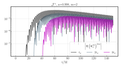
In Fig. 2 we plot the absolute value of the real and imaginary parts of $\Psi_{4}^{(1),[m]}$ , along with $\Psi_{4}^{(2),[2m]}$ and $\Psi_{4}^{(2),[0]}$ , measured at future null infinity. The time offset between the start of the first and second order components of the waveform is due to the delayed integration start time $T_{w}$ of the latter compared to the former; $T=T_{w}$ is twice the earliest time we can begin the second order evolution with a consistent source term. In Fig. 3 we plot the absolute value of the real and imaginary parts of $\Psi_{4}^{(1)}$ and $\mathcal{S}^{(2)}$ on the black hole horizon; Fig. 4 shows a resolution study of the latter. The region near the horizon is where the source term is most significant (it decays faster than $1/r$ going to null infinity), and as expected $\mathcal{S}^{(2)}\sim\left(\Psi_{4}^{(1)}\right)^{2}$ there. In Fig. 5 we plot norms of the metric reconstruction independent residuals discussed in Sec.V.8, at three different resolutions. After the constraint violating portions have left the domain, we find roughly exponential convergence to zero, in agreement with what one would expect from a pseudo-spectral code with a sufficiently small time step so that the time integration truncation error is subdominant.

Though this initial data is more to illustrate our solution scheme and is not astrophysically accurate, it is useful to begin to understand the non-linear response when the black hole is excited by the fundamental $l=m=2$ quasinormal mode, in particular if we wait a sufficiently long time for overtones present in the initial data to decay⁸⁸8In a Kerr spacetime, setting initial data (38) with a single $l_{0}$ mode of the spin-weighted Legendre polynomials ${}_{s}P^{m}_{l_{0}}$ will excite a spectrum of different $l$ quasinormal modes measured at infinity, unless the black hole spin $a=0$ .. Fig. 2 suggests $T=T_{w}$ might not be early enough, as $\Psi_{4}^{(1)}$ has just started to enter its decaying phase. In Fig. 6 then we show results for the second order modes with the evolution begun at $2T_{w}$ and $3T_{w}$ , in addition to $T_{w}$ depicted in Fig. 2. The later start times show qualitatively similar behavior, except the amplitude is lower by a factor close to the square of the decay in the amplitude of $\Psi_{4}^{(1)}$ over the relevant delay time. To help interpret the results further, in Fig. 7 we plot the normalized absolute value of the Fourier transform of $\Psi_{4}$ , taken with two different windows: an earlier time window to capture the prompt second order response (but still sufficiently past $T=0$ that the first order source is dominated by the single decaying quasinormal mode), and a later time window to show the late time behavior once second order transient effects have decayed. Also shown for reference are Fourier transforms of pure damped sinusoids corresponding to the dominant fundamental quasinormal modes expected for each $m$ .

These plots illustrate a couple of interesting aspects of the second order piece of a quasinormal mode perturbation of an $a=0.7$ spin Kerr black hole. First, beginning with zero initial data for $\Psi_{4}^{(2)}$ on our $T={\rm const.}$ slice, the response at future null infinity builds up to a maximum over 1-2 local dynamical times scales, before settling down to a quasinormal mode-like decay. This is in part because where the source term is most significant is spread out over a region a few Schwarzschild radii about the horizon, and in part because of our prompt start of the second order evolution. Second, the source term clearly excites the fundamental $m=0$ and $m=4$ quasinormal modes (i.e. solutions one would obtain from the source-free Teukolsky equation), and these dominate the late time response due to their slower decay. Or said another way, suppose the late time response was purely a driven mode, then (following the behavior of the source term in Fig. 3) one would expect the slope to be twice that of the first order mode, and the amplitude of the second order piece at a given late-time should not depend on the start time, unlike what is shown in Figs. 2 and 6.⁹⁹9All this behavior can qualitatively be captured by a driven, damped harmonic oscillator model, $d^{2}y(t)/dt^{2}+\lambda\ dy(t)/dt+\omega^{2}\ y(t)=f(t)$ , where the source $f(t)$ is zero before being turned on at time $t_{0}$ . In addition to the driven (particular solution) response to $f(t)$ , demanding continuity in $y$ and $dy/dt$ at $t=t_{0}$ will generically require that the fundamental modes (homogeneous solutions) of the oscillator are also excited then. From the perspective of the Fourier transforms in Fig. 7, for $m=4$ the presence of this early time behavior can be inferred by the narrower shape of the numerical data curve compared to that of the fundamental quasinormal mode: the driven and fundamental modes have essentially the same frequency to within the resolution of the Fourier transform here, and despite the more rapid decay of the former, the initial growth phase (Fig. 6) makes the transform of their sum look slightly closer to that of an undamped sinusoid (a delta function). The interpretation of the $m=0$ mode in this sense is less clear.

An implication of the above for ringdown studies are (caveats about the physical accuracy of our initial data aside): if an $l=m=4$ component is searched for following a comparable mass merger, given this mode’s low amplitude relative to the $l=m=2$ mode, in the first few cycles of ringdown non-linear energy transfer from the $l=m=2$ to the $l=m=4$ mode could be observable and should be accounted for. Furthermore, once past this and in the linear regime, the amplitude and phase of the $l=m=4$ mode that may be measured then would differ from the linear evolution of what one could consider as the “initial” amplitude and phase of this mode excited by merger. With proposals to coherently stack multiple detected events to search for common subdominant modes that rely on knowledge of predicted amplitudes and phases Yang et al. (2017), this implies non-linear effects need to be accounted for, either by incorporating them in the models, or using the “final” amplitudes and phases if only the linear portion of the waveforms are included.

VI.2 Example evolution with black hole spin $a=0.998$

Here we show results from a simulation of the perturbation of a black hole with a spin near the “Thorne limit” Thorne (1974) $a\sim 0.998$ , which is expected to be the maximum black hole spin that can be achieved within a class of thin-disk accretion models. Our simulation parameters are listed in Table. 4. Note that the relevant dynamical timescale for a near extremal black hole is $T_{d}\sim M/\sqrt{1-a}$ . For $a=0.998$ , $T_{d}\sim 22M$ , so evolving for $T\sim 150M$ corresponds to $T\sim 7\times T_{d}$ , a considerably shorter time in terms of $T_{d}$ than for $a=0.7$ . Given that it is computationally intensive to evolve the $a=0.998$ case for a comparable number of dynamical timescales with our present code, we leave investigating late time effects to future work.

mass	$0.5$
spin	$0.499$ ( $a=0.998$ )
low resolution	$N_{x}=176$ , $N_{l}=32$
med resolution	$N_{x}=192$ , $N_{l}=36$
high resolution	$N_{x}=208$ , $N_{l}=40$
$T_{w}$	$2\times T_{mw}\approx 13.6M$
$m$	$-2$
$l_{0}$	$2$
$a_{0}$	$0.1$
$r_{u}$	$1.1\times r_{H}$
$r_{l}$	$2.5\times r_{H}$

Table 4: Parameters for spin

a=0.998

black hole evolution (unless stated otherwise in the figure captions).

T_{w}

is the “wait” time before starting the evolution of

\Psi_{4}^{(2)}

, which we choose to be twice the “minimum” wait time

T_{mw}

for the initial data we choose; see Sec. (IV).

We show the same set of data as from the $a=0.7$ runs : the magnitudes of $\Psi_{4}^{(1)}$ and $\Psi_{4}^{(2)}$ at future null infinity (Fig.8), the magnitudes of $\Psi_{4}^{(1)}$ and $\mathcal{S}^{(2)}$ at the horizon (Fig.9), a resolution study of the latter (Fig. 10), convergence of the metric reconstruction independent residuals (Fig.11), the second order response with varied start time (Fig.12), and Fourier transforms of $\Psi_{4}^{(1)}$ and $\Psi_{4}^{(2)}$ at future null infinity (Fig.13).

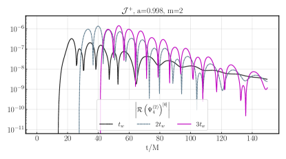
For the most part the interpretation of the results is similar to the $a=0.7$ case, taking into account the shorter evolution time in terms of $T_{d}$ for the $a=0.998$ case. A notable difference though is a significant non-oscillatory component to the second order $m=0$ mode. One can roughly understand why such a component might appear given our initial data for $\Psi_{4}^{(1),[m]}\propto e^{i\omega_{R}t-\omega_{I}t}$ (we follow the quasinormal mode convention where an exponential $e^{i\omega t}$ has complex frequency $\omega\equiv\omega_{R}+i\omega_{I}$ ). The $m=0$ source term largely comes form reconstructed fields of the form $p^{[m]}\times\overline{q^{[m]}}$ , where $p^{[m]},q^{[m]}\propto\Psi_{4}^{(1),[m]}$ ; hence their oscillatory components can cancel, leaving a real exponential piece decaying at roughly twice the rate of $\Psi_{4}^{(1),[m]}$ . For near extremal spins (in contrast to the $a=0.7$ case), this driven component has a decay rate quite close to the fundamental $m=0,l=2$ harmonic ¹⁰¹⁰10See e.g. Table II of Berti et al. (2006) for their $a=0.98$ case, the closest spin to our value that they list., which is why it remains visible in the waveform at late times. We find that how much of an oscillatory vs pure exponential piece is visible in either of the real or imaginary parts of $\Psi_{4}^{(2),[0]}$ depends quite sensitively on the relative amplitudes and phases of the real vs imaginary components of $\Psi_{4}^{(1)}$ in the initial data.

VII Conclusion and further extensions

We have presented a new numerical evolution scheme to reconstruct the linear metric from the Weyl scalar $\Psi_{4}^{(1)}$ in Kerr spacetimes, along with a numerical implementation of the equations of motion for the second order perturbation $\Psi_{4}^{(2)}$ (a more detailed discussion of the analytic framework we used is discussed in the Appendices of this paper, and in our first paper Loutrel et al. (2020)). This first implementation is limited in several respects, and in the remainder of this section we outline possible extensions that will allow more direct application to our desired goals of studying second order effects in post-merger black hole ringdown, investigating gravitational wave turbulence, and other related issues for rapidly rotating Kerr black holes.

In this study we only considered mode coupling from a single mode of angular number $m$ , $\Psi_{4}^{(1),[m]}$ , to produce the frequency doubled second order components $\Psi_{4}^{(2),[2m]}$ and $\Psi_{4}^{(2),[0]}$ . Astrophysically realistic sets of initial data will include many different modes, and the second order perturbations for an $m$ mode will be a sum over all modes $(m_{1},m_{2})$ such that $m_{1}+m_{2}=m$ . We leave exploring such more complicated mode mixing to future work.

Constructing astrophysically realistic initial data for $\Psi_{4}^{(1)}$ , and the $l=0,1$ components of the metric and NP scalars that represent the changes in mass and spin corresponding to the given $\Psi_{4}^{(1)}$ , remain unsolved problems in black hole perturbation theory. This will require specifying a $\Psi_{4}^{(1)}$ that matches a desired scenario at $T=0$ , and then solving a set of constraint equations to give consistent initial conditions (perturbed metric and related NP quantities) for the reconstruction transport equations. These constraint equations are most naturally expressed in terms of geometric quantities intrinsic to the spacelike hypersurface $T=0$ , giving rise to the familiar Hamiltonian and momentum contraint equations. One approach to take could be based on solving these equations using established approaches Baumgarte and Shapiro (2010), and then transforming the solutions to initial conditions for our scheme. Following a merger, finding appropriate values of $\Psi_{4}^{(1)}$ (or equivalently choosing the free initial data for $h_{\mu\nu}$ in a traditional scheme) describing the perturbation of the remnant, is less well understood. One possible approach to tackle this is to follow the lines of earlier analytical studies, including the close limit approximation to comparable mass black hole mergers Price and Pullin (1994), or related work done for the EMRI problem Apte and Hughes (2019); Lim et al. (2019). Another approach might be to map the data from a constant time slice of a full numerical simulation to our coordinates, and try to extract a perturbation relative to the late time Kerr solution. (And we note that, as discussed in more detail in the companion paper Loutrel et al. (2020), our goal is not to simply “solve” for the post merger waveform to second order; numerical relativity can already give us the full nonlinear solution as accurately as computer resources allow. Rather, we want to be able to interpret ringdown studies in terms of quasinormal modes, which requires understanding the waveform at a quantitative level that the full “answer”, in terms of a waveform by itself, cannot give.)

Another area of future work we mention is to investigate whether one can adapt our scheme to a gauge condition that is less restrictive on matter/effective matter in the spacetime than the outgoing radiation gauge. For at present we cannot study (for example) the EMRI problem, where there is a matter source representing the small body, and we cannot reconstruct the second order metric corresponding to the second order piece of $\Psi_{4}$ . To list two potential ways forward, it may be possible to continue to work in a radiation gauge but evolve a “corrector tensor” to include matter fields as in Green et al. (2020), or to directly reconstruct the metric in a different gauge, as is done in Chandrasekhar (2002); Andersson et al. (2019).

We emphasize that we have implemented a form of “ordinary” perturbation theory (e.g. Bender and Orszag (2013)), based on expansion in the curvature (or equivalently the peturbed metric)

\displaystyle\Psi_{4}=\Psi_{4}^{(1)}+\Psi_{4}^{(2)}+\cdots,

(45)

where the corrections are solved order-by-order, and at each order the new correction is assumed smaller than the prior sum. Up to second order then, the only non-linear phenomena we can explore is mode-coupling. We mentioned one of our goals was to understand whether Kerr black holes could exhibit “turbulence”, though exactly what turbulence means in the case of black holes is a bit nebulous. Regardless, the authors of Yang et al. (2015); Green et al. (2014) who first suggested turbulence could be present in the 4D case argued it would be a more subtle effect than can be described by ordinary perturbation theory, or at least would require some “resumming” of many terms in the sum. Instead then, they proposed an alternative perturbative expansion to try to capture such effects at leading beyond-linear order, showing in a scalar field model that a kind of parametric instability resulted that might be able to drive a turbulent cascade. It is still unknown whether such an effect occurs for gravitational perturbations of Kerr, though mode coupling more along the lines of what we describe here has been seen in full numerical solutions of both perturbed 4D Kerr black holes East et al. (2014) and black holes in 5D AdS spacetime Bantilan et al. (2012). We leave it to future work for a more thorough comparison with full numerical results, as well as how close second order mode coupling, augmented with energy transfer between modes guided by measurements at null infinity mentioned in Sec. III, could come to describing a turbulent-like cascade of energy for rapidly spinning black holes.

Acknowledgements

We are grateful to Andrew Spiers and Adam Pound for sharing results of their calculations which confirmed our calculation of Eq. (51) (and which confirmed several errors in Eq. (A4) of Campanelli and Lousto (1999)), to Stefan Hollands for discussions on the metric reconstruction method described in Green et al. (2020), and to Scott Hughes and Richard Price for a helpful discussion on our project and earlier work on second order black hole perturbation theory. N.L. & F.P. acknowledge support from NSF grant PHY-1912171, the Simons Foundation, and the Canadian Institute for Advanced Research (CIFAR). E.G. acknowledges support from NSF grant DMS-2006741. The simulations presented in this article were performed on computational resources managed and supported by Princeton Research Computing, a consortium of groups including the Princeton Institute for Computational Science and Engineering (PICSciE) and the Office of Information Technology’s High Performance Computing Center and Visualization Laboratory at Princeton University.

Appendix A Conventions for discrete norms and Fourier transforms

As fields are typically complex in the NP formalism, the discrete two norm of a field $f$ at a time level $n$ is defined to be the sum

$\displaystyle\|f(t_{n})\|_{2}\equiv$
$\displaystyle\bigg{(}\frac{1}{N_{x}N_{y}}\sum_{i=1}^{N_{x}}\sum_{j=1}^{N_{y}}\big{(}$	$\displaystyle\left(\mathcal{R}f(t_{n},r_{i},\vartheta_{j})\right)^{2}$
	$\displaystyle+\left(\mathcal{I}f(t_{n},r_{i},\vartheta_{j})\right)^{2}\big{)}\bigg{)}^{1/2}.$	(46)

Our conventions for the Fourier transform are

	$\displaystyle\hat{f}(\omega)=\int_{-\infty}^{\infty}dte^{-i\omega t}f(t),$
	$\displaystyle f(t)=\int_{-\infty}^{\infty}\frac{d\omega}{2\pi}e^{i\omega t}\hat{f}(\omega).$		(47)

And we define a normalized Fourier transform by

\displaystyle\mathcal{N}\hat{f}(\omega)\equiv\frac{1}{\mathrm{max}\hat{f}}|\hat{f}(\omega)|.

(48)

For reference the absolute value of the Fourier transform of $f(t)=\Theta(t)e^{-\omega_{I}t}\mathrm{sin}\left(\omega_{R}t\right)$ is

\displaystyle\left|\hat{f}(\omega)\right|=\frac{\omega_{R}}{\sqrt{\left(\omega_{R}^{2}+\omega_{I}^{2}-\omega^{2}\right)^{2}+4\omega_{I}^{2}\omega^{2}}}.

(49)

Appendix B Derivation of metric reconstruction equations and source term in the outgoing radiation gauge

B.1 Tetrad, gauge, and first order spin coefficients

We assume the background is type D, that the background tetrad has been chosen to set $\Psi_{0}=\Psi_{1}=\Psi_{3}=\Psi_{4}=\kappa=\sigma=\nu=\lambda=0$ , the linearized tetrad is as in (11a), and we are using outgoing radiation gauge for the first order metric perturbation (9a). For the Kerr spacetime we can also rotate the background tetrad to set $\gamma=0$ (see Sec. C), and we assume we have done this.

It is worth noting that the tetrad components of the metric perturbation (10a) are all scalars of definite spin and boost weight, which we catalogue in Table 5 (for the angular tetrad projections we list the spin and boost of their complex conjugates, which is what we mostly use).

scalar	weight	spin weight	boost weight
$h_{ll}$	$\{2,2\}$	$0$	$2$
$h_{l\bar{m}}$	$\{0,2\}$	$-1$	$1$
$h_{\bar{m}\bar{m}}$	$\{-2,2\}$	$-2$	$0$

Table 5: Nonzero contractions of the perturbed metric.

We can write the first order perturbed tetrad in terms of the background tetrad. Following Chrzanowski (1976) (see also Campanelli and Lousto (1999); Loutrel et al. (2020)) we have


$\displaystyle l^{(1)}_{\mu}=$	$\displaystyle\frac{1}{2}h_{ll}n_{\mu},$	(50a)
$\displaystyle n^{(1)}_{\mu}=$	$\displaystyle 0,$	(50b)
$\displaystyle m^{(1)}_{\mu}=$	$\displaystyle h_{lm}n_{\mu}-\frac{1}{2}h_{mm}\bar{m}_{\mu},$	(50c)

which then immediately gives the expressions for the perturbed derivative operators listed in (11a).

With the above choices for the tetrad/gauge, we find the following first order corrections to the spin coefficients (for the more general version of these expressions, without the choice of ingoing radiation gauge and $\gamma=0$ , see Loutrel et al. (2020)):


$\displaystyle\kappa^{(1)}=$	$\displaystyle\left(D-2\epsilon-\bar{\rho}\right)h_{lm}$
	$\displaystyle-\frac{1}{2}\left(\delta-2\bar{\alpha}-2\beta+\bar{\pi}+\tau\right)h_{ll},$	(51a)
$\displaystyle\lambda^{(1)}=$	$\displaystyle-\frac{1}{2}\left(\Delta-\mu+\bar{\mu}\right)h_{\bar{m}\bar{m}},$	(51b)
$\displaystyle\sigma^{(1)}=$	$\displaystyle\frac{1}{2}\left(D-2\epsilon+2\bar{\epsilon}+\rho-\bar{\rho}\right)h_{mm}$
	$\displaystyle-\left(\bar{\pi}+\tau\right)h_{lm},$	(51c)
$\displaystyle\epsilon^{(1)}=$	$\displaystyle-\frac{1}{4}\left(\Delta-\mu+\bar{\mu}\right)h_{ll}$
	$\displaystyle-\frac{1}{4}\left(\delta-2\bar{\alpha}+\bar{\pi}+2\tau\right)h_{l\bar{m}}$
	$\displaystyle+\frac{1}{4}\left(\bar{\delta}-2\alpha-3\pi-2\bar{\tau}\right)h_{lm},$	(51d)
$\displaystyle\rho^{(1)}$	$\displaystyle=\frac{1}{2}\mu h_{ll}+\frac{1}{2}\left(\bar{\delta}-2\alpha-\pi\right)h_{lm}$
	$\displaystyle-\frac{1}{2}\left(\delta-2\bar{\alpha}+\bar{\pi}+2\tau\right)h_{l\bar{m}},$	(51e)
$\displaystyle\alpha^{(1)}=$	$\displaystyle-\frac{1}{4}\left(\Delta-2\mu+\bar{\mu}\right)h_{l\bar{m}}$
	$\displaystyle-\frac{1}{4}\left(\delta-2\bar{\alpha}+\bar{\pi}+\tau\right)h_{\bar{m}\bar{m}},$	(51f)
$\displaystyle\beta^{(1)}=$	$\displaystyle-\frac{1}{4}\left(\Delta+\mu+2\bar{\mu}\right)h_{lm}$
	$\displaystyle+\frac{1}{4}\left(\bar{\delta}+2\bar{\beta}-\pi-\bar{\tau}\right)h_{mm},$	(51g)
$\displaystyle\pi^{(1)}=$	$\displaystyle-\frac{1}{2}\left(\Delta+\bar{\mu}\right)h_{l\bar{m}}-\frac{1}{2}\tau h_{\bar{m}\bar{m}},$	(51h)
$\displaystyle\tau^{(1)}=$	$\displaystyle\frac{1}{2}\left(\Delta+\mu\right)h_{lm}-\frac{1}{2}\pi h_{mm}.$	(51i)

The following perturbed NP scalars are zero

\displaystyle\nu^{(1)}=\gamma^{(1)}=\mu^{(1)}=0.

(52)

Notice that

\displaystyle\pi^{(1)}+\bar{\tau}^{(1)}=

\displaystyle-\frac{1}{2}\left(\bar{\pi}+\tau\right)h_{\bar{m}\bar{m}}.

(53)

so it is straightforward to find, e.g. $\bar{\tau}^{(1)}$ once we know $\pi^{(1)}$ and $h_{\bar{m}\bar{m}}$ .

B.2 Reconstructing the metric from $\Psi_{4}^{(1)}$

Here we list the sequence of step we use to reconstruct all the metric coefficients $h_{ll}$ , $h_{l\bar{m}}$ , and $h_{\bar{m}\bar{m}}$ from the curvature component $\Psi_{4}^{(1)}$ .

With $\Psi_{4}^{(1)}$ one can find $\Psi_{3}^{(1)}$ and $\lambda^{(1)}$ . We begin with the following Bianchi identity (Eq. (1.321.h) in Chandrasekhar (2002)):

		$\displaystyle 3\nu\Psi_{2}-2\left(\gamma+2\mu\right)\Psi_{3}$
		$\displaystyle+\left(4\beta-\tau\right)\Psi_{4}+\delta\left(\Psi_{4}\right)-\Delta\left(\Psi_{3}\right)=0;$		(54)

linearizing this gives

		$\displaystyle 3\nu^{(1)}\Psi_{2}-4\mu\Psi_{3}^{(1)}$
		$\displaystyle+\left(4\beta-\tau\right)\Psi_{4}^{(1)}+\delta\Psi_{4}^{(1)}-\Delta\Psi_{3}^{(1)}=0.$		(55)

Using the gauge condition (52) and writing out the NP $\{\delta,\bar{\delta}\}$ derivatives in terms of the GHP derivatives $\{\textnormal{\dh},\textnormal{\dh}^{\prime}\}$ , i.e. $\textnormal{\dh}\Psi_{4}^{(1)}=(\delta+4\beta)\Psi_{4}^{(1)}$ , we obtain

\displaystyle\left(\textnormal{\dh}-\tau\right)\Psi_{4}^{(1)}-\left(\Delta+4\mu\right)\Psi_{3}^{(1)}=

\displaystyle 0.

(56)

The above is a first order differential equation for $\Psi_{3}^{(1)}$ in terms of the known $\Psi_{4}^{(1)}$ . Similarly, the linearization of

		$\displaystyle\lambda\left(3\gamma-\bar{\gamma}+\mu+\bar{\mu}\right)-\nu\left(3\alpha+\bar{\beta}+\pi-\bar{\tau}\right)$
		$\displaystyle+\Psi_{4}+\Delta\left(\lambda\right)-\bar{\delta}\left(\nu\right)=0$		(57)

(Eq. (1.310.j) in Chandrasekhar (2002)) gives

\displaystyle-\Psi_{4}^{(1)}-\left(\Delta+\mu+\bar{\mu}\right)\lambda^{(1)}=

\displaystyle 0,

(58)

a differential equation for $\lambda^{(1)}$ .

With $\Psi_{3}^{(1)}$ we can find $\Psi_{2}^{(1)}$ . The linearization of

		$\displaystyle 2\nu\Psi_{1}-3\mu\Psi_{2}+2\beta\Psi_{3}-2\tau\Psi_{3}$
		$\displaystyle+\sigma\Psi_{4}+\delta\left(\Psi_{3}\right)-\Delta\left(\Psi_{2}\right)=0$		(59)

(Eq. (1.321.g) of Chandrasekhar (2002)) gives

		$\displaystyle-3\mu\Psi_{2}^{(1)}+2\beta\Psi_{3}^{(1)}-2\tau\Psi_{3}^{(1)}$
		$\displaystyle+\sigma\Psi_{4}^{(1)}+\delta\Psi_{3}^{(1)}-\Delta\Psi_{2}^{(1)}=0.$		(60)

By using $\textnormal{\dh}\Psi_{3}^{(1)}=(\delta+2\beta)\Psi_{3}^{(1)}$ , we obtain the desired differential equation for $\Psi_{2}^{(1)}$ :

\displaystyle\left(\textnormal{\dh}-2\tau\right)\Psi_{3}^{(1)}-\left(\Delta+3\mu\right)\Psi_{2}^{(1)}=

\displaystyle 0.

(61)

3.

With $\lambda^{(1)}$ we can now solve for $h_{\bar{m}\bar{m}}$ using (51b).

With $\lambda^{(1)}$ , $h_{\bar{m}\bar{m}}$ , and $\Psi_{3}^{(1)}$ we can find $\pi^{(1)}$ . Using the linearization of

		$\displaystyle\left(3\epsilon+\bar{\epsilon}\right)\nu-\gamma\pi+\bar{\gamma}\pi-\lambda\left(\bar{\pi}+\tau\right)$
		$\displaystyle-\mu\left(\pi+\bar{\tau}\right)-\Psi_{3}+D\left(\nu\right)-\Delta\left(\pi\right)=0,$		(62)

(Eq. (1.310.i) of Chandrasekhar (2002)) namely,

	$\displaystyle\ \ \ -$	$\displaystyle\lambda^{(1)}\left(\bar{\pi}+\tau\right)-\mu\left(\pi+\bar{\tau}\right)^{(1)}$
		$\displaystyle-\Psi_{3}^{(1)}-\Delta\pi^{(1)}=0,$		(63)

and using (53) gives the differential equation to solve for $\pi^{(1)}$ :

	$\displaystyle\ \ \ -$	$\displaystyle\lambda^{(1)}\left(\bar{\pi}+\tau\right)+\frac{1}{2}\mu\left(\bar{\pi}+\tau\right)h_{\bar{m}\bar{m}}$
		$\displaystyle-\Psi_{3}^{(1)}-\Delta\pi^{(1)}=0.$		(64)

5.

With $\pi^{(1)}$ and $h_{\bar{m}\bar{m}}$ we can solve for $h_{l\bar{m}}$ using (51h).

With $\Psi_{2}^{(1)}$ , $h_{lm}$ and $h_{mm}$ we can find $h_{ll}$ . The linearization of

	$\displaystyle\Psi_{2}=$	$\displaystyle\epsilon\mu+\bar{\epsilon}\mu+\kappa\nu+\bar{\alpha}\pi-\beta\pi-\pi\bar{\pi}$
		$\displaystyle-\mu\bar{\rho}-\lambda\sigma+D\left(\mu\right)-\delta\left(\pi\right),$		(65)

(Eq. (1.310.h) of Chandrasekhar (2002)) gives

$\displaystyle\Psi_{2}^{(1)}=$	$\displaystyle(\epsilon^{(1)}+\bar{\epsilon}^{(1)})\mu+\left(\bar{\alpha}^{(1)}-\beta^{(1)}\right)\pi$
	$\displaystyle+\left(-\delta+\bar{\alpha}-\beta-\bar{\pi}\right)\pi^{(1)}-\pi\bar{\pi}^{(1)}$
	$\displaystyle-\mu\bar{\rho}^{(1)}-\frac{1}{2}h_{ll}\Delta\left(\mu\right)$
	$\displaystyle+\left(h_{lm}\Delta-\frac{1}{2}h_{mm}\bar{\delta}\right)\left(\pi\right),$	(66)

where we used (11a). From (51), we deduce

	$\displaystyle\epsilon^{(1)}+\bar{\epsilon}^{(1)}$	$\displaystyle=-\frac{1}{2}\Delta h_{ll}-\left(\bar{\pi}+\tau\right)h_{l\bar{m}}$
		$\displaystyle-\left(\pi+\bar{\tau}\right)h_{lm}$		(67)

and from (51), we find

	$\displaystyle\bar{\rho}^{(1)}$	$\displaystyle=\frac{1}{2}\bar{\mu}h_{ll}+\frac{1}{2}\left(\textnormal{\dh}-\bar{\pi}\right)h_{l\bar{m}}$
		$\displaystyle-\frac{1}{2}\left(\textnormal{\dh}^{\prime}+\pi+2\bar{\tau}\right)h_{lm},$		(68)

where we have used $\textnormal{\dh}h_{l\bar{m}}=(\delta-2\bar{\alpha})h_{l\bar{m}}$ and $\textnormal{\dh}^{\prime}h_{lm}=(\bar{\delta}-2\alpha)h_{lm}$ .

From (51) and (51), we obtain

	$\displaystyle\bar{\alpha}^{(1)}-\beta^{(1)}$	$\displaystyle=\bar{\mu}h_{lm}$
		$\displaystyle-\frac{1}{2}\left(\textnormal{\dh}^{\prime}+\alpha-\bar{\beta}\right)h_{mm},$		(69)

where we have used $\textnormal{\dh}^{\prime}h_{mm}=(\bar{\delta}+2\bar{\beta}-2\alpha)h_{mm}$ .

Substituting the above in (6) gives

$\displaystyle\ \ \ \ \Psi_{2}^{(1)}$	$\displaystyle=\bigg{(}-\frac{1}{2}\Delta h_{ll}-\left(\bar{\pi}+\tau\right)h_{l\bar{m}}-\left(\pi+\bar{\tau}\right)h_{lm}\bigg{)}\mu$
	$\displaystyle+\left(\bar{\mu}h_{lm}-\frac{1}{2}\left(\textnormal{\dh}^{\prime}+\alpha-\bar{\beta}\right)h_{mm}\right)\pi$
	$\displaystyle+\left(-\textnormal{\dh}-\bar{\pi}\right)\pi^{(1)}-\pi\bar{\pi}^{(1)}$
	$\displaystyle-\mu\bigg{(}\frac{1}{2}\bar{\mu}h_{ll}+\frac{1}{2}\left(\textnormal{\dh}-\bar{\pi}\right)h_{l\bar{m}}$
	$\displaystyle-\frac{1}{2}\left(\textnormal{\dh}^{\prime}+\pi+2\bar{\tau}\bigg{)}h_{lm}\right)-\frac{1}{2}h_{ll}\Delta\left(\mu\right)$
	$\displaystyle+\left(h_{lm}\Delta-\frac{1}{2}h_{mm}\left(\textnormal{\dh}^{\prime}-\alpha+\bar{\beta}\right)\right)\left(\pi\right)$	(70)

which we rewrite as

	$\displaystyle-\frac{1}{2}\left(\Delta+\bar{\mu}\right)\left(\mu h_{ll}\right)-\frac{1}{2}\mu\left(\textnormal{\dh}+\bar{\pi}+2\tau\right)h_{l\bar{m}}$
	$\displaystyle+\frac{1}{2}\left(\mu\left(\textnormal{\dh}^{\prime}-\pi\right)+2\bar{\mu}\pi\right)h_{lm}$
	$\displaystyle-\frac{1}{2}\pi\textnormal{\dh}^{\prime}h_{mm}-\left(\textnormal{\dh}+\bar{\pi}\right)\pi^{(1)}-\pi\bar{\pi}^{(1)}$
	$\displaystyle+h_{lm}\Delta\pi-\frac{1}{2}h_{mm}\textnormal{\dh}^{\prime}\pi-\Psi_{2}^{(1)}=0.$		(71)

Using (62), and Eq. (1.310.g) in Chandrasekhar (2002),

		$\displaystyle 3\epsilon\lambda+\bar{\kappa}\nu-\pi\left(\alpha-\bar{\beta}+\pi\right)-\lambda\left(\bar{\epsilon}+\rho\right)$
		$\displaystyle-\mu\bar{\sigma}+D\left(\lambda\right)-\bar{\delta}\left(\pi\right)=0,$		(72)

evaluated on a type D background ( $\gamma=0$ ) to write

\displaystyle\ \ \ \Delta\left(\pi\right)=-\mu\left(\pi+\bar{\tau}\right),\,\,\,\,\textnormal{\dh}^{\prime}\left(\pi\right)=-\pi\pi,

(73)

we finally obtain the transport equation for $h_{ll}$

	$\displaystyle-\left(\Delta+\bar{\mu}\right)\left(\mu h_{ll}\right)-\mu\left(\textnormal{\dh}+\bar{\pi}+2\tau\right)h_{l\bar{m}}+$
	$\displaystyle\left(\mu\left(\textnormal{\dh}^{\prime}-3\pi-2\bar{\tau}\right)+2\bar{\mu}\pi\right)h_{lm}$
	$\displaystyle-\pi\left(\textnormal{\dh}^{\prime}-\pi\right)h_{mm}-2\left(\textnormal{\dh}+\bar{\pi}\right)\pi^{(1)}$
	$\displaystyle-2\pi\bar{\pi}^{(1)}-2\Psi_{2}^{(1)}=0.$		(74)

With $\{h_{ll},h_{l\bar{m}},h_{\bar{m}\bar{m}}\}$ one can readily compute the rest of the NP scalars in outgoing radiation gauge, and we are now able to compute the second order source term.

B.3 Source term for $\Psi_{4}^{(2)}$

In this section we rewrite the vacuum source term $\mathcal{S}^{(2)}$ for the Teukolsky equation for $\Psi_{4}^{(2)}$ Campanelli and Lousto (1999),

		$\displaystyle\ \ \ \mathcal{S}^{(2)}\equiv$
		$\displaystyle-\bigg{[}d_{4}\left(D+4\epsilon-\rho\right)^{(1)}-d_{3}\left(\delta+4\beta-\tau\right)^{(1)}\bigg{]}\Psi_{4}^{(1)}$
		$\displaystyle+\bigg{[}d_{4}\left(\bar{\delta}+2\alpha+4\pi\right)^{(1)}-d_{3}\left(\Delta+2\gamma+4\mu\right)^{(1)}\bigg{]}\Psi_{3}^{(1)}$
		$\displaystyle-3\left[d_{4}\lambda^{(1)}-d_{3}\nu^{(1)}\right]\Psi^{(1)}_{2}$
		$\displaystyle+3\Psi^{(0)}_{2}\bigg{[}\left(d^{(1)}_{4}-3\mu^{(1)}\right)\lambda^{(1)}-\left(d^{(1)}_{3}-3\pi^{(1)}\right)\nu^{(1)}\bigg{]},$		(75)

in outgoing radiation gauge, with a tetrad chosen so that $\gamma=0$ . In the above we have introduced the background operators


	$\displaystyle d_{3}\equiv$	$\displaystyle\bar{\delta}+3\alpha+\bar{\beta}+4\pi-\bar{\tau},$	(76a)
	$\displaystyle d_{4}\equiv$	$\displaystyle\Delta+4\mu+\bar{\mu},$	(76b)
and their first order corrections

	$\displaystyle d_{3}^{(1)}\equiv$	$\displaystyle\bar{\delta}^{(1)}+3\alpha^{(1)}+\bar{\beta}^{(1)}+4\pi^{(1)}-\bar{\tau}^{(1)},$	(76c)
	$\displaystyle d_{4}^{(1)}\equiv$	$\displaystyle 0.$	(76d)

We now consider the expansion of $\mathcal{S}^{(2)}$ line by line.

The first line is

\displaystyle-\left[d_{4}\left(D+4\epsilon-\rho\right)^{(1)}-d_{3}\left(\delta+4\beta-\tau\right)^{(1)}\right]\Psi_{4}^{(1)}.

(77)

By using (51), we expand

	$\displaystyle\left(D+4\epsilon-\rho\right)^{(1)}\Psi_{4}^{(1)}$
	$\displaystyle=\Big{(}-\frac{1}{2}h_{ll}\Delta-\left(\Delta-\mu+\bar{\mu}\right)h_{ll}$
	$\displaystyle-\left(\delta-2\bar{\alpha}+\bar{\pi}+2\tau\right)h_{l\bar{m}}$
	$\displaystyle+\left(\bar{\delta}-2\alpha-3\pi-2\bar{\tau}\right)h_{lm}-\rho^{(1)}\Big{)}\Psi_{4}^{(1)}$
	$\displaystyle=-\frac{1}{2}h_{ll}\Delta\Psi_{4}^{(1)}-\Psi_{4}^{(1)}\left(\Delta-\mu+\bar{\mu}\right)h_{ll}$
	$\displaystyle-\Psi_{4}^{(1)}\left(\textnormal{\dh}+\bar{\pi}+2\tau\right)h_{l\bar{m}}$
	$\displaystyle+\Psi_{4}^{(1)}\left(\textnormal{\dh}^{\prime}-3\pi-2\bar{\tau}\right)h_{lm}-\Psi_{4}^{(1)}\rho^{(1)}.$		(78)

By using (51) and (53), we expand

		$\displaystyle\left(\delta+4\beta-\tau\right)^{(1)}\Psi_{4}^{(1)}$
		$\displaystyle=\Big{(}-h_{lm}\Delta+\frac{1}{2}h_{mm}\bar{\delta}-\left(\Delta+\mu+2\bar{\mu}\right)h_{lm}$
		$\displaystyle+\left(\bar{\delta}+2\bar{\beta}-\pi-\bar{\tau}\right)h_{mm}+\bar{\pi}^{(1)}+\frac{1}{2}(\pi+\bar{\tau})h_{mm}\Big{)}\Psi_{4}^{(1)}$
		$\displaystyle=-h_{lm}\Delta\Psi_{4}^{(1)}+\frac{1}{2}h_{mm}\bar{\delta}\Psi_{4}^{(1)}$
		$\displaystyle+\Psi_{4}^{(1)}\bigg{[}-\left(\Delta+\mu+2\bar{\mu}\right)h_{lm}+\left(\bar{\delta}+2\bar{\beta}-\pi-\bar{\tau}\right)h_{mm}$
		$\displaystyle+\bar{\pi}^{(1)}+\frac{1}{2}(\pi+\bar{\tau})h_{mm}\bigg{]}$
		$\displaystyle=-h_{lm}\left(\Delta+\mu+2\bar{\mu}\right)\Psi_{4}^{(1)}+\frac{1}{2}h_{mm}\textnormal{\dh}^{\prime}\Psi_{4}^{(1)}$
		$\displaystyle+\Psi_{4}^{(1)}\bigg{[}-\Delta h_{lm}+\left(\textnormal{\dh}^{\prime}-\frac{1}{2}\pi-\frac{1}{2}\bar{\tau}\right)h_{mm}+\bar{\pi}^{(1)}\bigg{]}.$		(79)

The above quantity has GHP weight $\{p,q\}=\{-3,-1\}$ , and therefore $d_{3}$ can be written as $d_{3}=\bar{\delta}+3\alpha+\bar{\beta}+4\pi-\bar{\tau}=\textnormal{\dh}^{\prime}+4\pi-\bar{\tau}$ . This finally gives

		$\displaystyle-\left[d_{4}\left(D+4\epsilon-\rho\right)^{(1)}-d_{3}\left(\delta+4\beta-\tau\right)^{(1)}\right]\Psi_{4}^{(1)}$
		$\displaystyle=-\left(\Delta+4\mu+\bar{\mu}\right)\Bigg{[}\Psi_{4}^{(1)}\bigg{(}-\left(\textnormal{\dh}+\bar{\pi}+2\tau\right)h_{l\bar{m}}-\rho^{(1)}$
		$\displaystyle+\left(\textnormal{\dh}^{\prime}-3\pi-2\bar{\tau}\right)h_{lm}-\left(\Delta-\mu+\bar{\mu}\right)h_{ll}\bigg{)}$
		$\displaystyle-\frac{1}{2}h_{ll}\Delta\Psi_{4}^{(1)}\Bigg{]}$
		$\displaystyle+\left(\textnormal{\dh}^{\prime}+4\pi-\bar{\tau}\right)\Bigg{[}\frac{1}{2}h_{mm}\textnormal{\dh}^{\prime}\Psi_{4}^{(1)}$
		$\displaystyle-h_{lm}\left(\Delta+\mu+2\bar{\mu}\right)\Psi_{4}^{(1)}$
		$\displaystyle+\Psi_{4}^{(1)}\bigg{(}\bar{\pi}^{(1)}-\Delta h_{lm}+\left(\textnormal{\dh}^{\prime}-\frac{1}{2}\pi-\frac{1}{2}\bar{\tau}\right)h_{mm}\bigg{)}\Bigg{]}.$		(80)

The second line is

	$\displaystyle\left[d_{4}\left(\bar{\delta}+2\alpha+4\pi\right)^{(1)}-d_{3}\left(\Delta+2\gamma+4\mu\right)^{(1)}\right]\Psi_{3}^{(1)}$
	$\displaystyle=d_{4}\left(\bar{\delta}+2\alpha+4\pi\right)^{(1)}\Psi_{3}^{(1)},$		(81)

where we used that $\left(\Delta+2\gamma+4\mu\right)^{(1)}=0$ . By using equation (51), we rewrite the expression follow $d_{4}$ in the following way:

	$\displaystyle\left(\bar{\delta}^{(1)}+2\alpha^{(1)}+4\pi^{(1)}\right)\Psi_{3}^{(1)}$
	$\displaystyle=\Big{(}-h_{l\bar{m}}\Delta+\frac{1}{2}h_{\bar{m}\bar{m}}\delta-\frac{1}{2}\left(\Delta-2\mu+\bar{\mu}\right)h_{l\bar{m}}$
	$\displaystyle-\frac{1}{2}\left(\delta-2\bar{\alpha}+\bar{\pi}+\tau\right)h_{\bar{m}\bar{m}}+4\pi^{(1)}\Big{)}\Psi_{3}^{(1)}$
	$\displaystyle=\left(-h_{l\bar{m}}\Delta+\frac{1}{2}h_{\bar{m}\bar{m}}\delta+4\pi^{(1)}\right)\Psi_{3}^{(1)}$
	$\displaystyle-\frac{1}{2}\Psi_{3}^{(1)}\bigg{[}\left(\Delta-2\mu+\bar{\mu}\right)h_{l\bar{m}}$
	$\displaystyle+\left(\delta-2\bar{\alpha}+\bar{\pi}+\tau\right)h_{\bar{m}\bar{m}}\bigg{]}$
	$\displaystyle=\left(-h_{l\bar{m}}\Delta+\frac{1}{2}h_{\bar{m}\bar{m}}\textnormal{\dh}+4\pi^{(1)}\right)\Psi_{3}^{(1)}$
	$\displaystyle-\frac{1}{2}\Psi_{3}^{(1)}\bigg{[}\left(\Delta-2\mu+\bar{\mu}\right)h_{l\bar{m}}+\left(\textnormal{\dh}+\bar{\pi}+\tau\right)h_{\bar{m}\bar{m}}\bigg{]},$		(82)

where we used $\textnormal{\dh}h_{\bar{m}\bar{m}}=(\delta+2\beta-2\bar{\alpha})h_{\bar{m}\bar{m}}$ and $\textnormal{\dh}\Psi_{3}^{(1)}=(\delta+2\beta)\Psi_{3}^{(1)}$ . This finally gives

	$\displaystyle d_{4}\left(\bar{\delta}+2\alpha+4\pi\right)^{(1)}\Psi_{3}^{(1)}$
	$\displaystyle=\left(\Delta+4\mu+\bar{\mu}\right)\Bigg{[}\left(-h_{l\bar{m}}\Delta+\frac{1}{2}h_{\bar{m}\bar{m}}\textnormal{\dh}+4\pi^{(1)}\right)\Psi_{3}^{(1)}$
	$\displaystyle-\frac{1}{2}\Psi_{3}^{(1)}\bigg{(}\left(\textnormal{\dh}+\bar{\pi}+\tau\right)h_{\bar{m}\bar{m}}+\left(\Delta-2\mu+\bar{\mu}\right)h_{l\bar{m}}\bigg{)}\Bigg{]}.$		(83)

The third line is given by

	$\displaystyle-3\left[d_{4}\lambda^{(1)}-d_{3}\nu^{(1)}\right]\Psi^{(1)}_{2}=$
	$\displaystyle-3\left(\Delta+4\mu+\bar{\mu}\right)\left(\lambda^{(1)}\Psi_{2}^{(1)}\right)$		(84)

since $\nu^{(1)}=0$ .

The fourth line

\displaystyle 3\Psi_{2}\left[\left(d^{(1)}_{4}-3\mu^{(1)}\right)\lambda^{(1)}-\left(d^{(1)}_{3}-3\pi^{(1)}\right)\nu^{(1)}\right]=0

(85)

since $d^{(1)}_{4}=\mu^{(1)}=\nu^{(1)}=0$ .

We have thus rewritten the second order source term entirely in terms of the variables reconstructed from $\Psi_{4}^{(1)}$ (though in the form listed in Eq. (15) we have additionally replaced $\rho^{(1)}$ in line 1 above (1) using (6)).

Appendix C Derivation of horizon penetrating hyperboloidally compactified coordinates for Kerr spacetime

A Mathematica notebook that contains some of the algebraic manipulations we undertook to derive the coordinates and tetrad we used can be accessed at Ripley (2020b).

C.1 Starting point: Kerr in Boyer-Lindquist coordinates and the Kinnersley tetrad

We begin with the Kerr metric in Boyer-Lindquist coordinates (e.g. Chandrasekhar (2002))

$\displaystyle ds^{2}=$	$\displaystyle\left(1-\frac{2Mr}{\Sigma_{BL}}\right)dt^{2}+2\left(\frac{2Mar\mathrm{sin}^{2}\vartheta}{\Sigma_{BL}}\right)dtd\varphi$
	$\displaystyle-\frac{\Sigma_{BL}}{\Delta_{BL}}dr^{2}-\Sigma_{BL}d\vartheta^{2}$
	$\displaystyle-\mathrm{sin}^{2}\vartheta\left(r^{2}+a^{2}+2Ma^{2}r\frac{\mathrm{sin}^{2}\vartheta}{\Sigma_{BL}}\right)d\varphi^{2},$	(86)

where


$\displaystyle\Sigma_{BL}\equiv$	$\displaystyle r^{2}+a^{2}\mathrm{cos}^{2}\vartheta,$	(87a)
$\displaystyle\Delta_{BL}\equiv$	$\displaystyle r^{2}-2Mr+a^{2}.$	(87b)

The outer and inner horizons are at $\Delta(r_{\pm})=0$ .

The Kinnersley tetrad Kinnersley (1969) in Boyer-Lindquist coordinates is


$\displaystyle l_{Kin}^{\mu}=$	$\displaystyle\left(\frac{r^{2}+a^{2}}{\Delta_{BL}},1,0,\frac{a}{\Delta_{BL}}\right),$	(88a)
$\displaystyle n_{Kin}^{\mu}=$	$\displaystyle\frac{1}{2\Sigma_{BL}}\left(r^{2}+a^{2},-\Delta_{BL},0,a\right),$	(88b)
$\displaystyle m_{Kin}^{\mu}=$	$\displaystyle\frac{1}{2^{1/2}\left(r+ia\mathrm{cos}\vartheta\right)}\left(ia\mathrm{sin}\vartheta,0,1,\frac{i}{\mathrm{sin}\vartheta}\right).$	(88c)

The Kinnersley tetrad vectors $l^{\mu}_{Kin}$ and $n^{\mu}_{Kin}$ are aligned with the outgoing and ingoing principle null directions of Kerr. The Kinnersley tetrad sets the maximal number of NP scalars to zero for a general type-D spacetime, and sets $\epsilon=0$ as well.

C.2 Intermediate step: Kerr in ingoing Eddington-Finkelstein coordinates

We transform to ingoing Eddington-Finkelstein coordinates, which renders the metric nonsingular on the black hole horizon, via


$\displaystyle dv\equiv$	$\displaystyle dt+dr_{*}-dr,$	(89a)
$\displaystyle d\phi\equiv$	$\displaystyle d\varphi+\frac{a}{r^{2}+a^{2}}dr_{*}.$	(89b)

where

\displaystyle\frac{dr_{*}}{dr}\equiv\frac{r^{2}+a^{2}}{\Delta_{BL}}.

(90)

The results are

$\displaystyle ds^{2}=$	$\displaystyle\left(1-\frac{2Mr}{\Sigma_{BL}}\right)dv^{2}-\frac{4Mr}{\Sigma_{BL}}\left(dr-a\mathrm{sin}^{2}\vartheta d\phi\right)dv$
	$\displaystyle-\left(1+\frac{2Mr}{\Sigma_{BL}}\right)\left(dr^{2}-2a\mathrm{sin}^{2}\vartheta drd\phi\right)$
	$\displaystyle-\Sigma d\vartheta^{2}-\left(a^{2}+r^{2}+2Mr\frac{a^{2}}{\Sigma_{BL}}\mathrm{sin}^{2}\vartheta\right)d\phi^{2}.$	(91)

and


$\displaystyle l_{Kin}^{\mu}=$	$\displaystyle\left(1+\frac{4Mr}{\Delta_{BL}},1,0,\frac{2a}{\Delta_{BL}}\right),$	(92a)
$\displaystyle n_{Kin}^{\mu}=$	$\displaystyle\frac{1}{2\Sigma_{BL}}\left(\Delta_{BL},-\Delta_{BL},0,0\right),$	(92b)
$\displaystyle m_{Kin}^{\mu}=$	$\displaystyle\frac{1}{2^{1/2}\left(r+ia\mathrm{cos}\vartheta\right)}\left(ia\mathrm{sin}\vartheta,0,1,\frac{i}{\mathrm{sin}\vartheta}\right).$	(92c)

This tetrad is still singular on the horizons. Furthermore, it is more useful for metric reconstruction in outgoing radiation gauge to have

\displaystyle\epsilon\neq 0,\qquad\gamma=0

(93)

(the Kinnersley tetrad has the opposite property). Therefore, we rescale and rotate the tetrad to obtain one that is regular on the horizon, and has $\gamma=0,\epsilon\neq 0$ :


$\displaystyle l^{\mu}\to$	$\displaystyle\frac{\Delta_{BL}}{2\Sigma_{BL}}l^{\mu},$	(94a)
$\displaystyle n^{\mu}\to$	$\displaystyle\frac{2\Sigma_{BL}}{\Delta_{BL}}n^{\mu},$	(94b)
$\displaystyle m^{\mu}\to$	$\displaystyle\mathrm{exp}\left[-2i\mathrm{arctan}\left[\frac{r}{a\mathrm{sin}\vartheta}\right]\right]m^{\mu},$	(94c)

giving


$\displaystyle l^{\mu}=$	$\displaystyle\left(\frac{r^{2}+2Mr+a^{2}}{2\Sigma_{BL}},\frac{\Delta_{BL}}{2\Sigma_{BL}},0,\frac{a}{\Sigma_{BL}}\right),$	(95a)
$\displaystyle n^{\mu}=$	$\displaystyle\left(1,-1,0,0\right),$	(95b)
$\displaystyle m^{\mu}=$	$\displaystyle\frac{1}{2^{1/2}\left(r-ia\mathrm{cos}\vartheta\right)}\left(-ia\mathrm{sin}\vartheta,0,-1,-\frac{i}{\mathrm{sin}\vartheta}\right).$	(95c)

C.3 Coordinates used in our code: Kerr in horizon penetrating hyperboloidally compactified coordinates

Now we give the final step, hyperboloidal compactification (see Zenginoğlu (2008) for a more general description of this) to arrive at the coordinates and tetrad we use in our code.

The ingoing/outgoing radial null characteristic speeds¹¹¹¹11We do not need to consider angular characteristic speeds as those die off more quickly as we go to future null infinity. for Kerr in ingoing Eddington-Finkelstein coordinates are found by solving for the characteristics of the eikonal equation for the metric

\displaystyle g^{\mu\nu}\xi_{\mu}\xi_{\nu}=

\displaystyle 0,

(96)

setting $\xi_{\vartheta}=\xi_{\phi}=0$ , and then computing

\displaystyle c_{\pm}\equiv

\displaystyle\mp\frac{\xi_{v}}{\xi_{r}}.

(97)

We obtain


$\displaystyle c_{+}=$	$\displaystyle 1-\frac{4Mr}{2Mr+\Sigma_{BL}},$	(98a)
$\displaystyle c_{-}=$	$\displaystyle-1.$	(98b)

We define a new radial coordinate $R(r)$ and time coordinate $T(v,r)$ . The ingoing/outgoing radial null characteristic speeds are now

\displaystyle\tilde{c}_{\pm}=\frac{dR/dr}{\frac{1}{c_{\pm}}\partial_{v}T+\partial_{r}T}.

(99)

We want to choose a time coordinate that sets $\tilde{c}_{-}|_{r=\infty}=0$ while keeping $0<\tilde{c}_{+}|_{r=\infty}<\infty$ . We choose the time coordinate to be of the form

\displaystyle T(v,r)=v+h(r).

(100)

We compactify the radial coordinate by choosing

\displaystyle R(r)\equiv\frac{L^{2}}{r},

(101)

where $L$ is a constant length scale (we set $L=1$ in numerical code). Series expanding about $r=\infty$ , we have


$\displaystyle\tilde{c}_{+}=$	$\displaystyle\left(1+\frac{4M}{r}+\frac{8M^{2}}{r^{2}}+\mathcal{O}\left(\frac{1}{r^{3}}\right)+\frac{dh}{dr}\right)^{-1}\left(-\frac{L^{2}}{r^{2}}\right),$	(102a)
$\displaystyle\tilde{c}_{-}=$	$\displaystyle\left(-1+\frac{dh}{dr}\right)^{-1}\left(-\frac{L^{2}}{r^{2}}\right).$	(102b)

We see that the choice

\displaystyle\frac{dh}{dr}=-1-\frac{4M}{r},

(103)

sets $\tilde{c}_{-}|_{R=0}=0$ while keeping $0>\tilde{c}_{+}|_{R=0}>-\infty$ (our choice of compactification flips the signs of the ingoing and outgoing characteristics, and $r=\infty$ is mapped to $R=0$ ).

In summary we choose


$\displaystyle R(r)\equiv$	$\displaystyle\frac{L^{2}}{r},$	(104a)
$\displaystyle T(v,r)\equiv$	$\displaystyle v-r-4M\mathrm{ln}r.$	(104b)

In these coordinates future null infinity is located at $R=0$ , and the black hole horizon is located at $R(r_{+})$ .

We apply this set of coordinate transformations to the tetrad Eq. (95) to obtain


$\displaystyle l^{\mu}=$	$\displaystyle\frac{R^{2}}{L^{4}+a^{2}R^{2}\mathrm{cos}^{2}\vartheta}\Bigg{(}2M\left(2M-\left(\frac{a}{L}\right)^{2}R\right),$
	$\displaystyle-\frac{1}{2}\left(L^{2}-2MR+\left(\frac{a}{L}\right)^{2}R^{2}\Bigg{)},0,a\right),$	(105a)
$\displaystyle n^{\mu}=$	$\displaystyle\left(2+\frac{4MR}{L^{2}},\frac{R^{2}}{L^{2}},0,0\right),$	(105b)
$\displaystyle m^{\mu}=$	$\displaystyle\frac{R}{2^{1/2}\left(L^{2}-iaR\mathrm{cos}\vartheta\right)}\left(-ia\mathrm{sin}\vartheta,0,-1,-\frac{i}{\mathrm{sin}\vartheta}\right).$	(105c)

We list the nonzero Ricci rotation coefficients in this coordinate system in Eqs. (8).

Appendix D Spin-weighted spherical harmonics

Here we collect relevant properties of the spin-weighted spherical harmonics for reference, as we found them to be useful in evaluating the ð and $\textnormal{\dh}^{\prime}$ operators. For further discussion see, e.g. Goldberg et al. (1967); Breuer et al. (1977); Vasil et al. (2018).

D.1 Basic properties

The spin-weighted spherical harmonics are eigenfunctions of the spin-weighted Laplace-Beltrami operator on the two-sphere

$\displaystyle{}_{s}\not{\Delta}Y^{m}_{l}\equiv$	$\displaystyle\frac{1}{\mathrm{sin}\vartheta}\partial_{\vartheta}\left(\mathrm{sin}\vartheta\;\partial_{\vartheta}{}_{s}Y^{m}_{l}\right)$
	$\displaystyle+\left(s-\frac{\left(-i\partial_{\varphi}+s\mathrm{cos}\vartheta\right)^{2}}{\mathrm{sin}^{2}\vartheta}\right){}_{s}Y^{m}_{l}$
$\displaystyle=$	$\displaystyle-\left(l-s\right)\left(l+s+1\right){}_{s}Y^{m}_{l}.$	(106)

We write ${}_{s}Y^{m}_{l}(\vartheta,\varphi)$ as

\displaystyle{}_{s}Y^{m}_{l}(\vartheta,\varphi)\equiv e^{im\varphi}{}_{s}P^{m}_{l}(\vartheta),

(107)

where the spin-weighted associated Legendre (swaL) functions ${}_{s}P^{m}_{l}(\vartheta)$ satisfy (setting $y\equiv-\mathrm{cos}\vartheta$ )

		$\displaystyle\frac{d}{dy}\left(\left(1-y^{2}\right)\frac{d{}_{s}P^{m}_{l}(y)}{dy}\right)$
		$\displaystyle+\left(\left(l-s\right)\left(l+s+1\right)+s-\frac{(m-sy)^{2}}{1-y^{2}}\right){}_{s}P^{m}_{l}(y)=0.$		(108)

There exist explicit formulas for the swaL functions. For a function of spin-weight $s$ , ${}_{s}f$ , it is convenient to define¹²¹²12Note that unlike the standard references, we use Ð (capital ð), to avoid confusion with the GHP ð.


$\displaystyle\textnormal{\DH}{}_{s}f\equiv$	$\displaystyle\left(-\partial_{\vartheta}-\frac{i}{\mathrm{sin}\vartheta}\partial_{\varphi}+s\mathrm{cot}\vartheta\right){}_{s}f,$	(109a)
$\displaystyle\textnormal{\DH}^{\prime}{}_{s}f\equiv$	$\displaystyle\left(-\partial_{\vartheta}+\frac{i}{\mathrm{sin}\vartheta}\partial_{\varphi}-s\mathrm{cot}\vartheta\right){}_{s}f.$	(109b)

One can show that

\displaystyle{}_{s}Y^{m}_{l}=\left[\frac{(l-s)!}{(l+s)!}\right]^{1/2}\textnormal{\DH}^{s}Y^{m}_{l},

(110)

and moreover that

\displaystyle{}_{s}\not{\Delta}=\textnormal{\DH}^{\prime}\textnormal{\DH}.

(111)

We also have

$\displaystyle{}_{s}\bar{Y}^{m}_{l}=$	$\displaystyle\left(-1\right)^{m+s}{}_{-s}Y^{-m}_{l},$	(112)
$\displaystyle\textnormal{\DH}{}_{s}Y^{m}_{l}=$	$\displaystyle\left[\left(l-s\right)\left(l+s+1\right)\right]^{1/2}{}_{s+1}Y^{m}_{l},$	(113)
$\displaystyle\textnormal{\DH}^{\prime}{}_{s}Y^{m}_{l}=$	$\displaystyle-\left[\left(l+s\right)\left(l-s+1\right)\right]^{1/2}{}_{s-1}Y^{m}_{l}.$	(114)

D.2 Relation between spin-weighted spherical harmonics and the Jacobi polynomials

To evaluate the spin-weighted spherical harmonics in our code, we write them in terms of Jacobi polynomials, which can be straightforwardly computed using well-known numerical packages (such as mpmath Johansson et al. (2013)). Here we review the steps that establish how those two classes of functions are related to one another.

We rearrange Eq. (D.1) to obtain the “generalized associated Legendre equation” (e.g. Virchenko and Fedotova (2001))

	$\displaystyle\frac{d}{dy}\left(\left(1-y^{2}\right)\frac{d{}_{s}P^{m}_{l}(y)}{dy}\right)$
	$\displaystyle+\left(l(l+1)-\frac{\mu_{1}^{2}}{2(1-y)}-\frac{\mu_{2}^{2}}{2(1+y)}\right){}_{s}P^{m}_{l}(y)=0,$		(115)

where

	$\displaystyle\mu_{1}^{2}\equiv$	$\displaystyle(m-s)^{2},$		(116)
	$\displaystyle\mu_{2}^{2}\equiv$	$\displaystyle(m+s)^{2}.$		(117)

This equation has regular singular points at $\{\pm 1,\infty\}$ , so we can reduce it to a hypergeometric equation. In fact we can also reduce it to a Jacobi equation, and thus write the ${}_{s}P^{m}_{l}$ in terms of Jacobi polynomials¹³¹³13We follow the conventions of DLMF .. We define the transformation

\displaystyle{}_{s}P^{m}_{l}(y)\equiv\left(1-y\right)^{|\mu_{1}|/2}\left(1+y\right)^{|\mu_{2}|/2}f(y),

(118)

and obtain the Jacobi differential equation

	$\displaystyle\left(1-y^{2}\right)\frac{d^{2}f}{dy^{2}}+\left(\beta-\alpha-\left(\alpha+\beta+2\right)y\right)\frac{df}{dy}$
	$\displaystyle+n\left(n+\alpha+\beta+1\right)f=0,$		(119)

where

$\displaystyle\alpha=$	$\displaystyle\|\mu_{1}\|=\|m-s\|,$	(120)
$\displaystyle\beta=$	$\displaystyle\|\mu_{2}\|=\|m+s\|,$	(121)
$\displaystyle n=$	$\displaystyle l-\frac{\alpha+\beta}{2}.$	(122)

The solutions $f$ are the Jacobi polynomials $f=P^{(\alpha,\beta)}_{n}$ . The variables $\alpha$ , $\beta$ , and $n$ are all positive integers (note as well that for the Jacobi polynomials we need $n$ to be a positive integer). We see that the orthonormal swaL functions are

\displaystyle{}_{s}\hat{P}^{m}_{l}(y)={}_{s}\mathcal{N}^{m}_{l}\left(1-y\right)^{\alpha/2}\left(1+y\right)^{\beta/2}P^{(\alpha,\beta)}_{n}(y),

(123)

where ${}_{s}\mathcal{N}^{m}_{l}$ is a normalization constant to make the functions orthonormal (see also Vasil et al. (2018)). We can compute ${}_{s}\mathcal{N}^{m}_{l}$ with the identity

	$\displaystyle\int_{-1}^{1}dx(1-x)^{\alpha}(1+x)^{\beta}P_{m}^{(\alpha,\beta)}(x)P_{n}^{(\alpha,\beta)}(x)=$
	$\displaystyle\frac{2^{\alpha+\beta+1}}{2n+\alpha+\beta+1}\frac{\Gamma(n+\alpha+1)\Gamma(n+\beta+1)}{n!\Gamma(n+\alpha+\beta+1)}\delta_{mn},$		(124)

so that the ${}_{s}P^{m}_{l}$ are orthonormal: $\int_{-1}^{1}dx{}_{s}P^{m}_{l}(x){}_{s}P^{m}_{l^{\prime}}(x)=\delta_{ll^{\prime}}$ .

As $\alpha$ and $\beta$ are positive integers for us, we can replace the Gamma functions with factorials. We conclude the normalization factor is

$\displaystyle{}_{s}\mathcal{N}^{m}_{l}=$	$\displaystyle\left(-1\right)^{\mathrm{max}\left(m,-s\right)}\times$
	$\displaystyle\left(\frac{2n+\alpha+\beta+1}{2^{\alpha+\beta+1}}\frac{n!(n+\alpha+\beta)!}{(n+\alpha)!(n+\beta)!}\right)^{1/2}$
$\displaystyle=$	$\displaystyle\left(-1\right)^{\mathrm{max}\left(m,-s\right)}\times$
	$\displaystyle\left(\frac{2l+1}{2^{2l_{min}+1}}\frac{\left(l-l_{min}\right)!\left(l+l_{min}\right)!}{\left(l-l_{min}+\alpha\right)!\left(l-l_{min}+\beta\right)!}\right)^{1/2},$	(125)

where we have defined

\displaystyle l_{min}\equiv\frac{\alpha+\beta}{2}.

(126)

References

Loutrel et al. (2020) N. Loutrel, J. L. Ripley, E. Giorgi, and F. Pretorius, (2020), arXiv:2008.11770 [gr-qc] .
Sasaki and Tagoshi (2003) M. Sasaki and H. Tagoshi, Living Rev. Rel. 6, 6 (2003), arXiv:gr-qc/0306120 .
Dafermos and Rodnianski (2013) M. Dafermos and I. Rodnianski, Clay Math. Proc. 17, 97 (2013), arXiv:0811.0354 [gr-qc] .
Barack and Pound (2019) L. Barack and A. Pound, Rept. Prog. Phys. 82, 016904 (2019), arXiv:1805.10385 [gr-qc] .
London et al. (2014) L. London, D. Shoemaker, and J. Healy, Phys. Rev. D 90, 124032 (2014), arXiv:1404.3197 [gr-qc] .
London et al. (2016) L. T. London, J. Healy, and D. Shoemaker, Phys. Rev. D 94, 069902(E) (2016).
Hemberger et al. (2013) D. A. Hemberger, G. Lovelace, T. J. Loredo, L. E. Kidder, M. A. Scheel, B. Szilagyi, N. W. Taylor, and S. A. Teukolsky, Phys. Rev. D 88, 064014 (2013), arXiv:1305.5991 [gr-qc] .
Lousto and Zlochower (2014) C. O. Lousto and Y. Zlochower, Phys. Rev. D 89, 104052 (2014), arXiv:1312.5775 [gr-qc] .
Healy et al. (2014) J. Healy, C. O. Lousto, and Y. Zlochower, Phys. Rev. D 90, 104004 (2014), arXiv:1406.7295 [gr-qc] .
Hofmann et al. (2016) F. Hofmann, E. Barausse, and L. Rezzolla, Astrophys. J. Lett. 825, L19 (2016), arXiv:1605.01938 [gr-qc] .
Detweiler (1980) S. L. Detweiler, Astrophys. J. 239, 292 (1980).
Hod (2008) S. Hod, Phys. Rev. D 78, 084035 (2008), arXiv:0811.3806 [gr-qc] .
Yang et al. (2013) H. Yang, F. Zhang, A. Zimmerman, D. A. Nichols, E. Berti, and Y. Chen, Phys. Rev. D 87, 041502(R) (2013), arXiv:1212.3271 [gr-qc] .
Hod (2015) S. Hod, Eur. Phys. J. C 75, 520 (2015), arXiv:1510.05604 [gr-qc] .
Zimmerman et al. (2015) A. Zimmerman, H. Yang, F. Zhang, D. A. Nichols, E. Berti, and Y. Chen, (2015), arXiv:1510.08159 [gr-qc] .
Hod (2016) S. Hod, JCAP 08, 066 (2016), arXiv:1602.05730 [hep-th] .
Richartz (2016) M. Richartz, Phys. Rev. D 93, 064062 (2016), arXiv:1509.04260 [gr-qc] .
Casals and Longo Micchi (2019) M. Casals and L. F. Longo Micchi, Phys. Rev. D 99, 084047 (2019), arXiv:1901.04586 [gr-qc] .
Yang et al. (2015) H. Yang, A. Zimmerman, and L. Lehner, Phys. Rev. Lett. 114, 081101 (2015), arXiv:1402.4859 [gr-qc] .
Carrasco et al. (2012) F. Carrasco, L. Lehner, R. C. Myers, O. Reula, and A. Singh, Phys. Rev. D 86, 126006 (2012), arXiv:1210.6702 [hep-th] .
Green et al. (2014) S. R. Green, F. Carrasco, and L. Lehner, Phys. Rev. X 4, 011001 (2014), arXiv:1309.7940 [hep-th] .
Adams et al. (2014) A. Adams, P. M. Chesler, and H. Liu, Phys. Rev. Lett. 112, 151602 (2014), arXiv:1307.7267 [hep-th] .
Aretakis (2015) S. Aretakis, Adv. Theor. Math. Phys. 19, 507 (2015), arXiv:1206.6598 [gr-qc] .
Aretakis (2013) S. Aretakis, Phys. Rev. D 87, 084052 (2013), arXiv:1304.4616 [gr-qc] .
Barack (2009) L. Barack, Class. Quant. Grav. 26, 213001 (2009), arXiv:0908.1664 [gr-qc] .
Teukolsky (1973) S. A. Teukolsky, Astrophys. J. 185, 635 (1973).
Kinnersley (1969) W. Kinnersley, Journal of Mathematical Physics 10, 1195 (1969).
Krivan et al. (1997) W. Krivan, P. Laguna, P. Papadopoulos, and N. Andersson, Phys. Rev. D 56, 3395 (1997), arXiv:gr-qc/9702048 .
Baker et al. (2002) J. G. Baker, M. Campanelli, and C. O. Lousto, Phys. Rev. D 65, 044001 (2002), arXiv:gr-qc/0104063 .
Lopez-Aleman et al. (2003) R. Lopez-Aleman, G. Khanna, and J. Pullin, Class. Quant. Grav. 20, 3259 (2003), arXiv:gr-qc/0303054 .
Lousto (2005) C. O. Lousto, Class. Quant. Grav. 22, S543 (2005), arXiv:gr-qc/0503001 .
Burko and Khanna (2007) L. M. Burko and G. Khanna, EPL 78, 60005 (2007), arXiv:gr-qc/0609002 .
Sundararajan et al. (2007) P. A. Sundararajan, G. Khanna, and S. A. Hughes, Phys. Rev. D 76, 104005 (2007), arXiv:gr-qc/0703028 .
Zenginoglu and Khanna (2011) A. Zenginoglu and G. Khanna, Phys. Rev. X 1, 021017 (2011), arXiv:1108.1816 [gr-qc] .
Harms et al. (2013) E. Harms, S. Bernuzzi, and B. Brügmann, Class. Quant. Grav. 30, 115013 (2013), arXiv:1301.1591 [gr-qc] .
Campanelli and Lousto (1999) M. Campanelli and C. O. Lousto, Phys. Rev. D59, 124022 (1999), arXiv:gr-qc/9811019 [gr-qc] .
Chrzanowski (1975) P. L. Chrzanowski, Phys. Rev. D 11, 2042 (1975).
Ripley (2020a) J. L. Ripley, “teuk-fortran, v1.0.0,” (2020a), https://github.com/JLRipley314/teuk-fortran.
Chandrasekhar (2002) S. Chandrasekhar, The mathematical theory of black holes, Oxford classic texts in the physical sciences (Oxford Univ. Press, Oxford, 2002).
Newman and Penrose (1962) E. Newman and R. Penrose, Journal of Mathematical Physics 3, 566 (1962).
Geroch et al. (1973) R. Geroch, A. Held, and R. Penrose, Journal of Mathematical Physics 14, 874 (1973), https://doi.org/10.1063/1.1666410 .
Price et al. (2007) L. R. Price, K. Shankar, and B. F. Whiting, Class. Quant. Grav. 24, 2367 (2007), arXiv:gr-qc/0611070 [gr-qc] .
Andersson et al. (2019) L. Andersson, T. Bäckdahl, P. Blue, and S. Ma, (2019), arXiv:1903.03859 [math.AP] .
Dafermos et al. (2019) M. Dafermos, G. Holzegel, and I. Rodnianski, Acta Math. 222, 1 (2019), arXiv:1601.06467 [gr-qc] .
Klainerman and Szeftel (2017) S. Klainerman and J. Szeftel, (2017), arXiv:1711.07597 [gr-qc] .
Green et al. (2020) S. R. Green, S. Hollands, and P. Zimmerman, Class. Quant. Grav. 37, 075001 (2020), arXiv:1908.09095 [gr-qc] .
Wald (1973) R. M. Wald, Journal of Mathematical Physics 14, 1453 (1973), https://doi.org/10.1063/1.1666203 .
Merlin et al. (2016) C. Merlin, A. Ori, L. Barack, A. Pound, and M. van de Meent, Phys. Rev. D 94, 104066 (2016), arXiv:1609.01227 [gr-qc] .
Dolan and Barack (2013) S. R. Dolan and L. Barack, Phys. Rev. D 87, 084066 (2013), arXiv:1211.4586 [gr-qc] .
Ripley (2020b) J. L. Ripley, “2nd-order-teuk-derivations, v1.0.0,” (2020b), https://github.com/JLRipley314/2nd-order-teuk-derivations.
Press et al. (2007) W. H. Press, S. A. Teukolsky, W. T. Vetterling, and B. P. Flannery, Numerical Recipes 3rd Edition: The Art of Scientific Computing, 3rd ed. (Cambridge University Press, USA, 2007).
Fornberg (1996) B. Fornberg, A Practical Guide to Pseudospectral Methods, Cambridge Monographs on Applied and Computational Mathematics (Cambridge University Press, 1996).
Trefethen (2000) L. N. Trefethen, Spectral Methods in MatLab (Society for Industrial and Applied Mathematics, Philadelphia, PA, USA, 2000).
Boyd (2001) J. Boyd, Chebyshev and Fourier Spectral Methods: Second Revised Edition, Dover Books on Mathematics (Dover Publications, 2001).
Frigo and Johnson (2005) M. Frigo and S. G. Johnson, Proceedings of the IEEE 93, 216 (2005), special issue on “Program Generation, Optimization, and Platform Adaptation”.
Zenginoğlu (2008) A. Zenginoğlu, Classical and Quantum Gravity 25, 145002 (2008).
Berti et al. (2009) E. Berti, V. Cardoso, and A. O. Starinets, Classical and Quantum Gravity 26, 163001 (2009), arXiv:0905.2975 [gr-qc] .
Centrella et al. (2010) J. Centrella, J. G. Baker, B. J. Kelly, and J. R. van Meter, Rev. Mod. Phys. 82, 3069 (2010), arXiv:1010.5260 [gr-qc] .
Yang et al. (2017) H. Yang, K. Yagi, J. Blackman, L. Lehner, V. Paschalidis, F. Pretorius, and N. Yunes, Phys. Rev. Lett. 118, 161101 (2017), arXiv:1701.05808 [gr-qc] .
Thorne (1974) K. S. Thorne, ApJ 191, 507 (1974).
Berti et al. (2006) E. Berti, V. Cardoso, and C. M. Will, Phys. Rev. D73, 064030 (2006), arXiv:gr-qc/0512160 [gr-qc] .
Baumgarte and Shapiro (2010) T. W. Baumgarte and S. L. Shapiro, Numerical Relativity: Solving Einstein’s Equations on the Computer (2010).
Price and Pullin (1994) R. H. Price and J. Pullin, Phys. Rev. Lett. 72, 3297 (1994), arXiv:gr-qc/9402039 .
Apte and Hughes (2019) A. Apte and S. A. Hughes, Phys. Rev. D 100, 084031 (2019), arXiv:1901.05901 [gr-qc] .
Lim et al. (2019) H. Lim, G. Khanna, A. Apte, and S. A. Hughes, Phys. Rev. D 100, 084032 (2019), arXiv:1901.05902 [gr-qc] .
Bender and Orszag (2013) C. Bender and S. Orszag, Advanced Mathematical Methods for Scientists and Engineers I: Asymptotic Methods and Perturbation Theory (Springer New York, 2013).
East et al. (2014) W. E. East, F. M. Ramazanoğlu, and F. Pretorius, Phys. Rev. D 89, 061503(R) (2014), arXiv:1312.4529 [gr-qc] .
Bantilan et al. (2012) H. Bantilan, F. Pretorius, and S. S. Gubser, Phys. Rev. D85, 084038 (2012), arXiv:1201.2132 [hep-th] .
Chrzanowski (1976) P. L. Chrzanowski, Phys. Rev. D 13, 806 (1976).
Goldberg et al. (1967) J. N. Goldberg, A. J. Macfarlane, E. T. Newman, F. Rohrlich, and E. C. G. Sudarshan, Journal of Mathematical Physics 8, 2155 (1967).
Breuer et al. (1977) R. A. Breuer, M. P. Ryan, Jr., and S. Waller, Proceedings of the Royal Society of London Series A 358, 71 (1977).
Vasil et al. (2018) G. Vasil, D. Lecoanet, K. Burns, J. Oishi, and B. Brown, arXiv e-prints , arXiv:1804.10320 (2018), arXiv:1804.10320 [math.NA] .
Johansson et al. (2013) F. Johansson et al., mpmath: a Python library for arbitrary-precision floating-point arithmetic (version 0.18) (2013), http://mpmath.org/.
Virchenko and Fedotova (2001) N. Virchenko and I. Fedotova, Generalized Associated Legendre Functions and Their Applications (World Scientific, 2001).
(75) DLMF, “NIST Digital Library of Mathematical Functions,” http://dlmf.nist.gov/, Release 1.0.24 of 2019-09-15, f. W. J. Olver, A. B. Olde Daalhuis, D. W. Lozier, B. I. Schneider, R. F. Boisvert, C. W. Clark, B. R. Miller, B. V. Saunders, H. S. Cohl, and M. A. McClain, eds.

Numerical computation of second order vacuum perturbations of Kerr black holes

Abstract

I Introduction

I.1 Notation and conventions

II Description of the Scheme

II.1 Use of the NP/GHP formalisms

II.2 Choice of background coordinates and tetrad

II.3 Choice of linearized metric gauge and linearized tetrad

II.4 Metric reconstruction equations

II.5 Source term for the second order perturbation Ψ4(2)\Psi_{4}^{(2)}

III Measurement of the gravitational wave at future null infinity

IV Initial data

IV.1 Modes |m|=0,1|m|=0,1

V Code implementation details

V.1 Teukolsky & Metric reconstruction equations in coordinate form

V.2 Pseudo-spectral evolution

V.3 Evaluation of the GHP ð and ð′\textnormal{\dh}^{\prime} operators

V.4 Boundary conditions

V.5 Second order equation and radial rescaling

V.6 Evolution of different mm modes

V.7 Functional form of our initial data

V.8 Independent residuals and code tests

VI Numerical results

VI.1 Example evolution with black hole spin a=0.7a=0.7

VI.2 Example evolution with black hole spin a=0.998a=0.998

VII Conclusion and further extensions

Acknowledgements

Appendix A Conventions for discrete norms and Fourier transforms

Appendix B Derivation of metric reconstruction equations and source term in the outgoing radiation gauge

B.1 Tetrad, gauge, and first order spin coefficients

B.2 Reconstructing the metric from Ψ4(1)\Psi_{4}^{(1)}

B.3 Source term for Ψ4(2)\Psi_{4}^{(2)}

Appendix C Derivation of horizon penetrating hyperboloidally compactified coordinates for Kerr spacetime

C.1 Starting point: Kerr in Boyer-Lindquist coordinates and the Kinnersley tetrad

C.2 Intermediate step: Kerr in ingoing Eddington-Finkelstein coordinates

C.3 Coordinates used in our code: Kerr in horizon penetrating hyperboloidally compactified coordinates

Appendix D Spin-weighted spherical harmonics

D.1 Basic properties

D.2 Relation between spin-weighted spherical harmonics and the Jacobi polynomials

References

II.5 Source term for the second order perturbation $\Psi_{4}^{(2)}$

IV.1 Modes $|m|=0,1$

V.3 Evaluation of the GHP ð and $\textnormal{\dh}^{\prime}$ operators

V.6 Evolution of different $m$ modes

VI.1 Example evolution with black hole spin $a=0.7$

VI.2 Example evolution with black hole spin $a=0.998$

B.2 Reconstructing the metric from $\Psi_{4}^{(1)}$

B.3 Source term for $\Psi_{4}^{(2)}$