Numerical Computation of High Reynolds Number Cavity Flow Using SPH Method with Stream Function and Vorticity Formulation

Let $\Omega\subset\mathbb{R}^{2}$ be a domain with a smooth boundary, and $\Gamma$ its boundary. Additionally, when the time interval is set as $I:=(0,T)$, the problem of incompressible flow is described by the following dimensionless Navier-Stokes equations, with the velocity $\bm{u}=(u,v)^{\textrm{T}}$ and pressure $p$ as unknown functions:

$\displaystyle\left\{\begin{array}[]{@{}l@{}l@{~}l@{~}l@{~}l}\displaystyle\frac{D\bm{u}}{Dt}(\bm{x},t)=-\nabla p(\bm{x},t)+\frac{1}{Re}\Delta\bm{u}(\bm{x},t)+\bm{f}(\bm{x},t),&(\bm{x},t)\in\Omega\times I,\vspace{1ex}\hfil~{}\\ \displaystyle\nabla\cdot\bm{u}(\bm{x},t)=0&(\bm{x},t)\in\Omega\times I,\vspace{1ex}\hfil~{}\\ \displaystyle\bm{u}(\bm{x},0)=\bm{u}_{0}(\bm{x})&\bm{x}\in\Omega,\vspace{1ex}\hfil~{}\\ \displaystyle\bm{u}(\bm{x},t)=\bm{u}_{D}(\bm{x},t)&(\bm{x},t)\in\Gamma\times I.\hfil~{}\end{array}\right.$

(5)

Here, $\bm{f}$, $\bm{u}_{0}$, $\bm{u}_{D}$, and $Re$ represent external force, initial velocity, boundary velocity, and Reynolds number, respectively. Additionally, $D/Dt$ denotes the material derivative.

Next, let the stream function $\phi:\Omega\times I\rightarrow\mathbb{R}$, the vorticity $\omega:\Omega\times I\rightarrow\mathbb{R}$, and $\xi$ be defined as follows:

	$\displaystyle\nabla\phi$	$\displaystyle=(-v,u)^{\textrm{T}},\quad$
	$\displaystyle\omega$	$\displaystyle=\nabla\times\bm{u},$
	$\displaystyle\xi$	$\displaystyle=\nabla\times\bm{f}$

Here, $T$ denotes the transpose of a vector. From the first equation of motion and the continuity equation in (5), the following equations can be derived:

	$\displaystyle\frac{D\omega}{Dt}$	$\displaystyle=\frac{1}{Re}\Delta\omega+\xi,$		(6)
	$\displaystyle\Delta\phi$	$\displaystyle=-\omega.$		(7)

The SPH method is a technique that defines approximate differential operators by finite particles distributed within a domain, for partial differential equations. Let the particles at time $t^{n}\in I$ be $\bm{x}_{j}^{n}=(x_{j}^{n},y_{j}^{n})\in\Omega$ with $j=1,2,\dots N$. The approximate operators for the gradient and Laplacian of a function $\psi:\Omega\times I\rightarrow\mathbb{R}$ are defined as follows:

	$\displaystyle\langle\nabla\psi^{n}_{i}\rangle$	$\displaystyle:=\sum_{j\neq i}\frac{m_{j}}{\rho_{j}}\left\{\psi_{j}^{n}-\psi_{i}^{n}\right\}\nabla w_{h}(|\bm{r}_{ij}^{n}|)~{}\left(\approx\nabla\psi(\bm{x}_{i}^{n},t^{n})\right),$		(8)
	$\displaystyle\langle\Delta\psi^{n}_{i}\rangle$	$\displaystyle:=2\sum_{j\neq i}\frac{m_{j}}{\rho_{j}}\frac{\psi_{i}^{n}-\psi_{j}^{n}}{|\bm{r}_{ij}^{n}|}\frac{\bm{r}_{ij}^{n}}{|\bm{r}_{ij}^{n}|}\cdot\nabla w_{h}(|\bm{r}_{ij}^{n}|)~{}\left(\approx\Delta\psi(\bm{x}_{i}^{n},t^{n})\right).$		(9)

Here, $\bm{r}_{ij}^{n}=\bm{x}_{i}^{n}-\bm{x}_{j}^{n}$, and $\psi_{i}^{n}:=\psi(\bm{x}_{i}^{n},t^{n})$. Additionally, $m_{i}$ and $\rho_{i}$ are the mass and density of the particle $\bm{x}_{i}^{n}$. Also, $w_{h}$ is called the smoothing function, which satisfies $w_{h}(r)>0$ for $0<r<h$, $w_{h}(r)=0$ for $r\geq h$ (compact support), and

$\displaystyle\int_{\mathbb{R}^{d}}w_{h}(|\bm{x}|)d\bm{x}=1$

(the unity condition) as a continuous function.

Using these approximate differential operators, we discretize (6) and (7). For the time evolution equation of vorticity (6), we apply a forward difference in the time direction and the SPH method’s approximate differential operator (9) in the spatial direction as follows:

$\displaystyle\frac{\omega^{n+1}_{i}-\omega^{n}_{i}}{\Delta t^{n}}=\frac{1}{Re}\langle\Delta\omega^{n}_{i}\rangle+\xi^{n}_{i}.$

(10)

Here, $\Delta t^{n}=t^{n+1}-t^{n}$ is the time step. Using this $\omega^{n+1}_{i}$, the stream function’s Poisson equation;

$\displaystyle\langle\Delta\phi^{n+1}_{i}\rangle=\omega_{i}^{n+1}$

(11)

is solved to obtain the stream function at time $t^{n+1}$. Using this stream function and (8), the particle positions at time $t^{n+1}$ are updated as follows:

$\displaystyle\frac{\bm{x}_{i}^{n+1}-\bm{x}_{i}^{n}}{\Delta t^{n}}=\begin{pmatrix}0&1\\ -1&0\end{pmatrix}\langle\nabla\phi^{n+1}_{i}\rangle.$

In (10) and (11), initial conditions for the vorticity, as well as boundary conditions for the vorticity and stream function, are required. The initial condition for vorticity is given by $\omega(\bm{x},0)=\nabla\times\bm{u}_{0}$, based on the initial velocity condition. Additionally, the stream function’s boundary condition is set as a constant because the contour lines of the stream function represent streamlines, and particles on the boundary remain on the boundary. On the other hand, the boundary condition for vorticity cannot be obtained from (5) and requires special treatment. Therefore, the next section describes the handling of boundary data for vorticity.

Generally, boundary data for vorticity is approximated using the boundary condition of the stream function corresponding to the velocity boundary condition in (5), i.e., $\nabla\phi=(-v_{D},u_{D})^{\textrm{T}}~{}(\bm{u}_{D}=(u_{D},v_{D})^{\textrm{T}})$. For example, Ghia et al.[1] approximated the vorticity on the boundary using high-order differences for the grid points $\bm{X}_{i,j}$ on $y=1$ in the square domain $\{\bm{x}=(x,y);0<x<1,0<y<1\}$ as follows:

$\displaystyle\omega(\bm{X}_{i,j},t^{n})\approx-3\frac{u_{D}(\bm{X}_{i,j},t^{n})}{\Delta X}+\frac{5\phi\left(\bm{X}_{i,j},t^{n}\right)-8\phi\left(\bm{X}_{i,j-1},t^{n}\right)+\phi\left(\bm{X}_{i,j-2},t^{n}\right)}{2\Delta X^{2}}.$

Here, $\Delta X$ is the grid spacing. However, in the SPH method, since particles move over time, such boundary treatments cannot be applied.

Therefore, we approximate the vorticity for particles on the boundary using the following procedure. First, perform a Taylor expansion of the function $\psi$ up to the fourth order:

	$\displaystyle\psi(\bm{x})=$	$\displaystyle\psi(\bm{x}_{i})+(\bm{x}-\bm{x}_{i})\cdot\nabla\psi(\bm{x}_{i})$
		$\displaystyle+\frac{1}{2!}\left\{(\bm{x}-\bm{x}_{i})\cdot\nabla\right\}^{2}\psi(\bm{x}_{i})$
		$\displaystyle+\frac{1}{3!}\left\{(\bm{x}-\bm{x}_{i})\cdot\nabla\right\}^{3}\psi(\bm{x}_{i})+O\left((\bm{x}-\bm{x}_{i})^{4}\right).$

By multiplying both sides of this equation by $|\bm{x}_{i}-\bm{x}|^{-2}w_{h}(|\bm{x}_{i}-\bm{x}|)$ and integrating over $\mathbb{R}^{2}$, we obtain:

	$\displaystyle\int_{\mathbb{R}^{2}}\frac{\{(\bm{x}_{i}-\bm{x})\cdot\nabla\}^{2}\psi(\bm{x}_{i})}{|\bm{x}_{i}-\bm{x}|^{2}}w_{h}(|\bm{x}_{i}-\bm{x}|)d\bm{x}$	$\displaystyle=-2\int_{\mathbb{R}^{2}}\frac{\psi(\bm{x})-\psi(\bm{x}_{i})}{|\bm{x}_{i}-\bm{x}|^{2}}w_{h}(|\bm{x}_{i}-\bm{x}|)d\bm{x}$
		$\displaystyle\quad+2\int_{\mathbb{R}^{2}}\frac{(\bm{x}_{i}-\bm{x})\cdot\nabla\psi(\bm{x}_{i})}{|\bm{x}_{i}-\bm{x}|^{2}}w_{h}(|\bm{x}_{i}-\bm{x}|)d\bm{x}$
		$\displaystyle\quad+\frac{2}{3!}\int_{\mathbb{R}^{2}}\frac{\{(\bm{x}_{i}-\bm{x})\cdot\nabla\}^{3}\psi(\bm{x}_{i})}{|\bm{x}_{i}-\bm{x}|^{2}}w_{h}(|\bm{x}_{i}-\bm{x}|)d\bm{x}$
		$\displaystyle\quad+O\left(h^{2}\right).$		(12)

Here,

	$\displaystyle\displaystyle\int_{\mathbb{R}^{2}}\frac{(x_{i}-x)(y_{i}-y)}{|\bm{x}_{i}-\bm{x}|^{2}}\frac{\partial^{2}}{\partial x\partial y}\psi(\bm{x}_{i})w_{h}(|\bm{x}_{i}-\bm{x}|)d\bm{x}=0,$
	$\displaystyle\displaystyle\int_{\mathbb{R}^{2}}\frac{(x_{i}-x)^{2}}{|\bm{x}_{i}-\bm{x}|^{2}}w_{h}(|\bm{x}_{i}-\bm{x}|)d\bm{x}=\displaystyle\int_{\mathbb{R}^{2}}\frac{(y_{i}-y)^{2}}{|\bm{x}_{i}-\bm{x}|^{2}}w_{h}(|\bm{x}_{i}-\bm{x}|)d\bm{x}.$

From this, the left-hand side of (12) becomes:

$\displaystyle\int_{\mathbb{R}^{2}}\frac{\{(\bm{x}_{i}-\bm{x})\cdot\nabla\}^{2}\psi(\bm{x}_{i})}{|\bm{x}_{i}-\bm{x}|^{2}}w_{h}(|\bm{x}_{i}-\bm{x}|)d\bm{x}=\frac{1}{2}\Delta\psi(\bm{x}_{i})\int_{\mathbb{R}^{2}}w_{h}(|\bm{x}_{i}-\bm{x}|)d\bm{x}.$

Moreover, the third term on the right-hand side of (12) becomes zero since the integrand is an odd function with respect to $\bm{x}_{i}$. Therefore, by discretizing the integrals in (12), we obtain the following approximation for the Laplacian:

$\displaystyle\Delta\psi(\bm{x}_{i})\approx\frac{4}{\alpha}\sum_{j\neq i}\frac{\psi(\bm{x}_{i})-\psi(\bm{x}_{j})+\bm{r}_{ij}\cdot\nabla\psi(\bm{x}_{i})}{|\bm{r}_{ij}|^{2}}w_{h}(|\bm{r}_{ij}|).$

Here, $\alpha=\sum_{j\neq i}w_{h}(|\bm{r}_{ij}|)$. Assuming that the second equation in (7) holds on the boundary, for particles on the boundary $\bm{x}_{k}^{n}\in\Gamma$ at time $t^{n}$, we have:

	$\displaystyle\omega(\bm{x}_{k}^{n},t^{n})=$	$\displaystyle-\Delta\phi(\bm{x}_{k}^{n},t^{n})$
	$\displaystyle\approx$	$\displaystyle\frac{4}{\alpha}\sum_{j\neq i}\frac{\phi(\bm{x}_{j}^{n},t^{n})-\phi(\bm{x}_{k}^{n},t^{n})}{|\bm{r}_{ij}^{n}|^{2}}w_{h}(|\bm{r}_{ij}^{n}|)$
		$\displaystyle+\frac{4}{\alpha}\sum_{j\neq i}\frac{(x_{i}^{n}-x_{j}^{n})v_{D}(\bm{x}_{k}^{n},t^{n})}{|\bm{r}_{ij}^{n}|^{2}}w_{h}(|\bm{r}_{ij}^{n}|)$
		$\displaystyle-\frac{4}{\alpha}\sum_{j\neq i}\frac{(y_{i}^{n}-y_{j}^{n})u_{D}(\bm{x}_{k}^{n},t^{n})}{|\bm{r}_{ij}^{n}|^{2}}w_{h}(|\bm{r}_{ij}^{n}|).$

Using this approximation, the vorticity on the boundary is approximately assigned.

Cavity flow is a flow problem within a rectangular domain, where the boundary condition on the ceiling surface is fixed with a constant velocity along the boundary, while the velocity on all other surfaces is zero. In the case of a cubic cavity flow, the Reynolds number is given by $Re=UL\nu^{-1}$, where $L$ is the length of one side of the cube, $U$ is the magnitude of the velocity on the boundary with fixed velocity, and $\nu$ is the kinematic viscosity of the fluid. Since cavity flow has sufficient length in the depth direction, it can be treated as a two-dimensional problem.

Next, we formulate the two-dimensional cavity flow. Let the domain be $\Omega=(0,L)\times(0,L)$ and the time interval be $I=(0,T)$. Further, let $\Gamma$ be the boundary of $\Omega$, and define $\Gamma_{\rm Top}$ and $\Gamma_{\rm Wall}$ as:

$\displaystyle\Gamma_{\rm Top}:=\Gamma\cap\{(x,y)~{};~{}y=L\},~{}\Gamma_{\rm Wall}:=\Gamma\setminus\Gamma_{\rm Top}.$

Then, $\bm{u}_{0}$ and $\bm{u}_{D}$ are given as follows:

	$\displaystyle\bm{u}_{0}(\bm{x})$	$\displaystyle=\bm{0},\quad\bm{x}\in\Omega,$
	$\displaystyle\bm{u}_{D}(\bm{x})$	$\displaystyle=\begin{cases}(U,0)^{\textrm{T}},\quad&(\bm{x},t)\in\Gamma_{\rm Top}\times I,\\ \bm{0},\quad&(\bm{x},t)\in\Gamma_{\rm Wall}\times I.\end{cases}$

Since no external force is considered, we set $\xi=0$.

Following Ghia et al. [1], we set $L=1$, $U=1$, and the value of the stream function on the boundary to be 0. The computation conditions for the SPH method are as follows. The particles at the initial time are arranged in a grid configuration with a spacing of $10^{-2}$ (the number of particles is $101^{2}$). T he smoothing length $h$ is fixed at 2.1 times the grid spacing, and the smoothing function used is the cubic spline:

$\displaystyle w_{h}(r)=\beta\begin{cases}\displaystyle 1-6r^{2}+6r^{3},\quad&\displaystyle 0\leq r<\frac{h}{2},\\ \displaystyle 2(1-r)^{3},\quad&\displaystyle\frac{h}{2}\leq r<h,\\ \displaystyle 0,\quad&\displaystyle r\geq h.\end{cases}$

Here, $\beta$ is a coefficient that satisfies the unity condition. The time step is set to $\Delta t^{n}=2.0\times 10^{-3}~{}(n=1,\dots,M)$.

Using these calculation conditions, we conducted numerical experiments applying the SPH method to the formulation using stream function and vorticity (SV scheme) and the formulation using velocity and pressure (VP scheme). The VP scheme uses Xu et al.’s improved SPH method [6], and SV scheme uses the SPH method described in the previous section. In both methods, particle distribution correction using shifting, as employed in Xu et al.’s improved SPH method, is applied at each step (the shifting coefficient is empirically set to 0.1). Numerical experiments were conducted for Reynolds numbers $Re=100,~{}1,000,~{}10,000$, and the calculations continued until the internal state reached a steady or periodic state.

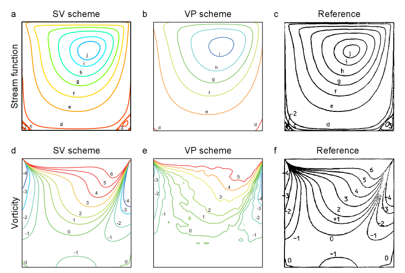
Fig. 1 show the contour plots of the stream function and vorticity obtained from the numerical calculations of cavity flow at $Re=100$, in the following order: SV scheme, VP scheme, and Ghia et al.’s high-order finite difference method. Tables 1 and 2 present the contour values used in these plots (the same values are used for the contour plots in Fig. 2 and subsequent ones). For $Re=100$, it can be said that both SV scheme and VP scheme yield the same trends in the stream function and vorticity as those obtained by Ghia et al. However, from Fig. 1a and b, it is clear that secondary vortices at the bottom corners are well reproduced in the SV scheme, whereas they are hardly reproduced in the VP scheme.

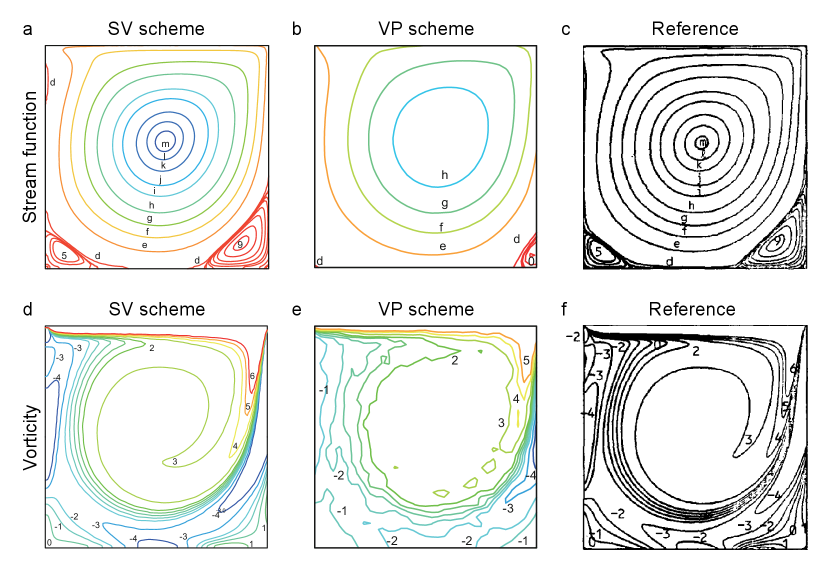
Similarly, Fig. 2 presents the contour plots of the stream function and vorticity obtained from the numerical experiments for $Re=1,000$, and Fig. 3 show the results for $Re=10,000$, in the order of SV scheme, VP scheme, and Ghia et al.’s high-order finite difference method. From Ghia et al.’s numerical results, it can be observed that at $Re=1,000$ (Fig. 2c), secondary vortices form in the corners of the bottom surface, and at $Re=10,000$ (Fig. 3c), secondary and tertiary vortices form in the corners of the bottom surface, and secondary vortices form near one of the corners of the ceiling. This reproduction can also be confirmed in SV scheme (Fig. 2a, Fig. 3a). On the other hand, in VP scheme Fig. 2b, Fig. 3b), the small vortices are hardly reproduced. Additionally, the contour values of vorticity in SV scheme (Fig. 2e, Fig. 3e) and Ghia et al.’s high-order finite difference method (Fig. 2f, Fig. 3f) are generally consistent.

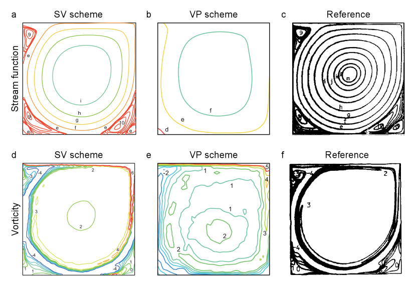
However, in the numerical experiment results of SV scheme for $Re=10,000$ (Fig. 3a, d), discrepancies with Ghia et al.’s numerical results (Fig. 3 c, f) can be seen near the center of the domain. This discrepancy is due to the fact that the velocity magnitude near the center of the domain is relatively underestimated, indicating insufficient analysis accuracy. However, since Ghia and Erturk et al. increased the grid spacing by a factor of two for the high-order finite difference method at $Re=10,000$, it is considered that the insufficient number of particles is the cause in the case of the SPH method.

References

- [1] UKNG Ghia, Kirti N Ghia, and CT Shin. High-Re solutions for incompressible flow using the Navier-Stokes equations and a multigrid method. Journal of computational physics, 48(3):387–411, 1982.
- [2] Ercan Erturk, Thomas C Corke, and Cihan Gökçöl. Numerical solutions of 2-d steady incompressible driven cavity flow at high Reynolds numbers. International Journal for Numerical Methods in Fluids, 48(7):747–774, 2005.
- [3] Leon B Lucy. A numerical approach to the testing of the fission hypothesis. The astronomical journal, 82:1013–1024, 1977.
- [4] Robert A Gingold and Joseph J Monaghan. Smoothed particle hydrodynamics-theory and application to non-spherical stars. Monthly notices of the royal astronomical society, 181:375–389, 1977.
- [5] Gui-Rong Liu and MB Liu. Smoothed particle hydrodynamics: a meshfree particle method. World Scientific, 2003.
- [6] Rui Xu, Peter Stansby, and Dominique Laurence. Accuracy and stability in incompressible SPH (ISPH) based on the projection method and a new approach. Journal of Computational Physics, 228(18):6703–6725, 2009.