Number Theoretic Accelerated Learning of Physics-Informed Neural Networks
Abstract
Physics-informed neural networks solve partial differential equations by training neural networks. Since this method approximates infinite-dimensional PDE solutions with finite collocation points, minimizing discretization errors by selecting suitable points is essential for accelerating the learning process. Inspired by number theoretic methods for numerical analysis, we introduce good lattice training and periodization tricks, which ensure the conditions required by the theory. Our experiments demonstrate that GLT requires 2–7 times fewer collocation points, resulting in lower computational cost, while achieving competitive performance compared to typical sampling methods.
Introduction
Many real-world phenomena can be modeled as partial differential equations (PDEs), and solving PDEs has been a central topic in computational science. The applications include, but are not limited to, weather forecasting, vehicle design (Hirsch2006), economic analysis (Achdou2014), and computer vision (Logan2015). A PDE is expressed as , where is a (possibly nonlinear) differential operator, and is an unknown function on the domain . For most PDEs that appear in physical simulations, the well-posedness (the uniqueness of the solution and the continuous dependence on the initial and boundary conditions) has been well-studied and is typically guaranteed under certain conditions. To solve PDEs, various computational techniques have been explored, including finite difference methods, finite volume methods, and spectral methods (Furihata2010; Morton2005; Thomas1995). However, the development of computer architecture has become slower, leading to a growing need for computationally efficient alternatives. A promising approach is physics-informed neural networks (PINNs) (Raissi2019), which train a neural network by minimizing the physics-informed loss (Wang2022b; Wang2023). This is typically the squared error of the neural network’s output from the PDE averaged over a finite set of collocation points , , encouraging the output to satisfy the equation .
| |
|
|
| uniformly random | uniformly spaced | LHS |
| |
|
|
| Sobol sequence | proposed GLT | proposed GLT (folded) |
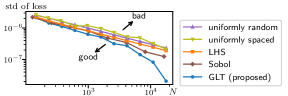
However, the solutions to PDEs are inherently infinite-dimensional, and any distance involving the output or the solution needs to be defined by an integral over the domain . In this regard, the physics-informed loss serves as a finite approximation to the squared 2-norm on the function space for , and hence the discretization errors should affect the training efficiency. A smaller number of collocation points leads to a less accurate approximation and inferior performance, while a larger number increases the computational cost (Bihlo2022; Sharma2022). Despite the importance of selecting appropriate collocation points, insufficient emphasis has been placed on this aspect. Raissi2019, Zeng2023, and many other studies employed Latin hypercube sampling (LHS) to determine the collocation points. Alternative approaches include uniformly random sampling (i.e., the Monte Carlo method) (Jin2021; Krishnapriyan2022) and uniformly spaced sampling (Wang2021c; Wang2022a). These methods are exemplified in Fig. 1.
In the field of numerical analysis, the relationship between integral approximation and collocation points has been extensively investigated. Accordingly, some studies have used quasi-Monte Carlo methods, specifically the Sobol sequence, which approximate integrals more accurately than the Monte Carlo method (Lye2020; Longo2021; Mishra2021). For further improvement, this paper proposes good lattice training (GLT) for PINNs and their variants, such as the competitive PINN (CPINN) (Zeng2023) and physics-informed neural operator (Li2021e; Rosofsky2023). The GLT is inspired by number theoretic methods for numerical analysis, providing an optimal set of collocation points depending on the initial and boundary conditions, as shown in Fig. 1. Our experiments demonstrate that the proposed GLT requires far fewer collocation points than comparison methods while achieving similar errors, significantly reducing computational cost. The contribution and significance of the proposed GLT are threefold.
Computationally Efficient: The proposed GLT offers an optimal set of collocation points to compute a loss function that can be regarded as a finite approximation to an integral over the domain, such as the physics-informed loss, if the activation functions of the neural networks are smooth enough. It requires significantly fewer collocation points to achieve accuracy of solutions and system identifications comparable to other methods, or can achieve lower errors with the same computational budget.
Applicable to PINNs Variants: As the proposed GLT changes only the collocation points, it can be applied to various variants of PINNs without modifying the learning algorithm or objective function. In this study, we investigate a specific variant, the CPINNs (Zeng2023), and demonstrate that CPINNs using the proposed GLT achieve superior convergence speed with significantly fewer collocation points than CPINNs using LHS.
Theoretically Solid: Number theory provides a theoretical basis for the efficacy of the proposed GLT. Existing methods based on quasi-Monte Carlo methods are inferior to the proposed GLT in theoretical performance, or at least require the prior knowledge about the smoothness of the solution and careful adjustments of hyperparameters (Longo2021). On the other hand, the proposed GLT is free from these prior knowledge or adjustments and achieves better performances depending on the smoothness and the neural network, which is a significant advantage.
Related Work
Neural networks are a powerful tool for processing information and have achieved significant success in various fields (He2015a; Vaswani2017), including black-box system identification, that is, to learn the dynamics of physical phenomena from data and predict their future behaviors (Chen2018e; Chen1990; Wang1998). By integrating knowledge from analytical mechanics, neural networks can learn dynamics that adheres to physical laws and even uncover these laws from data (Finzi2020; Greydanus2019; Matsubara2023ICLR).
Neural networks have also gained attention as computational tools for solving differential equations, particularly PDEs (Dissanayake1994; Lagaris1998). Recently, Raissi2019 introduced an elegant refinement to this approach and named it PINNs. The key concept behind PINNs is the physics-informed loss (Wang2022b; Wang2023). This loss function evaluates the extent to which the output of the neural network satisfies a given PDE and its associated initial and boundary conditions . The physics-informed loss can be integrated into other models like DeepONet (Lu2021a; Wang2023) or used for white-box system identifications (that is, adjusting the parameters of known PDEs so that their solutions fit observations).
PINNs are applied to various PDEs (Bihlo2022; Jin2021; Mao2020), with significant efforts in improving learning algorithms and objective functions (Hao2023; Heldmann2023; Lu2022; Pokkunuru2023; Sharma2022; Zeng2023). Objective functions are generally based on PDEs evaluated at a finite set of collocation points rather than data. Bihlo2022; Sharma2022 have shown a trade-off between the number of collocation points (and hence computational cost) and the accuracy of the solution. Thus, selecting collocation points that efficiently cover the entire domain is essential for achieving better results. Some studies have employed quasi-Monte Carlo methods, specifically the Sobol sequence, to determine the collocation points (Lye2020; Mishra2021), but their effectiveness depends on knowledge of the solution’s smoothness and hyperparameter adjustments (Longo2021).
Method
Theoretical Error Estimate of PINNs
For simplicity, we consider PDEs defined on an -dimensional unit cube . PINNs employ a PDE that describes the target physical phenomena as loss functions. Specifically, first, an appropriate set of collocation points is determined, and then the sum of the residuals of the PDE at these points
| (1) |
is minimized as a loss function, where is a differential operator. The physics-informed loss satisfies . Then, the neural network’s output becomes an approximate solution of the PDE. However, for to be the exact solution, the loss function should be 0 for all , not just at collocation points. Therefore, the following integral must be minimized as the loss function:
| (2) |
In other words, the practical minimization of (1) essentially minimizes the approximation of (2) with the expectation that (2) will be small enough, and hence becomes an accurate approximation to the exact solution.
More precisely, we show the following theorem, which is an improvement of an existing error analysis (Mishra2023estimates) in the sense that the approximation error bound of neural networks is considered.
Theorem 1.
Suppose that the class of neural networks used for PINNs includes an -approximator to the exact solution to the PDE : , and that (1) is an -approximation of for the approximated solution and also for : for and . Suppose also that there exist and such that Then,
For a proof, see Appendix “Theoretical Background.” is determined by the architecture of the network and the function space to which the solution belongs. For example, approximation rates of neural networks in Sobolev spaces are given in GUHRING2021107. This explains why increasing the number of collocation points beyond a certain point does not further reduce the error. depends on the accuracy of the approximation of the integral. In this paper, we investigate a training method that easily gives small .
One standard strategy often used in practice is to set ’s to be uniformly distributed random numbers, which can be interpreted as the Monte Carlo approximation of the integral (2). As is widely known, the Monte Carlo method can approximate the integral within an error of independently from the number of dimensions (Sloan1994-cl). However, most PDEs for physical simulations are two to four-dimensional, incorporating a three-dimensional space and a one-dimensional time. Hence, in this paper, we propose a sampling strategy specialized for low-dimensional cases, inspired by number-theoretic numerical analysis.
Good Lattice Training
In this section, we propose the good lattice training (GLT), in which a number theoretic numerical analysis is used to accelerate the training of PINNs (Niederreiter1992-qb; Sloan1994-cl; Zaremba1972-gj). In the following, we use some tools from this theory.
While our target is a PDE on the unit cube , we now treat the loss function as periodic on with a period of 1. Then, we define a lattice.
Definition 2 (Sloan1994-cl).
A lattice in is defined as a finite set of points in that is closed under addition and subtraction.
Given a lattice , the set of collocation points is defined as . Considering that the loss function to be minimized is (2), it is desirable to determine the lattice (and hence the set of collocation points ’s) so that the difference of the two functions is minimized.
Suppose that is smooth enough, admitting the Fourier series expansion:
where denotes the imaginary unit and . Substituting this into (1) yields
| (3) |
because the Fourier mode of is equal to the integral . Before optimizing (3), the dual lattice of lattice and an insightful lemma are introduced as follows.
Definition 3 (Zaremba1972-gj).
A dual lattice of a lattice is defined as .
Lemma 4 (Zaremba1972-gj).
For , it holds that
Lemma 4 follows directly from the properties of Fourier series. Based on this lemma, we restrict the lattice point to the form with a fixed integer vector ; the set of collocation points is . Then, instead of searching ’s, a vector is searched. By restricting to this form, ’s can be obtained automatically from a given , and hence the optimal collocation points ’s do not need to be stored as a table of numbers, making a significant advantage in implementation. Another advantage is theoretical; the optimization problem of the collocation points can be reformulated in a number theoretic way. In fact, for as shown above, it is confirmed that . If then there exists an such that and hence . Conversely, if , clearly .
From the above lemma,
| (4) |
and hence the collocation points ’s should be determined so that (4) becomes small. This problem is a number theoretic problem in the sense that it is a minimization problem of finding an integer vector subject to the condition . This problem has been considered in the field of number theoretic numerical analysis. In particular, optimal solutions have been investigated for integrands in the Korobov spaces, which are spaces of functions that satisfy a certain smoothness condition.
Definition 5 (Zaremba1972-gj).
The function space that is defined as is called the Korobov space, where is the Fourier coefficients of and for .
It is known that if is an integer, for a function to be in , it is sufficient that has continuous partial derivatives . For example, if a function has continuous , then . Hence, if and the neural network belong to Koborov space,
| (5) |
Here, we introduce a theorem in the field of number theoretic numerical analysis:
Theorem 6 (Sloan1994-cl).
For integers and , there exists a such that
for .
The main result of this paper is the following.
Theorem 7.
Suppose that the activation function of and hence itself are sufficiently smooth so that there exists an such that . Then, for given integers and , there exists an integer vector such that is a “good lattice” in the sense that
| (6) |
Intuitively, if satisfies certain conditions, we can find a set of collocation points with which the objective function (1) approximates the integral (2) only within an error of . This rate is much better than that of the uniformly random sampling (i.e., the Monte Carlo method), which is of (Sloan1994-cl), if the activation function of and hence the neural network itself are sufficiently smooth so that for a large . Hence, in this paper, we call the training method that minimizes (1) for a lattice satisfying (6) the good lattice training (GLT).
While any set of collocation points that satisfies the above condition will have the same convergence rate, a set constructed by the vector that minimizes (5) leads to better accuracy. When , it is known that a good lattice can be constructed by setting and , where denotes the -th Fibonacci number (Niederreiter1992-qb; Sloan1994-cl). In general, an algorithm exists that can determine the optimal with a computational cost of . See Appendix “Theoretical Background” for more details. Also, we can retrieve the optimal from numerical tables found in references, such as Fang1994; Keng1981.
Periodization and Randomization Tricks
The integrand of the loss function (2) does not always belong to the Korobov space with high smoothness . To align the proposed GLT with theoretical expectations, we propose periodization tricks for ensuring periodicity and smoothness.
Given an initial condition at time , the periodicity is ensured by extending the lattice twice as much along the time coordinate and folding it. Specifically, instead of , we use as the time coordinate that satisfies if and otherwise (see the lower right panel of Fig. 1, where the time is put on the horizontal axis). Also, while not mandatory, we combine the initial condition and the neural network’s output as , thereby ensuring the initial condition, where denotes the set of coordinates except for the time coordinate . A similar idea was proposed in Lagaris1998, which however does not ensure the initial condition strictly. If a periodic boundary condition is given to the -th space coordinate, we bypass learning it and instead map the coordinate to a unit circle in two-dimensional space. Specifically, we map to , assuring the loss function to take the same value at the both edges ( and ) and be periodic. Given a Dirichlet boundary condition at to the -th axis, we multiply the neural network’s output by , and treat the result as the approximated solution. This ensures the Dirichlet boundary condition is met, and the loss function takes zero at the boundary , thereby ensuring the periodicity. If a more complicated Dirichlet boundary condition is given, one can fold the lattice along the space coordinate in the same manner as the time coordinate and ensure the periodicity of the loss function .
These periodization tricks aim to satisfy the periodicity conditions necessary for GLT to exhibit the performance shown in Theorem 7. However, they are also available for other sampling methods and potentially improve the practical performance by liberating them from the effort of learning initial and boundary conditions.
Since the GLT is grounded on the Fourier series foundation, it allows for the periodic shifting of the lattice. Hence, we randomize the collocation points as
where follows the uniform distribution over the unit cube . Our preliminary experiments confirmed that, if using the stochastic gradient descent (SGD) algorithm, resampling the random numbers at each training iteration prevents the neural network from overfitting and improves training efficiency. We call this approach the randomization trick.
Limitations
Not only is this true for the proposed GLT, but most strategies to determine collocation points are not directly applicable to non-rectangular or non-flat domain (Shankar2018). To achieve the best performance, the PDEs should be transformed to such a domain by an appropriate coordinate transformation. See Knupp2020-ix; Thompson1985-tx for examples.
Previous studies on numerical analysis addressed the periodicity and smoothness conditions on the integrand by variable transformations (Sloan1994-cl) (see also Appendix “Theoretical Background”). However, our preliminary experiments confirmed that it did not perform optimally in typical problem settings. Intuitively, these variable transformations reduce the weights of regions that are difficult to integrate, suppressing the discretization error. This implies that, when used for training, the regions with small weights remain unlearned. As a viable alternative, we introduced the periodization tricks to ensure periodicity.
The performance depends on the smoothness of the physics-informed loss, and hence on the smoothness of the neural network and the true solution. See Appendix “Theoretical Background” for details.
Experiments and Results
Physics-Informed Neural Networks
We modified the code from the official repository111https://github.com/maziarraissi/PINNs (MIT license) of Raissi2019, the original paper on PINNs. We obtained the datasets of the nonlinear Schrödinger (NLS) equation, Korteweg–De Vries (KdV) equation, and Allen-Cahn (AC) equation from the repository. The NLS equation governs wave functions in quantum mechanics, while the KdV equation models shallow water waves, and the AC equation characterizes phase separation in co-polymer melts. These datasets provide numerical solutions to initial value problems with periodic boundary conditions. Although they contain numerical errors, we treated them as the true solutions . These equations are nonlinear versions of hyperbolic or parabolic PDEs. Additionally, as a nonlinear version of an elliptic PDE, we created a dataset for -dimensional Poisson’s equation, which produces analytically solvable solutions with modes with the Dirichlet boundary condition. We examined the cases where . See Appendix “Experimental Settings” for further information.
Unless otherwise stated, we followed the repository’s experimental settings for the NLS equation. The physics-informed loss was defined as given collocation points . This can be regarded as a finite approximation to the squared 2-norm . The state of the NLS equation is complex; we simply treated it as a 2D real vector for training and used its absolute value for evaluation and visualization. Following Raissi2019, we evaluated the performance using the relative error, which is the normalized squared error at predefined collocation points . This is also a finite approximation to .
We applied the above periodization tricks to each test and model for a fair comparison. For Poisson’s equation with , which gives the exact solutions, we followed the original learning strategy using the L-BFGS-B method preceded by the Adam optimizer (Kingma2014b) for 50,000 iterations to ensure precise convergence. For other datasets, which contain the numerical solutions, we trained PINNs using the Adam optimizer with cosine decay of a single cycle to zero (Loshchilov2017) for 200,000 iterations and sampled a different set of collocation points at each iteration. See Appendix “Experimental Settings” for details.
We determined the collocation points using uniformly random sampling, uniformly spaced sampling, LHS, the Sobol sequence, and the proposed GLT. For the GLT, we took the number of collocation points and the corresponding integer vector from numerical tables in (Fang1994; Keng1981). We used the same values for uniformly random sampling and LHS to maintain consistency. For uniformly spaced sampling, we selected numbers for that were closest to a number used in the GLT, creating a unit cube of points on each side. We additionally applied the randomization trick. For the Sobol sequence, we used for due to its theoretical background. We conducted five trials for each number and each method. All experiments were conducted using Python v3.7.16 and tensorflow v1.15.5 (tensorflow) on servers with Intel Xeon Platinum 8368.
| # of points | relative error | ||||||||||
| NLS | KdV | AC | Poisson | NLS | KdV | AC | Poisson | ||||
|
|
uniformly random | 4,181 | 4,181 | 4,181 | 4,181 | 1,019 | 3.11 | 2.97 | 1.55 | 28.53 | 0.28 |
|
|
|||||||||||