Null hypersurfaces as wave fronts in Lorentz-Minkowski space

S. Akamine, A. Honda, M. Umehara and K. Yamada Department of Liberal Arts, College of Bioresource Sciences, Nihon University,1866 Kameino, Fujisawa, Kanagawa, 252-0880, Japan [email protected] Department of Applied Mathematics, Faculty of Engineering, Yokohama National University, 79-5 Tokiwadai, Hodogaya, Yokohama 240-8501, Japan [email protected] Department of Mathematical and Computing Sciences, Tokyo Institute of Technology, Tokyo 152-8552, Japan [email protected] Department of Mathematics, Tokyo Institute of Technology, Tokyo 152-8551, Japan [email protected]

(Date: June 10, 2024)

Abstract.

In this paper, we show that “ $L$ -complete null hypersurfaces” (i.e. ruled hypersurfaces foliated by entirety of light-like lines) as wave fronts in the $(n+1)$ -dimensional Lorentz-Minkowski space are canonically induced by hypersurfaces in the $n$ -dimensional Euclidean space. As an application, we show that most of null wave fronts can be realized as restrictions of certain $L$ -complete null wave fronts. Moreover, we determine $L$ -complete null wave fronts whose singular sets are compact.

Key words and phrases:

light-like hypersurface, null hypersurface, singular point, wave front

2010 Mathematics Subject Classification:

Primary 53C50; Secondary 53C42, 53B30.

The first author was partially supported by the Grant-in-Aid for Young Scientists No. 19K14527. The second author was partially supported by the Grant-in-Aid for Young Scientists No. 19K14526 and (B) No. 20H01801. The third and fourth authors were partially supported by (B) No. 21H00981 and (B) No. 17H02839, respectively, from Japan Society for the Promotion of Science.

Introduction

We denote by ${\mathbb{R}}^{n+1}_{1}$ the $(n+1)$ -dimensional Lorentz-Minkowski space. A null hypersurface in ${\mathbb{R}}^{n+1}_{1}$ is a $C^{\infty}$ -immersion whose induced metric degenerates everywhere. Such a hypersurface is also called a light-like hypersurface and is locally foliated by light-like lines (cf. [2, Fact 2.6]). Roughly speaking, a null hypersurface is said to be $L$ -complete if each light-like line is the entirety of a straight line in ${\mathbb{R}}^{n+1}_{1}$ (see Definition 2.1 for details).

In the authors’ previous work [2], it was shown that $L$ -complete null immersed hypersurfaces in ${\mathbb{R}}^{n+1}_{1}$ are totally geodesic. As is clear from this previous work, the study of global properties of such surfaces, considering only immersions is too restrictive. In this paper, we shall investigate the global behavior of null hypersurfaces with singular points in ${\mathbb{R}}^{n+1}_{1}$ .

More precisely, instead of immersions, we shall introduce null hypersurfaces as wave fronts (see Section 1). It can be easily observed that each hypersurface in the $n$ -dimensional Euclidean space ${\mathbb{R}}^{n}_{0}$ ( $n\geq 2$ ) induces an associated parallel family, and this family can be considered as a section of a null hypersurface in ${\mathbb{R}}^{n+1}_{1}$ . For example, the light-cone

(0.1)

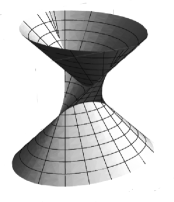
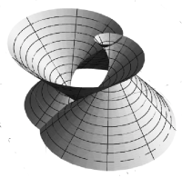
\Lambda^{n}:=\Big{\{}(t,x_{1},\ldots,x_{n})\in{\mathbb{R}}^{n+1}_{1}\,;\,(x_{1})^{2}+\cdots+(x_{n})^{2}=t^{2}\Big{\}}

is a typical example of an $L$ -complete null wave front, which corresponds to the family of parallel hypersurfaces of the unit sphere $S^{n-1}$ in ${\mathbb{R}}^{n}_{0}$ centered at the origin. The origin as the cone-like singular point of $\Lambda^{n}$ corresponds to the parallel hypersurface of $S^{n-1}$ just shrinking to a point. In general, a null hypersurface may have various singular points. For example, for each $a\in(0,1]$ , we consider an ellipse

(0.2)

\gamma(\theta):=(a\cos\theta,\,\sin\theta)\qquad(0\leq\theta\leq 2\pi),

in the Euclidean plane. Let ${\mathbf{n}}(\theta)$ be the leftward unit normal vector field along $\gamma$ . Then the map $F_{a}:{\mathbb{R}}\times({\mathbb{R}}/2\pi{\mathbb{Z}})\to{\mathbb{R}}^{3}_{1}$ defined by

(0.3)

F_{a}(t,\theta):=(0,\gamma(\theta))+t(1,{\mathbf{n}}(\theta))\qquad(a\in(0,1])

gives a null wave front having cuspidal edges and four swallowtails whenever $0<a<1$ (the definitions of cuspidal edges and swallowtails are given in [3]). Each slice of the image of $F_{a}$ by the horizontal plane $t=t_{0}$ corresponds to the parallel curve of the ellipse $\gamma$ of equi-distance $t_{0}$ . When $a=1$ , the image of $F_{1}$ just coincides with the light-cone $\Lambda^{2}$ of ${\mathbb{R}}^{3}_{1}$ .

Refer to caption — Figure 1. The complete null wave front associated with the family of parallel curves of the ellipse of $a=1/2$ .

In Section 2, we prove the converse assertion (cf. Theorem 2.6) as a fundamental theorem of null wave fronts, which states that any $L$ -complete null wave fronts in ${\mathbb{R}}^{n+1}_{1}$ are induced from wave fronts in ${\mathbb{R}}^{n}_{0}$ . As a consequence, we can say that an $L$ -complete null wave front is associated with the parallel family of a wave front in ${\mathbb{R}}^{n}_{0}$ .

We give two applications of this fundamental theorem. In Section 3, we show a “structure theorem of null hypersurfaces” (cf. Theorem 3.4) which asserts that most of null wave fronts (for example, real analytic null wave fronts and $C^{\infty}$ null wave fronts with a certain genericity) can be obtained as restrictions of $L$ -complete null wave fronts. There are several interesting geometric structures on null hypersurfaces in ${\mathbb{R}}^{n+1}_{1}$ without assuming $L$ -completeness (cf. [4, 7]). The authors hope that this theorem might play an important role in the further study of null hypersurfaces.

On the other hand, an $L$ -complete null wave front in ${\mathbb{R}}^{n+1}_{1}$ is called complete if its singular set is a non-empty compact subset in the domain of definition. For example, the light-cone $\Lambda^{n}$ in ${\mathbb{R}}^{n+1}_{1}$ and the null wave front $F_{a}$ in ${\mathbb{R}}^{3}_{1}$ given in (0.3) are complete. In Section 4, as the deepest application of the fundamental theorem, we show that each of complete null wave fronts corresponds to a parallel family of a closed convex hypersurface in ${\mathbb{R}}^{n}_{0}$ if $n\geq 3$ (cf. Theorem 4.4). When $n=2$ , we show that complete null wave fronts are induced by parallel families of locally convex closed regular curves in the Euclidean plane ${\mathbb{R}}^{2}_{0}$ . If the curve is an ellipse, the null wave front corresponds to $F_{a}$ as above (see Figure 1).

It should be remarked that the classical four vertex theorem for closed convex curves implies the existence of four non-cuspidal edge singular points on complete null wave fronts with embedded ends in ${\mathbb{R}}^{3}_{1}$ (cf. Corollary 4.6).

There is one point to note when reading this paper: Readers who are interested only in the fundamental theorem for $L$ -complete null wave fronts or complete null wave fronts can skip Section 3. In fact, Section 4 is devoted to properties of complete null wave fronts and does not refer to Section 3. Appendix A of this paper is required for Section 2, but Appendix B is used for Section 3, so such readers also do not need to read Appendix B.

1. Properties of null wave fronts in ${\mathbb{R}}^{n+1}_{1}$

We first recall the definition of wave fronts. Let $({\mathbb{R}}^{n+1})^{*}$ be the dual vector space of ${\mathbb{R}}^{n+1}$ , and we denote by $P^{*}({\mathbb{R}}^{n+1})$ the projective space associated with $({\mathbb{R}}^{n+1})^{*}$ . We let

\pi:({\mathbb{R}}^{n+1})^{*}\setminus\{{\mathbf{0}}\}\to P^{*}({\mathbb{R}}^{n+1})

be the canonical projection. Then, for each element $\zeta\in P^{*}({\mathbb{R}}^{n+1})$ , there exists a linear function $\omega:{\mathbb{R}}^{n+1}\to{\mathbb{R}}$ (which is an element of $({\mathbb{R}}^{n+1})^{*}\setminus\{{\mathbf{0}}\}$ ) such that $\pi(\omega)=\zeta$ . Since the kernel of $\omega$ is invariant under non-zero scalar multiplications, the $n$ -dimensional subspace

\operatorname{Ker}(\zeta):=\operatorname{Ker}(\omega)

is well-defined.

In this paper, we set $r=\infty$ or $r=\omega$ and “ $C^{r}$ ” means smoothness if $r=\infty$ and real analyticity if $r=\omega$ . We fix a $C^{r}$ -differentiable $n$ -manifold $M^{n}$ .

Definition 1.1.

Let $F:M^{n}\to{\mathbb{R}}^{n+1}$ be a $C^{r}$ -map. Then the map $F$ is called a $C^{r}$ -wave front (or simply a $C^{r}$ -front) if for each $p\in M^{n}$ , there exist a neighborhood $U$ of $p$ and a $C^{r}$ -map $\tilde{\alpha}:U\to({\mathbb{R}}^{n+1})^{*}\setminus\{{\mathbf{0}}\}$ such that

(1)

$\alpha:=\pi\circ\tilde{\alpha}$ satisfies $(dF)_{q}({\mathbf{v}})\in\operatorname{Ker}(\alpha_{q})\,\,(q\in U,\,\,{\mathbf{v}}\in T_{q}M^{n})$ , and
(2)

$L:=(F,\alpha):U\to{\mathbb{R}}^{n+1}\times P^{*}({\mathbb{R}}^{n+1})$ is an immersion.

Moreover, if we can take $U=M^{n}$ , the map $F$ is said to be co-orientable. In this case, $\alpha:M^{n}\to P^{*}({\mathbb{R}}^{n+1})$ is called the Gauss map of $F$ , and the map $\tilde{\alpha}:M^{n}\to({\mathbb{R}}^{n+1})^{*}\setminus\{{\mathbf{0}}\}$ is called the lift of $\alpha$ .

If a $C^{r}$ -wave front $F$ is not co-orientable, taking the double covering $\hat{\pi}:\hat{M}^{n}\to M^{n}$ , the composition $F\circ\hat{\pi}$ becomes a co-orientable wave front. So without loss of generality, we may assume that $F$ itself is co-orientable.

We let ${\mathbb{R}}^{n+1}_{1}$ be Lorentz-Minkowski $(n+1)$ -space of signature $(-+\cdots+)$ , and denote by $\left\langle{\,},{\,}\right\rangle$ the canonical Lorentzian inner product on ${\mathbb{R}}^{n+1}_{1}$ .

Proposition 1.2.

Let $F:M^{n}\to{\mathbb{R}}^{n+1}_{1}$ be a $($ co-orientable $)$ $C^{r}$ -wave front. Then there exists a vector field $\hat{\xi}$ without zeros $($ which can be considered as a map $\hat{\xi}:M^{n}\to{\mathbb{R}}^{n+1}_{1}\setminus\{{\mathbf{0}}\})$ such that

\left\langle{\hat{\xi}_{p}},{dF({\mathbf{v}})}\right\rangle=0\qquad(p\in M^{n},\,\,{\mathbf{v}}\in T_{p}M^{n}).

A vector field $\hat{\xi}$ along $F$ given in Proposition 1.2 is called a normal vector field along $F$ .

Proof.

Let $\tilde{\alpha}$ be a lift of the Gauss map of $F$ . Since $\left\langle{\,},{\,}\right\rangle$ is non-degenerate, there exists a vector field $\hat{\xi}$ on $M^{n}$ along $F$ such that

(1.1)

\left\langle{\hat{\xi}_{p}},{{\mathbf{x}}}\right\rangle=\tilde{\alpha}_{p}({\mathbf{x}})\qquad({\mathbf{x}}\in T_{F(p)}{\mathbb{R}}^{n+1}_{1}).

Since $\alpha_{p}\neq{\mathbf{0}}$ for each $p$ , the vector field $\hat{\xi}$ has no zeros on $M^{n}$ . ∎

We then introduce ‘null wave fronts’ as follows:

Definition 1.3.

In the setting of Proposition 1.2, the $C^{r}$ -wave front $F:M^{n}\to{\mathbb{R}}^{n+1}_{1}$ is said to be null or light-like if $\hat{\xi}_{p}$ points in the light-like direction in ${\mathbb{R}}^{n+1}_{1}$ at each $p\in M^{n}$ .

We denote by $(\,,\,)_{E}$ the canonical positive definite inner product on ${\mathbb{R}}^{n+1}(={\mathbb{R}}^{n+1}_{1})$ .

Definition 1.4 ( $E$ -normalized normal vector field).

Let $F:M^{n}\to{\mathbb{R}}^{n+1}_{1}$ be a (co-orientable) null $C^{r}$ -wave front. A normal vector field $\hat{\xi}$ along $F$ is said to be $E$ -normalized if $\hat{\xi}$ points in the future direction and satisfies $|\hat{\xi}|_{E}=\sqrt{2}$ , where

|{\mathbf{v}}|_{E}:=\sqrt{({\mathbf{v}},{\mathbf{v}})_{E}}\qquad({\mathbf{v}}\in{\mathbb{R}}^{n+1}_{1}).

Since such a vector field $\hat{\xi}$ is uniquely determined, we denote it by $\hat{\xi}_{E}$ .

Remark 1.5.

One can replace $\sqrt{2}$ with any positive constant $c$ . However, the choice of $c:=\sqrt{2}$ makes sense in the following reason: As we will show in Theorem 2.3, a hypersurface $f:\Sigma^{n-1}\to{\mathbb{R}}^{n}_{0}$ in Euclidean space ${\mathbb{R}}^{n}_{0}$ with unit normal vector field $\nu$ induces null wave fronts $F_{\pm}:{\mathbb{R}}\times\Sigma^{n-1}\to{\mathbb{R}}^{n+1}_{1}$ whose $E$ -normalized normal vector fields are given by $\hat{\xi}:=(1,\pm\nu)$ .

We can always take the $E$ -normalized normal vector field for a given co-orientable null wave front $F$ as follows: By Proposition 1.2, we can take a normal vector field $\hat{\xi}$ along $F$ . Since $F$ is light-like, $\hat{\xi}$ gives a light-like vector field along $F$ . By replacing $\hat{\xi}$ by $-\hat{\xi}$ , we may assume that $\hat{\xi}$ points in the future direction, and

\hat{\xi}_{E}:=\frac{\sqrt{2}}{|\hat{\xi}|_{E}}\hat{\xi}

gives the desired vector field.

Lemma 1.6.

Let $F:M^{n}\to{\mathbb{R}}^{n+1}_{1}$ be a $($ co-orientable $)$ null wave front. Then

(1.2)

{\mathcal{L}}_{F}:=(F,\hat{\xi}_{E}):M^{n}\to{\mathbb{R}}^{n+1}_{1}\times{\mathbb{R}}^{n+1}_{1}

is an immersion into ${\mathbb{R}}^{n+1}_{1}\times{\mathbb{R}}^{n+1}_{1}$ .

We call this ${\mathcal{L}}_{F}:M^{n}\to{\mathbb{R}}^{n+1}_{1}\times{\mathbb{R}}^{n+1}_{1}$ the canonical lift of $F$ .

Proof.

We denote by $S^{n}(\sqrt{2})$ the sphere of radius $\sqrt{2}$ centered at the origin in ${\mathbb{R}}^{n+1}_{1}$ with respect to the metric $(\,,\,)_{E}$ . Since

S^{n}(\sqrt{2})\ni{\mathbf{v}}\mapsto\pi(\left\langle{{\mathbf{v}}},{*}\right\rangle)\in P^{*}({\mathbb{R}}^{n+1})

gives the double covering of $P^{*}({\mathbb{R}}^{n+1})$ , it can be easily observed that ${\mathcal{L}}_{F}$ is an immersion into ${\mathbb{R}}^{n+1}_{1}\times S^{n}(\sqrt{2})$ if and only if $(F,\pi\circ\tilde{\alpha}):M^{n}\to{\mathbb{R}}^{n+1}\times P^{*}({\mathbb{R}}^{n+1})$ is an immersion, where $\tilde{\alpha}$ is the map $\tilde{\alpha}:M^{n}\to({\mathbb{R}}^{n+1})^{*}\setminus\{{\mathbf{0}}\}$ induced by $\hat{\xi}$ given in (1.1). ∎

The following assertion gives a characterization of null wave fronts:

Proposition 1.7.

Let $F:M^{n}\to{\mathbb{R}}^{n+1}_{1}$ be a $C^{r}$ -map. Then $F$ is a $($ co-orientable $)$ null wave front if and only if there exists a vector field $\hat{\xi}$ along $F$ defined on $M^{n}$ such that

(1)

$(\hat{\xi},\hat{\xi})_{E}=2$ ,
(2)

$\hat{\xi}$ is pointing in the future light-like direction, and
(3)

$(F,\hat{\xi})$ is an immersion into ${\mathbb{R}}^{n+1}_{1}\times{\mathbb{R}}^{n+1}_{1}$ satisfying $\langle\hat{\xi}_{p},dF_{p}({\mathbf{v}})\rangle=0$ for each ${\mathbf{v}}\in T_{p}M^{n}$ $(p\in M^{n})$ .

Proof.

We have already seen that any null wave front in ${\mathbb{R}}^{n+1}_{1}$ uniquely induces an $E$ -normalized normal vector field $\hat{\xi}_{E}$ . So it is sufficient to show the converse. Suppose that $\hat{\xi}$ is a vector field along $F$ satisfying the above three conditions. We let $\tilde{\alpha}:M^{n}\to({\mathbb{R}}^{n+1})^{*}\setminus\{{\mathbf{0}}\}$ be the map given in (1.1). By (1) and (3), $(F,\pi\circ\tilde{\alpha}):M^{n}\to{\mathbb{R}}^{n+1}\times P^{*}({\mathbb{R}}^{n+1})$ is an immersion by the same reason as in the proof of Lemma 1.6. ∎

Lemma 1.8.

Let $F:M^{n}\to{\mathbb{R}}^{n+1}_{1}$ be a null $C^{r}$ -immersion with a normal vector field $\hat{\xi}$ on $M^{n}$ as in Proposition 1.7. Then for each $p\in M^{n}$ , there exists a unique tangent vector $\xi_{p}\in T_{p}M^{n}$ such that $dF(\xi_{p})=\hat{\xi}_{p}$ . Moreover, the correspondence $p\mapsto\xi_{p}$ is $C^{r}$ -differentiable.

Proof.

Since $dF_{p}(T_{p}M^{n})$ is an $n$ -dimensional vector subspace of $T_{F(p)}{\mathbb{R}}^{n+1}_{1}$ at each $p\in M^{n}$ , it holds that

dF_{p}(T_{p}M^{n})=\Big{\{}\hat{{\mathbf{v}}}\in{\mathbb{R}}^{n+1}_{1}\,;\,\left\langle{\hat{{\mathbf{v}}}},{\hat{\xi}_{p}}\right\rangle=0\Big{\}}.

Since $\hat{\xi}_{p}\in dF_{p}(T_{p}M^{n})$ and $dF_{p}$ is injective, the desired vector $\xi_{p}$ should be

\xi_{p}:=(dF_{p})^{-1}(\hat{\xi}_{p})\qquad(p\in M^{n}).

Since $(dF_{p})^{-1}(\hat{\xi}_{p})$ depends smoothly on $p$ , we obtain the assertion. ∎

Later, we will show that the assertion of Lemma 1.8 is extended for null $C^{r}$ -wave fronts (cf. Theorem 1.14). The next assertion is a weak version of Lemma 1.8 for null wave fronts.

Proposition 1.9.

Let $F:M^{n}\to{\mathbb{R}}^{n+1}_{1}$ be a $($ co-orientable $)$ null $C^{r}$ -wave front and $\hat{\xi}$ a normal vector field along $F$ . Then, for each $p\in M^{n}$ , there exists a tangent vector $\boldsymbol{v}\in T_{p}M^{n}$ such that $(dF)_{p}(\boldsymbol{v})=\hat{\xi}_{p}$ .

Proof.

We may assume that $\hat{\xi}=\hat{\xi}_{E}$ . If $F$ gives an immersion at $p$ , then the assertion follows from Lemma 1.8. So we may assume that $p$ is a singular point $($ i.e. is a point where $F$ is not an immersion $)$ of $F$ . We can take a local coordinate system $(u_{1},\ldots,u_{n})$ of $M^{n}$ centered at $p$ such that the family of vectors

(\partial_{u_{1}})_{p}\,\,,\ldots,\,\,(\partial_{u_{r}})_{p}\qquad(r>0)

spans the kernel of $(dF)_{p}$ , where $\partial_{u_{j}}:=\partial/\partial u_{j}$ ( $j=1,\ldots,n$ ). By setting

F_{u_{i}}:=dF(\partial_{u_{i}})\qquad(i=1,\ldots,n),

the vectors $F_{u_{r+1}}(p)\,\,,\ldots,\,\,F_{u_{n}}(p)$ are linearly independent. We denote by $V$ the subspace of ${\mathbb{R}}^{n+1}_{1}$ spanned by these vectors. We set

(1.3)

\hat{\eta}_{i}:=d\hat{\xi}_{E}(\partial_{u_{i}})\qquad(i=1,\ldots,n).

If we think $F$ and $\hat{\xi}_{E}$ are column vector-valued functions, we can consider the $(2n+2)\times n$ -matrix

(1.4)

M_{0}:={\begin{pmatrix}F_{u_{1}}&\cdots&F_{u_{r}}&F_{u_{r+1}}&\cdots&F_{u_{n}}\\ \hat{\eta}_{1}&\cdots&\hat{\eta}_{r}&\hat{\eta}_{r+1}&\cdots&\hat{\eta}_{n}\end{pmatrix}}

at $p$ as the Jacobi matrix of the map $(F,\hat{\xi}_{E})$ of $M^{n}$ into ${\mathbb{R}}^{n+1}_{1}\times{\mathbb{R}}^{n+1}_{1}$ , which can be computed as

M_{0}={\begin{pmatrix}{\mathbf{0}}&\cdots&{\mathbf{0}}&F_{u_{r+1}}(p)&\cdots&F_{u_{n}}(p)\\ \hat{\eta}_{1}(p)&\cdots&\hat{\eta}_{r}(p)&\hat{\eta}_{r+1}(p)&\cdots&\hat{\eta}_{n}(p)\end{pmatrix}}.

Since $F$ is a wave front, the matrix $M_{0}$ is of rank $n$ and so

\hat{\eta}_{1}(p)\,\,,\ldots,\,\,\hat{\eta}_{r}(p)

are linearly independent at $p$ , which gives a basis of the vector space defined by

(1.5)

W:=\left\{\sum_{i=1}^{r}a_{i}\hat{\eta}_{i}(p)\,;\,a_{1},\ldots,a_{r}\in{\mathbb{R}}\right\}.

Suppose $(\hat{\xi}_{E})_{p}$ does not belong to $V$ . We set $N:={\mathbb{R}}(\hat{\xi}_{E})_{p}$ , that is, it is the 1-dimensional vector space generated by $(\hat{\xi}_{E})_{p}$ . By the following Lemma 1.10, $W\cap N=\{{\mathbf{0}}\}$ holds, and $V$ , $W$ and $N$ satisfy the assumption of Lemma A.3 in Appendix A. So we have $W\cap V=\{{\mathbf{0}}\}$ . Since $W$ is of dimension $r$ and $V$ is of dimension $n-r$ , the direct sum $V+W+N$ coincides with ${\mathbb{R}}^{n+1}_{1}$ . Then $(\hat{\xi}_{E})_{p}$ vanishes because $(\hat{\xi}_{E})_{p}$ is perpendicular to $V,W$ and $N$ , a contradiction. Thus, we can find a vector $\boldsymbol{v}\in T_{p}M^{n}$ such that $(\hat{\xi}_{E})_{p}=dF_{p}(\boldsymbol{v})\in V$ . ∎

Lemma 1.10.

The vector space $W$ given in (1.5) is perpendicular to $dF_{p}(T_{p}M^{n})$ in ${\mathbb{R}}^{n+1}_{1}$ . Moreover, $(\hat{\xi}_{E})_{p}$ does not belong to $W$ .

Proof.

As in the proof of Proposition 1.9, we denote by $V$ the subspace of ${\mathbb{R}}^{n+1}_{1}$ spanned by $F_{u_{r+1}}(p)\,\,,\ldots,\,\,F_{u_{n}}(p)$ . Using the notation (1.3), for each $i\in\{1,\ldots,r\}$ and $j\in\{r+1,\ldots,n\}$ , we have

	$\displaystyle\left\langle{F_{u_{j}}},{\hat{\eta}_{i}}\right\rangle$	$\displaystyle={\left\langle{F_{u_{j}}},{\hat{\xi}_{E}}\right\rangle}_{u_{i}}-\left\langle{F_{u_{j}u_{i}}},{\hat{\xi}_{E}}\right\rangle=-\left\langle{F_{u_{j}u_{i}}},{\hat{\xi}_{E}}\right\rangle$
		$\displaystyle=-\left\langle{F_{u_{i}}},{\hat{\xi}_{E}}\right\rangle_{u_{j}}+\left\langle{F_{u_{i}}},{d\hat{\xi}_{E}(\partial_{u_{j}})}\right\rangle=\left\langle{F_{u_{i}}},{\hat{\eta}_{j}}\right\rangle=0$

at $p$ , where we used the fact $F_{u_{i}}(p)={\mathbf{0}}$ . By this computation, we have that

(1.6)

\left\langle{v},{w}\right\rangle=0\qquad(v\in V,\,\,w\in W),

proving the first assertion.

We prove the second assertion. If $(\hat{\xi}_{E})_{p}\in W$ , then we can write $\hat{\xi}_{E}=\sum_{i=1}^{r}a_{i}(\hat{\xi}_{E})_{u_{i}}$ at $p$ . Then it holds that

2=\Big{(}(\hat{\xi}_{E})_{p},(\hat{\xi}_{E})_{p}\Big{)}_{E}=\sum_{i=1}^{r}a_{i}\Big{(}\big{(}(\hat{\xi}_{E})_{u_{i}}\big{)}_{p},\big{(}\hat{\xi}_{E}\big{)}_{p}\Big{)}_{E}=0,

a contradiction. ∎

We next prepare the following:

Proposition 1.11.

Let $F:M^{n}\to{\mathbb{R}}^{n+1}_{1}$ be a null $C^{r}$ -wave front and $\hat{\xi}_{E}$ its associated $E$ -normalized normal vector field. Suppose that $p\in M^{n}$ is a singular point of $F$ . Then

(1)

for each $\delta\in{\mathbb{R}}$ ,

(1.7) $F_{\delta}:=F+\delta\,\hat{\xi}_{E}$

is a null wave front defined on $M^{n}$ , and
(2)

there exists a positive number $\varepsilon_{0}$ such that $F_{\delta}$ $(0<|\delta|<\varepsilon_{0})$ is an immersion at $p$ .

Remark 1.12.

Later, we will show that the image of $F_{\delta}$ coincides with that of $F$ under a suitable assumption of $F$ (see Corollary 2.8).

Proof.

Since $\hat{\xi}_{E}$ is a light-like vector field, it is a normal vector field of $F_{\delta}$ . We set

M_{\delta}:={\begin{pmatrix}(F_{\delta})_{u_{1}}&\cdots&(F_{\delta})_{u_{r}}&(F_{\delta})_{u_{r+1}}&\cdots&(F_{\delta})_{u_{n}}\\ (\hat{\xi}_{E})_{u_{1}}&\cdots&(\hat{\xi}_{E})_{u_{r}}&(\hat{\xi}_{E})_{u_{r+1}}&\cdots&(\hat{\xi}_{E})_{u_{n}}\end{pmatrix}}

for $\delta\in{\mathbb{R}}$ . Since $M_{\delta}$ ( $\delta\neq 0$ ) is obtained by adding the second row to the first row of $M_{0}$ , the pair $(F_{\delta},\hat{\xi}_{E})$ gives an immersion of $M^{n}$ into ${\mathbb{R}}^{n+1}_{1}\times{\mathbb{R}}^{n+1}_{1}$ if and only if $(F,\hat{\xi}_{E})$ is an immersion. So (1) is proved.

We next prove (2). By Proposition 1.9, there exists a vector $\boldsymbol{v}\in T_{p}M^{n}$ such that $dF_{p}(\boldsymbol{v})=(\hat{\xi}_{E})_{p}$ . We then take a local coordinate system $(u_{1},\ldots,u_{n})$ of $M^{n}$ centered at $p$ such that

(\partial_{u_{1}})_{p}\,\,,\ldots,\,\,(\partial_{u_{r}})_{p}\qquad(r>0)

belong to the kernel of $(dF)_{p}$ and $(\partial_{u_{n}})_{p}=\boldsymbol{v}$ . We let $V$ be the subspace of ${\mathbb{R}}^{n+1}_{1}$ , which is spanned by $F_{u_{r+1}}(p)\,\,,\ldots,\,\,F_{u_{n-1}}(p)$ . We consider the $r$ -dimensional vector space $W$ given by (1.5). By Lemma 1.10, it can be easily checked that the three vector subspaces $V,\,\,W$ and $N:={\mathbb{R}}\hat{\xi}_{E}$ satisfy the assumption of Lemma A.3 in Appendix A. So we have

V\cap W=V\cap N=W\cap N=\{{\mathbf{0}}\}.

In particular, the vectors

(\hat{\xi}_{E})_{u_{1}},\,\,\ldots,(\hat{\xi}_{E})_{u_{r}},\,\,F_{u_{r+1}}\,\,,\ldots,\,\,F_{u_{n}}(=\hat{\xi}_{E})

are linearly independent at $p\in M^{n}$ . We fix a non-zero real number $\delta$ . Then we have

	$\displaystyle m(\delta):=$	$\displaystyle\operatorname{rank}\Big{(}dF_{\delta}(\partial_{u_{1}}),\dots,dF_{\delta}(\partial_{u_{r}}),dF_{\delta}(\partial_{u_{r+1}}),\dots,dF_{\delta}(\partial_{u_{n}})\Big{)}$
		$\displaystyle=\operatorname{rank}\Big{(}\delta d\hat{\xi}_{E}(\partial_{u_{1}}),\dots,\delta d\hat{\xi}_{E}(\partial_{u_{r}}),dF(\partial_{u_{r+1}})+\delta d\hat{\xi}_{E}(\partial_{u_{r+1}}),$
		$\displaystyle\phantom{aaaaaaaaaaaaaaaaaaaaaaaaaaaaaaaaa}\dots,dF(\partial_{u_{n}})+\delta d\hat{\xi}_{E}(\partial_{u_{n}})\Big{)}$
		$\displaystyle=\operatorname{rank}\Big{(}d\hat{\xi}_{E}(\partial_{u_{1}}),\dots,d\hat{\xi}_{E}(\partial_{u_{r}}),dF(\partial_{u_{r+1}})+\delta d\hat{\xi}_{E}(\partial_{u_{r+1}}),$
		$\displaystyle\phantom{aaaaaaaaaaaaaaaaaaaaaaaaaaaaaaaaa}\dots,dF(\partial_{u_{n}})+\delta d\hat{\xi}_{E}(\partial_{u_{n}})\Big{)}.$

If $|\delta|$ is sufficiently small, the right-hand side of the last equality is equal to $n$ at $p$ . So we can conclude that $F_{\delta}$ is an immersion on a sufficiently small neighborhood of $p$ for sufficiently small $|\delta|(>0)$ . ∎

Definition 1.13 ( $E$ -normalized null vector field).

Let $F:M^{n}\to{\mathbb{R}}^{n+1}_{1}$ be a null $C^{r}$ -wave front and $\hat{\xi}_{E}$ its associated $E$ -normalized normal vector field. If there exists a $C^{r}$ -differentiable vector field $\xi_{E}$ defined on $M^{n}$ such that $dF(\xi_{E})=\hat{\xi}_{E}$ , then $\xi_{E}$ is called the $E$ -normalized null vector field with respect to $F$ (in fact, $\xi_{E}$ is uniquely determined as follows).

The following is the deepest result in this section, which asserts the existence of $E$ -normalized null vector field:

Theorem 1.14.

Let $F:M^{n}\to{\mathbb{R}}^{n+1}_{1}$ be a null $C^{r}$ -wave front and $\hat{\xi}_{E}$ its associated $E$ -normalized normal vector field. Then there exists a unique $C^{r}$ -differentiable vector field $\xi_{E}$ defined on $M^{n}$ such that

(1)

$dF(\xi_{E})=\hat{\xi}_{E}$ $($ that is, $\xi_{E}$ is the $E$ -normalized null vector field $)$ , and
(2)

the image of each integral curve of $\xi_{E}$ is a part of a light-like line in ${\mathbb{R}}^{n+1}_{1}$ .

Moreover, $dF(T_{p}M^{n})$ is a light-like vector space in ${\mathbb{R}}^{n+1}_{1}$ .

Proof.

Roughly speaking, the key of the proof is that the image of the null wave front $F$ is foliated by light-like lines as mentioned in the introduction, and we will construct a vector field $\xi_{E}$ defined on $M^{n}$ so that each integral curve of $\xi_{E}$ corresponds to the leaf of the foliation as follows.

We fix a point $p\in M^{n}$ arbitrarily. By Proposition 1.11, for a sufficiently small positive number $\delta$ , there exists a neighborhood $U$ of $p$ such that $F_{\delta}$ is an immersion on $U$ . Hence, by Lemma 1.8, there exists a unique $C^{r}$ -differentiable null vector field $\xi_{E}$ satisfying $dF_{\delta}(\xi_{E})=\hat{\xi}_{E}$ on $U$ . We let $\gamma_{q}(t)$ be the integral curve of $\xi_{E}$ such that $\gamma_{q}(0)=q$ for $q\in U$ . Since $\hat{\xi}_{E}$ is a null vector field along $F_{\delta}$ , [2, Fact 2.6] implies that $F_{\delta}\circ\gamma_{q}$ parametrizes a segment of a light-like line. Thus $F_{\delta}\circ\gamma_{q}(t)$ is a geodesic in ${\mathbb{R}}^{n+1}_{1}$ , and so we have $D_{\xi_{E}}dF_{\delta}(\xi_{E})={\mathbf{0}},$ where $D$ is the Levi-Civita connection of ${\mathbb{R}}^{n+1}_{1}$ . So,

dF(\xi_{E})=dF_{\delta}(\xi_{E})-\delta(d\hat{\xi}_{E})(\xi_{E})=\hat{\xi}_{E}-\delta D_{\xi_{E}}dF_{\delta}(\xi_{E})=\hat{\xi}_{E}

holds at $p$ . Since the light-like vector $(\hat{\xi}_{E})_{q}$ ( $q\in U$ ) lies in $dF_{q}(T_{q}M^{n})$ , the vector space $(dF)_{q}(T_{q}M^{n})$ is light-like. Since $p$ is arbitrary, the uniqueness of $\xi_{E}$ implies it can be defined on $M^{n}$ , proving the assertion. ∎

2. A fundamental theorem for $L$ -complete null wave fronts

We first define the following “ $L$ -completeness” of null wave fronts in ${\mathbb{R}}^{n+1}_{1}$ , which is analogous to the case of null immersions given in [2, Definition 2.7].

Definition 2.1.

Let $F:M^{n}\to{\mathbb{R}}^{n+1}_{1}$ be a (co-orientable) null $C^{r}$ -wave front. The map $F$ is called $L$ -complete if for each $p\in M^{n}$ , there exists an integral curve $\gamma:{\mathbb{R}}\to M^{n}$ of the $E$ -normalized null vector field $\xi_{E}$ passing through $p$ such that $F\circ\gamma({\mathbb{R}})$ coincides with an entire light-like line in ${\mathbb{R}}^{n+1}_{1}$ .

The following assertion holds:

Proposition 2.2.

Let $F:M^{n}\to{\mathbb{R}}^{n+1}_{1}$ be a $($ co-orientable $)$ null $C^{r}$ -wave front. Then $F$ is $L$ -complete if and only if its $E$ -normalized null vector field $\xi_{E}$ is complete on $M^{n}$ $($ that is, each integral curve of $\xi_{E}$ is defined on ${\mathbb{R}})$ .

Proof.

Let $\gamma(t)$ be any integral curve of $\xi_{E}$ . Since $|dF(\xi_{E})|_{E}=\sqrt{2}$ , $\gamma(t)$ is parametrized by an affine parametrization of a light-like line. So $\gamma$ is defined on ${\mathbb{R}}$ if and only if the image of $F\circ\gamma$ coincides with the entirety of a line. ∎

We consider the height function

(2.1)

\hat{\tau}:{\mathbb{R}}^{n+1}_{1}\ni{\mathbf{v}}\mapsto-\left\langle{{\mathbf{v}}},{{\mathbf{e}}_{0}}\right\rangle\in{\mathbb{R}}

with respect to the time axis, where ${\mathbf{e}}_{0}:=(1,0,\ldots,0)$ . The level set $\hat{\tau}^{-1}(0)$ is a space-like hyperplane which is isometric to the Euclidean $n$ -space ${\mathbb{R}}^{n}_{0}$ . So, we frequently use the identification

(2.2)

{\mathbb{R}}^{n}_{0}\ni x:=(x_{1},\ldots,x_{n})\,\,\longleftrightarrow\,\,\tilde{x}:=(0,x_{1},\ldots,x_{n})\in\hat{\tau}^{-1}(0).

Let $\Sigma^{n-1}$ be an $(n-1)$ -manifold. A $C^{r}$ -map $f:\Sigma^{n-1}\to{\mathbb{R}}^{n}_{0}$ is called a (co-orientable) wave front if there exists a unit normal vector field $\nu$ along $f$ defined on $\Sigma^{n-1}$ such that the map $\Sigma^{n-1}\ni p\mapsto(f(p),\nu(p))\in{\mathbb{R}}^{n}_{0}\times S^{n-1}$ is an immersion, where $S^{n-1}$ is the unit sphere centered at the origin in ${\mathbb{R}}^{n}_{0}$ . We now show that the following representation formula of $L$ -complete null wave fronts in ${\mathbb{R}}^{n+1}_{1}$ from a given wave front in ${\mathbb{R}}^{n}_{0}$ as follows:

Theorem 2.3.

Let $f:\Sigma^{n-1}\to{\mathbb{R}}^{n}_{0}$ be a $($ co-orientable $)$ $C^{r}$ -wave front with unit normal vector field $\nu$ . Then for each choice of $\sigma\in\{+,-\}$ , the map ${\mathcal{F}}^{f}_{\sigma}:{\mathbb{R}}\times\Sigma^{n-1}\to{\mathbb{R}}^{n+1}_{1}$ defined by

(2.3)

{\mathcal{F}}^{f}_{\sigma}(t,x):=\tilde{f}(x)+t\hat{\xi}_{\sigma}(x),\qquad\hat{\xi}_{\sigma}(x):=(1,\sigma\nu(x))\qquad(t\in{\mathbb{R}},\,\,x\in\Sigma^{n-1})

gives an $L$ -complete null wave front in ${\mathbb{R}}^{n+1}_{1}$ , where $\tilde{f}(x):=(0,f(x)).$ Moreover, the regular set of ${\mathcal{F}}^{f}_{\sigma}$ is dense in ${\mathbb{R}}\times\Sigma^{n-1}$ .

When $f$ is an immersion, this formula is known (see Kossowski [7]). So this theorem can be considered as its generalization for wave fronts. The slice of the image of ${\mathcal{F}}^{f}_{\pm}$ by a hyperplane $\{t=c\}$ ( $c\in{\mathbb{R}}$ ) is congruent to the image of a parallel hypersurface $f^{c}$ of $f$ .

Remark 2.4.

Since

{\mathcal{F}}^{f}_{-}(t,x)={\begin{pmatrix}-1&0&\cdots&0\\ 0&1&\cdots&0\\ \vdots&\vdots&\ddots&\vdots\\ 0&0&\cdots&1\end{pmatrix}}\,{\mathcal{F}}^{f}_{+}(-t,x),

the image of ${\mathcal{F}}^{f}_{-}$ is congruent to that of ${\mathcal{F}}^{f}_{+}$ in ${\mathbb{R}}^{n+1}_{1}$ . So we call ${\mathcal{F}}^{f}_{+}$ the normal form of the null wave front associated with $f$ .

Proof of Theorem 2.3.

Without loss of generality, we may assume that $\sigma=+$ , and we set

F:={\mathcal{F}}^{f}_{+},\qquad\hat{\xi}:=\hat{\xi}_{+}\Big{(}=\big{(}1,\nu\big{)}\Big{)}.

Since $\hat{\xi}(x)$ ( $x\in\Sigma^{n-1}$ ) is orthogonal to $dF(T_{p}({\mathbb{R}}\times\Sigma^{n-1}))$ with respect to the Lorentzian inner product $\left\langle{\,},{\,}\right\rangle$ , the vector field $\partial_{t}:=\partial/\partial t$ is a null vector field of $F$ defined on ${\mathbb{R}}\times\Sigma^{n-1}$ . We write

	$\displaystyle F=(F^{0},\ldots,F^{n}),\qquad\hat{\xi}=(\hat{\xi}^{0},\ldots,\hat{\xi}^{n}),$
	$\displaystyle f=(f^{1},\ldots,f^{n}),\,\,\text{ and }\,\,\,\nu=(\nu^{1},\ldots,\nu^{n}).$

In the following discussions, we think that $F$ and $\nu$ take values in column vectors. Then we have

F^{0}=t,\quad\hat{\xi}^{0}=1,\quad F^{i}=f^{i}+t\nu^{i},\quad\hat{\xi}^{i}=\nu^{i}\qquad(i=1,\ldots,n).

We fix $x\in\Sigma^{n-1}$ arbitrarily, and take a local coordinate system $(u_{1},\ldots,u_{n-1})$ of $\Sigma^{n-1}$ centered at $x$ . Then $(t,u_{1},\ldots,u_{n-1})$ gives a local coordinate system of ${\mathbb{R}}\times\Sigma^{n-1}$ . To show that $\mathcal{L}_{F}:=(F,\hat{\xi})$ is an immersion, it is sufficient to show that $(2n+2)\times n$ matrix

M_{t}:={\begin{pmatrix}F_{t}&F_{u_{1}}&\cdots&F_{u_{n-1}}\\ \hat{\xi}_{t}&\hat{\xi}_{u_{1}}&\ldots&\hat{\xi}_{u_{n-1}}\end{pmatrix}}

is of rank $n$ . Since

(2.4)			$\displaystyle(F_{t}(t,x),\,\,F_{u_{1}}(t,x),\,\,\ldots,\,\,F_{u_{n-1}}(t,x))$
		$\displaystyle\phantom{aaaaaaaaaaaa}={\begin{pmatrix}1&0&\ldots&0\\ \nu(x)&f_{u_{1}}(x)+t\nu_{u_{1}}(x)&\ldots&f_{u_{n-1}}(x)+t\nu_{u_{n-1}}(x)\end{pmatrix}}$

holds, we have

(2.5)

M_{t}={\begin{pmatrix}1&0&\ldots&0\\ \nu&f_{u_{1}}+t\nu_{u_{1}}&\ldots&f_{u_{n-1}}+t\nu_{u_{n-1}}\\ 0&0&\ldots&0\\ {\mathbf{0}}&\nu_{u_{1}}&\ldots&\nu_{u_{n-1}}\end{pmatrix}}.

Since $f$ is a wave front, we have

n-1=\operatorname{rank}{\begin{pmatrix}f_{u_{1}}&\ldots&f_{u_{n-1}}\\ \nu_{u_{1}}&\ldots&\nu_{u_{n-1}}\end{pmatrix}},

which implies that $M_{t}$ is of rank $n$ , that is, $F$ is a null wave front by Proposition 1.7. Since we have already shown that $\partial_{t}$ points in the null direction, $F$ is a null wave front. By definition, it is obvious that $F$ is $L$ -complete.

We next show that $F$ is an immersion on an open dense subset of ${\mathbb{R}}\times\Sigma^{n-1}$ . By (2.4), the matrix $(F_{t},F_{u_{1}},\ldots,F_{u_{n-1}})$ is of rank $n$ at $(t,x)\in{\mathbb{R}}\times\Sigma^{n-1}$ if

n-1=\operatorname{rank}\Big{(}f_{u_{1}}(x)+t\nu_{u_{1}}(x),\,\,\ldots,\,\,f_{u_{n-1}}(x)+t\nu_{u_{n-1}}(x)\Big{)}.

To prove that this holds for almost all $(t,x)$ , one can use the fact that the parallel hypersurface $f_{t}:=f+t\nu$ (for fixed $t$ ) has a singular point at $x$ if and only if $t$ coincides with one of the inverse of principal curvatures of $f$ at $x$ : If a given point $(t,x)\in{\mathbb{R}}\times\Sigma^{n-1}$ is a singular point of $F$ , then $x$ is a regular point of $f_{t_{n}}$ for $t_{n}:=t+1/n$ . In particular, $(t,x)$ is an accumulation point of the regular points $\{(t_{n},x)\}_{n=1}^{\infty}$ of $F$ , and we can conclude that the regular set of $F$ is dense in ${\mathbb{R}}\times\Sigma^{n-1}$ . ∎

Lemma 2.5.

In the setting of Theorem 2.3, if

l_{f}:\Sigma^{n-1}\ni x\mapsto(f(x),\nu(x))\in{\mathbb{R}}^{n}_{0}\times S^{n-1}

is an embedding, then by setting $\hat{\xi}_{+}(x):=(1,\nu(x)),$ the map

{\mathcal{L}}_{F}:{\mathbb{R}}\times\Sigma^{n-1}\ni(t,x)\mapsto\big{(}\mathcal{F}^{f}_{+}(t,x),\hat{\xi}_{+}(x)\big{)}\in{\mathbb{R}}^{n+1}_{1}\times{\mathbb{R}}^{n+1}_{1}

is also an embedding, where $F:=\mathcal{F}^{f}_{+}$ .

Proof.

We remark that ${\mathcal{L}}_{F}$ ( $F:={\mathcal{F}}^{f}_{+}$ ) is a map into ${\mathbb{R}}^{n+1}_{1}\times({\mathbb{R}}^{n+1}_{1}\setminus\{{\mathbf{0}}\})$ . Since $F$ is a null wave front, ${\mathcal{L}}_{F}$ is an immersion (cf. Proposition 1.7). So it is sufficient to prove that ${\mathcal{L}}_{F}$ is a homeomorphism from $M^{n}$ to ${\mathcal{L}}_{F}(M^{n})$ . For the sake of simplicity, we set $\hat{\xi}:=\hat{\xi}_{+}$ .

We let $(P,\hat{\xi})$ be a point in ${\mathcal{L}}_{F}({\mathbb{R}}\times\Sigma^{n-1})$ . Then there exists a unique point $\Phi(P,\hat{\xi})$ at which the straight line $\{P+t\hat{\xi}\,;\,t\in{\mathbb{R}}\}$ meets the hyperplane $\hat{\tau}^{-1}(0)$ in ${\mathbb{R}}^{n+1}_{1}$ . We let

(2.6)

\pi_{0}:{\mathbb{R}}^{n+1}_{1}\to\hat{\tau}^{-1}(0)

be the canonical orthogonal projection. Since $\Phi(P,\hat{\xi})$ depends on $P$ and $\hat{\xi}$ continuously, the map $(P,\hat{\xi})\mapsto(\Phi(P,\hat{\xi}),\pi_{0}(\hat{\xi}))$ is a continuous map whose image coincides with $l_{f}(\Sigma^{n-1})$ . So

{\mathcal{L}}_{F}({\mathbb{R}}\times\Sigma^{n-1})\ni(P,\hat{\xi})\mapsto(\hat{\tau}(P),l_{f}^{-1}\circ\Phi(P,\hat{\xi}))\in{\mathbb{R}}\times\Sigma^{n-1}

is well-defined, and gives the inverse map of ${\mathcal{L}}_{F}$ . So ${\mathcal{L}}_{F}$ is an embedding. ∎

Conversely, we can prove the following:

Theorem 2.6.

Let $F:M^{n}\to{\mathbb{R}}^{n+1}_{1}$ be a $($ co-orientable $)$ $L$ -complete null $C^{r}$ -wave front, then there exists a co-orientable $C^{r}$ -wave front $f:\Sigma^{n-1}\to{\mathbb{R}}^{n}_{0}$ and a diffeomorphism $\Phi:M^{n}\to{\mathbb{R}}\times\Sigma^{n-1}$ such that $F\circ\Phi^{-1}$ coincides with the null wave front $F^{f}_{+}$ as in Theorem 2.3.

Proof.

Let $\xi_{E}$ be the $E$ -normalized null vector field of $F$ . By Theorem 1.14, the image of each integral curve $\gamma(t)$ of $\xi_{E}$ is a light-like geodesic. So the identity

(2.7)

D_{\xi_{E}}\hat{\xi}_{E}=D_{\gamma^{\prime}(t)}dF(\gamma^{\prime}(t))={\mathbf{0}}

holds on $M^{n}$ , where $\hat{\xi}_{E}:=dF(\xi_{E})$ and $D$ is the Levi-Civita connection of ${\mathbb{R}}^{n+1}_{1}$ .

Since $|\hat{\xi}_{E}|_{E}=\sqrt{2}$ and $\hat{\xi}_{E}$ points in the light-like direction, we have $d\hat{\tau}(dF(\xi_{E}))\neq{\mathbf{0}}$ , in particular, by applying the implicit function theorem, the zero-level set

\Sigma^{n-1}:=(\hat{\tau}\circ F)^{-1}(0)\,(\subset M^{n})

is an embedded hypersurface of $M^{n}$ . Let $\{\varphi_{t}\}_{t\in{\mathbb{R}}}$ be the one parameter group of transformations on $M^{n}$ associated with $\xi_{E}$ . As in [2, Proposition A.3], the map defined by

(2.8)

\Psi:{\mathbb{R}}\times\Sigma^{n-1}\ni(t,p)\mapsto\varphi_{t}(p)\in M^{n}

is an immersion. Since (cf. (2.7)) $\hat{\gamma}(t):=F(\varphi_{t}(p))\,\,(t\in{\mathbb{R}})$ is a light-like geodesic in ${\mathbb{R}}^{n+1}_{1}$ , we obtain the expression

(2.9)

F\circ\Psi(t,p)=F\circ\varphi_{t}(p)=F(p)+t\hat{\xi}_{E}(p)\qquad(t\in{\mathbb{R}},\,p\in\Sigma^{n-1}).

In particular, ${\mathbb{R}}\ni t\mapsto F\circ\Psi(t,p)\in{\mathbb{R}}^{n+1}_{1}$ is an injection, and so,

{\mathbb{R}}\ni t\mapsto\varphi_{t}(p)\in M^{n}

is also an injection. We suppose that $\Psi$ is not injective and $\Psi(t,p)=\Psi(s,q)$ holds. Since $\varphi_{s-t}(q)=p$ , the point $q$ lies on the integral curve passing through $p$ . Since $\hat{\gamma}(=F\circ\gamma)$ is a straight line, $\gamma$ meets $\Sigma^{n-1}$ exactly once. So we can conclude $p=q$ and $s=t$ . Thus $\Psi$ is an injection. On the other hand, since $F$ is $L$ -complete, any integral curve of $\xi_{E}$ must meet $\Sigma^{n-1}$ . So $\Psi$ is bijective and then it becomes a diffeomorphism. If we set $\hat{\xi}_{E}(p)=(a(p),\nu(p))$ ( $p\in M^{n}$ ), then we have

(2.10)

2=(\hat{\xi}_{E}(p),\hat{\xi}_{E}(p))_{E}=a(p)^{2}+|\nu(p)|^{2}.

Since

(2.11)

0=\langle\hat{\xi}_{E}(p),\hat{\xi}_{E}(p)\rangle=-a(p)^{2}+|\nu(p)|^{2},

we have $a(p)^{2}=|\nu(p)|^{2}=1,$ which implies that $\nu$ is a unit normal vector field of $\tilde{f}:=F|_{\Sigma^{n-1}}$ in the space-like hyperplane $\hat{\tau}^{-1}(0)$ . We fix ${\mathbf{v}}\in T_{p}\Sigma^{n-1}$ arbitrarily, then we can write $(d\tilde{f})_{p}({\mathbf{v}})=(0,{\mathbf{a}})$ where ${\mathbf{a}}\in{\mathbb{R}}^{n}_{0}$ . Since $\hat{\xi}_{E}=(1,\nu)$ , we have

(2.12)

0=\left\langle{(d\tilde{f})_{p}},{\hat{\xi}}\right\rangle={\mathbf{a}}\cdot\nu,

where the dot denotes the canonical Euclidean inner product on ${\mathbb{R}}^{n}_{0}$ , where $\hat{\tau}^{-1}(0)=\{0\}\times{\mathbb{R}}^{n}_{0}$ . So $\nu$ is a unit normal vector field of $f$ .

Finally, we show that $\tilde{f}$ is a wave front defined on $\Sigma^{n-1}$ : Since $F$ is a null wave front, the pair ${\mathcal{L}}_{F}:=(F,\hat{\xi}_{E})$ is an immersion on $M^{n}$ into ${\mathbb{R}}^{2n+2}$ . Then its restriction

(\tilde{f},\hat{\xi}_{E}|_{\Sigma^{n-1}}):\Sigma^{n-1}\to{\mathbb{R}}^{n+1}_{1}\times{\mathbb{R}}^{n+1}_{1}

is also an immersion. Moreover, since $\xi_{E}|_{\Sigma^{n-1}}=(1,\nu),$ the map

(f,\nu):\Sigma^{n-1}\to{\mathbb{R}}^{n}_{0}\times{\mathbb{R}}^{n}_{0}

is an immersion (where $\tilde{f}=(0,f)$ ), and so $f:\Sigma^{n-1}\to{\mathbb{R}}^{n}_{0}$ is a co-orientable wave front. Summarizing the above discussions, (2.9) can be written as

	$\displaystyle F\circ\Psi(t,x)$	$\displaystyle=F\circ\varphi_{t}(x)=F(x)+t\hat{\xi}_{E}(x)$
		$\displaystyle=\tilde{f}(x)+t(1,\nu(x))=F^{f}_{+}(t,x)\qquad((t,x)\in{\mathbb{R}}\times\Sigma^{n-1}).$

By setting $\Phi:=\Psi^{-1}$ , we obtain the assertion. ∎

Corollary 2.7.

The regular set of an $L$ -complete null $C^{r}$ -wave front $F:M^{n}\to{\mathbb{R}}^{m+1}_{1}$ is dense in $M^{n}$ .

Proof.

We have just shown that such a null wave front can be reparametrized as a normal form. So, the assertion follows from the last statement of Theorem 2.3. ∎

Corollary 2.8.

Let $F:M^{n}\to{\mathbb{R}}^{n+1}_{1}$ be an $L$ -complete null $C^{r}$ -wave front. Then, for each $\delta\in{\mathbb{R}}$ the parallel hypersurface $F_{\delta}$ given in (1.7) is also an $L$ -complete null wave front and has the same image as $F$ .

Proof.

By Theorem 2.6, there exists a co-orientable $C^{r}$ -wave front $f:\Sigma^{n-1}\to{\mathbb{R}}^{n}_{0}$ and a diffeomorphism $\Phi:M^{n}\to{\mathbb{R}}\times\Sigma^{n-1}$ such that $F\circ\Phi^{-1}=F^{f}_{+}$ holds on $M^{n}$ . We let $\hat{\xi}_{E}$ be the $E$ -normalized normal vector field along $F$ . Then $\hat{\xi}_{E}\circ\Phi^{-1}$ is the $E$ -normalized normal vector field of $F^{f}_{+}$ . So we have that

	$\displaystyle F_{\delta}\circ\Phi^{-1}(t,x)$	$\displaystyle=F\circ\Phi^{-1}(t,x)+\delta\hat{\xi}_{E}\circ\Phi^{-1}(t,x)$
		$\displaystyle=\Big{(}\tilde{f}(x)+t\hat{\xi}_{E}\circ\Phi^{-1}(t,x)\Big{)}+\delta\hat{\xi}_{E}\circ\Phi^{-1}(t,x)$
		$\displaystyle=\tilde{f}(x)+(t+\delta)\hat{\xi}_{E}\circ\Phi^{-1}(t,x)=F\circ\Phi^{-1}(t+\delta,x),$

which proves the assertion. ∎

3. A structure theorem of null wave fronts

In this section, we give a structure theorem of null wave fronts without assuming $L$ -completeness. Roughly speaking, a null wave front is foliated by line segments, so by extending each line segment to a whole line and connecting them appropriately, we will obtain an $L$ -complete null wave front.

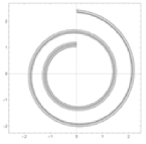
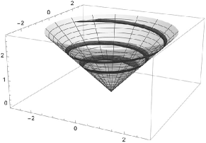
Here is one example to illustrate the structure theorem: We consider the $1/2$ -tubular neighborhood ${\mathcal{U}}$ of the logarithmic spiral (see Figure 2, left)

\gamma(t)=e^{t/15}(\cos t,\sin t)\qquad(\pi/2<t<4\pi+\pi/2)

in the $xy$ -plane, and consider the image $F({\mathcal{U}})$ with respect to the graph $F(x,y):=(x,y,\sqrt{x^{2}+y^{2}})$ . Then $F({\mathcal{U}})$ is an open subset of the light-cone $\Lambda^{2}$ (see Figure 2, right). Since $F({\mathcal{U}})$ is a ruled surface, we can extend each of the ruling light-like lines to both sides, and obtain an $L$ -complete null wave front $\check{F}$ as an $L$ -completion of $F({\mathcal{U}})$ . However, this surface $\check{F}$ is different from the light-cone $\Lambda^{2}$ . In fact, each light-like line as a generator of the ruled surface $\check{F}$ meets $F({\mathcal{U}})$ several times and $\check{F}$ can be regarded as a kind of double covering the light-cone $\Lambda^{2}$ . To produce the actual $\Lambda^{2}$ from the extension of $F({\mathcal{U}})$ , we need to consider the quotient space with an appropriate equivalence relation in the image of $\check{F}$ . In this example, the resulting $L$ -completion is the light-cone $\Lambda^{2}$ , which is, of course, a Hausdorff space. However, in the general situation, in order for the domain of definition of the resulting $L$ -complete null wave front to be a Hausdorff space, it is necessary to assume appropriate conditions on the original null wave front.

From now on, we fix a (co-orientable) null $C^{r}$ -wave front $F:M^{n}\to{\mathbb{R}}^{n+1}_{1}$ which may not be $L$ -complete. Let

(3.1)

\tau:M^{n}\ni p\mapsto\hat{\tau}\circ F(p)\in{\mathbb{R}},

be the restriction of the height function $\hat{\tau}$ to the hypersurface $F$ . he following lemma will play an important role:

Lemma 3.1.

Let $F:M^{n}\to{\mathbb{R}}^{n+1}_{1}$ be a $($ co-orientable $)$ null $C^{r}$ -wave front, and let $p$ be a point in $M^{n}$ . Then, for each open neighborhood $\tilde{U}$ of $p$ , there exist

•

a neighborhood $U(\subset\tilde{U})$ of $p$ ,
•

a positive number $\varepsilon_{U}\in(0,\infty]$ and a real number $t_{U}$ ,
•

a $C^{r}$ -differentiable $(n-1)$ -submanifold $\Sigma_{U}$ of $U$ ,
•

a surjective $C^{r}$ -submersion $\rho_{U}:U\to\Sigma_{U}$ , and
•

a $C^{r}$ -wave front $\tilde{g}_{U}:\Sigma_{U}\to\{0\}\times{\mathbb{R}}^{n}_{0}$

such that

(1)

We set $\hat{\xi}_{U}(x):=\hat{\xi}_{E}|_{\Sigma_{U}}(x)$ $(x\in\Sigma_{U})$ and denote by $\hat{\xi}_{U}=(1,\nu_{U})$ . Then $\nu_{U}(x)$ gives a unit normal vector field of $\tilde{g}_{U}$ in ${\mathbb{R}}^{n}_{0}$ $($ by regarding $\tilde{g}_{U}$ is a map into ${\mathbb{R}}^{n}_{0})$ .

(2)

We set

(3.2)			$\displaystyle G_{U}:{\mathbb{R}}\times\Sigma_{U}\ni(t,x)\mapsto\tilde{g}_{U}(x)+t\hat{\xi}_{U}(x)\in{\mathbb{R}}^{n+1}_{1}\qquad(x\in\Sigma_{U},\,\,t\in{\mathbb{R}}),$
		$\displaystyle\tau_{U}(q):=\tau(q)\qquad(q\in U).$

Then the map given by

\Phi_{U}(q):=(\tau_{U}(q),\rho_{U}(q))\qquad(q\in U)

is a diffeomorphism between $U$ and $I_{U}\times\Sigma_{U}$ satisfying

(3.3)

F(q)=G_{U}\circ\Phi_{U}(q)=\tilde{g}_{U}\circ\rho_{U}(q)+\tau_{U}(q)\hat{\xi}_{U}\circ\rho_{U}(q)\qquad(q\in U),

where $I_{U}:=(-\varepsilon_{U}+t_{U},\varepsilon_{U}+t_{U})$ if $\varepsilon_{U}\neq\infty$ and $I_{U}={\mathbb{R}}$ if $\varepsilon_{U}=\infty$ .

(3)

The map given by

{\mathcal{L}}_{U}:{\mathbb{R}}\times\Sigma_{U}\ni(t,x)\mapsto(G_{U}(t,x),\hat{\xi}_{U}(x))\in{\mathbb{R}}^{n+1}_{1}\times{\mathbb{R}}^{n+1}_{1},

is an embedding satisfying

{\mathcal{L}}_{F}(q)={\mathcal{L}}_{U}\circ\Phi_{U}(q)\qquad(q\in U).

(4)

The map defined by

\tilde{l}_{U}:\Sigma_{U}\ni x\mapsto(\tilde{g}_{U}(x),\hat{\xi}_{U}(x))\in(\{0\}\times{\mathbb{R}}^{n}_{0})\times{\mathbb{R}}^{n+1}_{1}

is an embedding.

In this setting, if $F$ itself is $L$ -complete and $\tilde{U}:=M^{n}$ , then the above assertions hold by setting $I_{U}:={\mathbb{R}}$ .

Definition 3.2.

In this setting, if ${\mathcal{L}}_{U}:{\mathbb{R}}\times\Sigma_{U}\to{\mathbb{R}}^{n+1}_{1}\times{\mathbb{R}}^{n+1}_{1}$ is an embedding, $U$ is called an $F$ -adapted neighborhood of $p$ . Moreover, $(U,\Sigma_{U},\tau_{U},\rho_{U},\tilde{g}_{U},\hat{\xi}_{U},I_{U})$ is called the fundamental $F$ -data at $p$ .

Proof of Lemma 3.1.

Let $\xi_{E}$ be the $E$ -normalized null vector field of $F$ . Since $\hat{\xi}_{E}(\neq{\mathbf{0}})$ points in the light-like future direction, we have $d\tau(\xi_{E})>0$ . In particular, by the implicit function theorem, the level set

\tilde{\Sigma}^{n-1}:=\tau^{-1}(\tau(p))\cap\tilde{U}\,(\subset M^{n})

is an embedded hypersurface of $\tilde{U}$ . We set

(3.4)

t_{0}:=\tau(p).

Since $\xi_{E}$ is transversal to the hypersurface $\tilde{\Sigma}^{n-1}$ , there exist

•

an open interval of the form $J:=(-\varepsilon,\varepsilon)$ ( $\varepsilon>0$ ) or $J:={\mathbb{R}}$ ,
•

a connected open submanifold $\Sigma^{n-1}$ of $\tilde{\Sigma}^{n-1}$ satisfying $p\in\Sigma^{n-1}$ , and
•

an injective $C^{r}$ -immersion

$\tilde{\Psi}:J\times\Sigma^{n-1}\ni(t,x)\mapsto\varphi_{t}(x)\in\tilde{U}$

such that (cf. [2, Proposition A.3]) the map $t\mapsto\varphi_{t}(x)$ ( $x\in\Sigma^{n-1}$ ) gives an integral curve of $\xi_{E}$ satisfying $\varphi_{0}(x)=x$ . In this setting, if $F$ is $L$ -complete and $\tilde{U}=M^{n}$ , then $\xi_{E}$ is a complete vector field of $M^{n}$ and we can set $J:={\mathbb{R}}$ .

Since $\tilde{\Psi}$ is an injective immersion between manifolds of the same dimension, by the inverse function theorem, $\tilde{\Psi}$ is an open map and so

(3.5)

U:=\tilde{\Psi}(J\times\Sigma^{n-1})(\subset\tilde{U})

is a neighborhood of $p$ , and $\tilde{\Psi}$ gives a diffeomorphism from $J\times\Sigma^{n-1}$ to $U$ . Moreover, if $F$ is $L$ -complete and $\tilde{U}:=M^{n}$ , the map $\tilde{\Psi}$ gives a diffeomorphism between ${\mathbb{R}}\times\Sigma^{n-1}$ and $M^{n}$ by the same reason why $\Psi$ is a diffeomorphism in the proof of Theorem 2.6.

We define a map by

\rho:U\ni q\mapsto\pi_{2}\circ\tilde{\Psi}^{-1}(q)\in\Sigma^{n-1},

where $\pi_{2}$ is the canonical projection of $J\times\Sigma^{n-1}$ onto $\Sigma^{n-1}$ . Since $\tau\circ\varphi_{t}(x)=t+t_{0}$ for $x\in\Sigma^{n-1}$ (cf. (3.4)), $\rho$ is a surjective submersion satisfying

(3.6)

\big{(}\tau(q)-t_{0},\rho(q)\big{)}=\tilde{\Psi}^{-1}(q)\qquad(q\in U).

By Theorem 1.14, $F\circ\varphi_{t}(x)$ ( $t\in J$ , $x\in\Sigma^{n-1}$ ) lies on a light-like straight line, and so, the vector $\hat{\xi}_{E}\circ\varphi_{t}(x)\in{\mathbb{R}}^{n+1}_{1}$ does not depend on the parameter $t$ . So we can write

(\hat{\xi}_{E}(x):=)\hat{\xi}_{E}\circ\varphi_{t}(x)=(a(x),\nu(x))\qquad(x\in\Sigma^{n-1}),

where $a(x)>0$ (since $\hat{\xi}_{E}$ points in the future direction). We regard $\hat{\tau}^{-1}(t_{0})$ is a Euclidean $n$ -space. By the same argument as in the proof of Theorem 2.6 (cf. (2.10), (2.11) and (2.12)), we have $a=\pm 1$ and can write

(3.7)

\hat{\xi}_{E}(x)=(1,\nu(x)),\quad|\nu(x)|=1\qquad(x\in\Sigma^{n-1})

such that $(0,\nu)$ gives a unit normal vector field of the map

\tilde{f}:=F|_{\Sigma^{n-1}}:\Sigma^{n-1}\to\hat{\tau}^{-1}(t_{0})(\subset{\mathbb{R}}^{n+1}_{1}).

So $f$ is a frontal in $\hat{\tau}^{-1}(t_{0})$ . Moreover, since $F(\varphi_{t}(x))$ ( $x\in\Sigma^{n-1}$ ) parametrizes a light-like straight line, we have that

(3.8)

F\circ\tilde{\Psi}(t,x)=\tilde{f}(x)+t\hat{\xi}_{E}(x)\qquad(t\in J,\,\,x\in\Sigma^{n-1}).

We next show that $\tilde{f}$ is a wave front in the hyperplane $\hat{\tau}^{-1}(t_{0})$ . Since $F$ is a null wave front in ${\mathbb{R}}^{n+1}_{1}$ , the pair ${\mathcal{L}}_{F}:=(F,\hat{\xi}_{E})$ is an immersion from $M^{n}$ into ${\mathbb{R}}^{n+1}_{1}\times{\mathbb{R}}^{n+1}_{1}$ (cf. Lemma 1.6). By (3.8), we can write

{\mathcal{L}}_{F}\circ\tilde{\Psi}(t,x)=\big{(}\tilde{f}(x)+t\hat{\xi}_{E}(x),\hat{\xi}_{E}(x)\big{)}\qquad((t,x)\in J\times\Sigma^{n-1}).

By setting $\tilde{f}(x)=(t_{0},f(x))$ ( $x\in\Sigma^{n-1}$ ), the rank of the matrix (2.5) for $t=t_{0}$ satisfies

\operatorname{rank}{\begin{pmatrix}1&0&\ldots&0\\ \nu&f_{u_{1}}+t\nu_{u_{1}}&\ldots&f_{u_{n-1}}+t\nu_{u_{n-1}}\\ 0&0&\ldots&0\\ {\mathbf{0}}&\nu_{u_{1}}&\ldots&\nu_{u_{n-1}}\end{pmatrix}}=\operatorname{rank}{\begin{pmatrix}1&0&\ldots&0\\ \nu&f_{u_{1}}&\ldots&f_{u_{n-1}}\\ 0&0&\ldots&0\\ \bf 0&\nu_{u_{1}}&\ldots&\nu_{u_{n-1}}\end{pmatrix}}.

Since the right-hand side is equal to $n$ , the matrix

{\begin{pmatrix}f_{u_{1}}&\ldots&f_{u_{n-1}}\\ \nu_{u_{1}}&\ldots&\nu_{u_{n-1}}\end{pmatrix}}

is of rank $n-1$ at each point of $\Sigma^{n-1}$ . So $\tilde{f}$ is a wave front on $\Sigma^{n-1}$ .

We consider the map $\tilde{g}:\Sigma^{n-1}\to\hat{\tau}^{-1}(0)$ given by

\tilde{g}(x):=\tilde{f}(x)-t_{0}\hat{\xi}_{E}(x)\qquad(x\in\Sigma^{n-1}),

which corresponds to the parallel hypersurface of $f$ having signed equi-distance $-t_{0}$ in ${\mathbb{R}}^{n}_{0}$ . Then $\tilde{g}$ is a wave front in $\hat{\tau}^{-1}(0)$ whose unit normal vector field $\nu$ satisfies

(1,\nu(x))=\hat{\xi}_{E}|_{\Sigma^{n-1}}(x)\qquad(x\in\Sigma^{n-1}).

Then, by Theorem 2.3,

(3.9)

G(t,x):=\tilde{g}(x)+t(1,\nu(x))\qquad(x\in\Sigma^{n-1},\,\,t\in{\mathbb{R}})

is an $L$ -complete null wave front. We set

I_{U}:=\begin{cases}(-\varepsilon+t_{0},\varepsilon+t_{0})&\text{if $\varepsilon\neq\infty$},\\ {\mathbb{R}}&\text{if $\varepsilon=\infty$},\end{cases}

and consider the following diffeomorphism

\Upsilon:I_{U}\times\Sigma^{n-1}\ni(t,x)\mapsto(t-t_{0},x)\in J\times\Sigma^{n-1}.

By (3.6), it holds that

(3.10)

q=\tilde{\Psi}(\tau(q)-t_{0},\rho(q))=\tilde{\Psi}\circ\Upsilon(\tau(q),\rho(q))\qquad(q\in U).

By this with (3.8) and (3.9), we have

	$\displaystyle F(q)$	$\displaystyle=F\circ\tilde{\Psi}\circ\Upsilon(\tau(q),\rho(q))=F\circ\tilde{\Psi}(\tau(q)-t_{0},\rho(q))$
		$\displaystyle=\tilde{f}\circ\rho(q)+(\tau(q)-t_{0})\hat{\xi}_{E}\circ\rho(q)$
		$\displaystyle=\tilde{g}\circ\rho(q)+\tau(q)\hat{\xi}_{E}\circ\rho(q)=G(\tau(q),\rho(q))$

for each $q\in U$ . Thus, by setting

	$\displaystyle\Phi_{U}:=(\tilde{\Psi}\circ\Upsilon)^{-1},\quad\varepsilon_{U}:=\varepsilon,\quad t_{U}:=t_{0},\quad\rho_{U}:=\rho,$
	$\displaystyle\nu_{U}:=\nu,\quad\hat{\xi}_{U}:=(1,\nu_{U}),\quad\Sigma_{U}:=\Sigma^{n-1},\quad G_{U}:=G,\quad\tilde{g}_{U}:=\tilde{g},$

we obtain the desired fundamental data: In fact, if we set

	$\displaystyle{\mathcal{L}}_{U}:{\mathbb{R}}\times\Sigma^{n-1}\ni(t,x)\mapsto\big{(}G_{U}(t,x),\hat{\xi}_{U}(x)\big{)}\in{\mathbb{R}}^{n+1}_{1}\times{\mathbb{R}}^{n+1}_{1},$
	$\displaystyle\tilde{l}_{U}:\Sigma^{n-1}\ni x\mapsto\big{(}\tilde{g}_{U}(x),\hat{\xi}_{U}(x)\big{)}\in(\{0\}\times{\mathbb{R}}^{n}_{0})\times{\mathbb{R}}^{n+1}_{1},$

then the two maps $\tilde{l}_{U}$ and ${\mathcal{L}}_{U}$ are immersions, since we have already shown that $\tilde{g}_{U}$ and $G_{U}$ are wave fronts.

Since every immersion is locally an embedding, if we choose the open neighborhood $U(\subset\tilde{U})$ of $p$ to be sufficiently small (that is, we choose a sufficiently small $\Sigma^{n-1}$ , see (3.5)), then $\tilde{l}_{U}$ gives an embedding. Then, by Lemma 2.5, ${\mathcal{L}}_{U}$ is also an embedding. ∎

By Lemma 3.1, for each point $p\in M^{n}$ , there exist fundamental $F$ -data

(U_{p},\Sigma_{p},\tau_{p},\rho_{p},\tilde{g}_{p},\hat{\xi}_{p},I_{p})

such that $U_{p}$ is an $F$ -adapted neighborhood of $p$ giving an $L$ -complete null wave front (cf. (3.2))

G_{p}:{\mathbb{R}}\times\Sigma_{p}\ni(t,x)\mapsto\tilde{g}_{p}(x)+t\hat{\xi}_{p}(x)\in{\mathbb{R}}^{n+1}_{1}

and an embedding

(3.11)

\tilde{l}_{p}:\Sigma_{p}\ni x\mapsto(\tilde{g}_{p}(x),\hat{\xi}_{p}(x))\in(\{0\}\times{\mathbb{R}}^{n}_{0})\times{\mathbb{R}}^{n+1}_{1}\subset{\mathbb{R}}^{n+1}_{1}\times{\mathbb{R}}^{n+1}_{1},

where $\hat{\xi}_{p}(x)=(1,\nu_{p}(x))$ . Since $M^{n}$ satisfies the second axiom of the countability, there exist an at most countable set ${\mathcal{A}}$ and a family of fundamental $F$ -data

\{(U_{\lambda},\Sigma_{\lambda},\tau_{\lambda},\rho_{\lambda},\tilde{g}_{\lambda},\hat{\xi}_{\lambda},I_{\lambda})\}_{\lambda\in{\mathcal{A}}}

such that

(1)

for each $\lambda\in{\mathcal{A}}$ , there exists $p_{\lambda}\in U_{\lambda}$ satisfying

	$\displaystyle(U_{\lambda},\Sigma_{\lambda},\tau_{\lambda},\rho_{\lambda},\tilde{g}_{\lambda},\hat{\xi}_{\lambda},I_{\lambda}):=(U_{p},\Sigma_{p_{\lambda}},\tau_{p_{\lambda}},\rho_{p_{\lambda}},\tilde{g}_{p_{\lambda}},\hat{\xi}_{p_{\lambda}},I_{p_{\lambda}}),$
	$\displaystyle\tilde{g}_{\lambda}:=\tilde{g}_{p_{\lambda}},$

(2)

the map $\tilde{l}_{\lambda}:\Sigma_{\lambda}\to{\mathbb{R}}^{n+1}_{1}\times{\mathbb{R}}^{n+1}_{1}$ defined by

$\tilde{l}_{\lambda}(x):=(\tilde{g}_{\lambda}(x),\hat{\xi}_{\lambda}(x))\qquad(\lambda\in{\mathcal{A}})$

is an embedding (cf. (4) of Lemma 3.1),
(3)

$M^{n}=\bigcup_{\lambda\in{\mathcal{A}}}U_{\lambda}$ .

In particular, $\{(\Sigma_{\lambda},\tilde{l}_{\lambda})\}_{\lambda\in{\mathcal{A}}}$ is a family of embeddings defined on $(n-1)$ -dimensional manifolds. To ensure that the domain of definition of the resulting $\check{F}$ is a Hausdorff space, we give the following definition:

Definition 3.3.

In the above setting, $F$ is said to be admissible if $\{(\Sigma_{\lambda},\tilde{l}_{\lambda})\}_{\lambda\in{\mathcal{A}}}$ is an admissible family as in Definition B.6 in Appendix B.

We prove the following:

Theorem 3.4 (A structure theorem of null wave fronts).

Let $F:M^{n}\to{\mathbb{R}}^{n+1}_{1}$ be an admissible null $C^{r}$ -wave front $($ if $F$ is real analytic, i.e. $r=\omega$ , it is admissible, see Lemma B.5 $)$ . Then there exist

•

a $C^{r}$ -differentiable $(n-1)$ -manifold $\check{\Sigma}^{n-1}$ ,
•

a $C^{r}$ -immersion ${\mathcal{I}}:M^{n}\to{\mathbb{R}}\times\check{\Sigma}^{n-1}$ ,
•

an $L$ -complete null wave front $\check{F}:{\mathbb{R}}\times\check{\Sigma}^{n-1}\to{\mathbb{R}}^{n+1}_{1}$ written in the normal form and its canonical lift $\check{{\mathcal{L}}}:{\mathbb{R}}\times\check{\Sigma}^{n-1}\to{\mathbb{R}}^{n+1}_{1}\times{\mathbb{R}}^{n+1}_{1}$

such that

\check{F}\circ{\mathcal{I}}(q)=F(q),\qquad\check{{\mathcal{L}}}\circ{\mathcal{I}}(q)={\mathcal{L}}_{F}(q)\qquad(q\in M^{n}).

If ${\mathcal{L}}_{F}$ is an embedding $($ see Remark 3.5 $)$ , then ${\mathcal{I}}$ gives a diffeomorphism between $M^{n}$ and ${\mathcal{I}}(M^{n})$ . Moreover, if $F$ is $L$ -complete, then ${\mathcal{I}}$ is a surjection.

Remark 3.5.

Since $F$ is a null wave front, its canonical lift ${\mathcal{L}}_{F}$ is an immersion. So, the assumption that ${\mathcal{L}}_{F}$ is an embedding is not so restrictive. On the other hand, even if ${\mathcal{L}}_{F}$ is an embedding, the admissibility of $F$ does not hold in general, see Example 3.7.

Proof.

We consider the disjoint union $\mathcal{S}:=\coprod_{\lambda\in{\mathcal{A}}}\Sigma_{\lambda},$ and give a relation $x\sim y$ for $x,y\in\mathcal{S}$ so that $x\sim y$ implies that there exists a pair $(\lambda,\mu)\in{\mathcal{A}}\times{\mathcal{A}}$ of indices such that

•

$\Sigma_{\lambda}$ is a neighborhood of $x$ ,
•

$\Sigma_{\mu}$ is a neighborhood of $y$ , and
•

$x$ is $(\tilde{l}_{\lambda},\tilde{l}_{\mu})$ -related to $y$ in the sense of Definition B.1.

As seen in the proof of Proposition B.7, the symbol $\sim$ gives an equivalence relation, and $\check{\Sigma}^{n-1}:=\mathcal{S}/{\sim}$ is an $(n-1)$ -manifold. Then $\pi:\mathcal{S}\to\check{\Sigma}^{n-1}$ is the canonical projection as an open map. We set

\varphi_{\lambda}:=\pi|_{\Sigma_{\lambda}}.

Then $\{(\Sigma_{\lambda},\varphi_{\lambda})\}_{\lambda\in{\mathcal{A}}}$ is the differentiable structure of $\check{\Sigma}^{n-1}$ as shown in the proof of Proposition B.7. Moreover, an immersion $\check{l}:\check{\Sigma}^{n-1}\to{\mathbb{R}}^{n+1}_{1}\times{\mathbb{R}}^{n+1}_{1}$ is induced which satisfies

\check{l}\circ\varphi_{\lambda}(x)=(\tilde{g}_{\lambda},\hat{\xi}_{\lambda})(=\tilde{l}_{\lambda})\qquad(x\in\Sigma_{\lambda},\,\,\lambda\in{\mathcal{A}}).

We can write

\check{l}(\check{x})=(\tilde{g}(\check{x}),\hat{\xi}(\check{x}))\qquad(\check{x}\in\check{\Sigma}^{n-1}).

Then, by definition, we have

\tilde{g}\circ\varphi_{\lambda}(x)=\tilde{g}_{\lambda}(x),\quad\hat{\xi}\circ\varphi_{\lambda}(x)=\hat{\xi}_{\lambda}(x)\qquad(x\in\Sigma_{\lambda})

So, if we set

	$\displaystyle\check{F}(t,\check{x})$	$\displaystyle:=\tilde{g}(\check{x})+t\hat{\xi}(\check{x})\qquad((t,\check{x})\in{\mathbb{R}}\times\check{\Sigma}^{n-1}),$
	$\displaystyle G_{\lambda}(t,x)$	$\displaystyle:=\tilde{g}_{\lambda}(x)+t\hat{\xi}_{\lambda}(x)\qquad(t\in{\mathbb{R}},\,x\in\Sigma_{\lambda}),$

then it holds that

(3.12)		$\displaystyle\check{F}(t,\varphi_{\lambda}(x))$	$\displaystyle=\tilde{g}\circ\varphi_{\lambda}(x)+t\hat{\xi}\circ\varphi_{\lambda}(x)$
		$\displaystyle=\tilde{g}_{\lambda}(x)+t\hat{\xi}_{\lambda}(x)=G_{\lambda}(t,x)$

for $t\in{\mathbb{R}}$ and $x\in\Sigma_{\lambda}$ . So, if we consider the maps defined by

	$\displaystyle\check{{\mathcal{L}}}:{\mathbb{R}}\times\check{\Sigma}^{n-1}\ni(t,\check{x})\mapsto\Big{(}\tilde{g}(\check{x})+t\hat{\xi}(\check{x}),\hat{\xi}(\check{x})\Big{)}\in{\mathbb{R}}^{n+1}_{1}\times{\mathbb{R}}^{n+1}_{1},$
	$\displaystyle{\mathcal{L}}_{\lambda}:{\mathbb{R}}\times\Sigma_{\lambda}\ni(t,x)\mapsto\big{(}G_{\lambda}(t,x),\hat{\xi}_{\lambda}(x)\big{)}\in{\mathbb{R}}^{n+1}_{1}\times{\mathbb{R}}^{n+1}_{1},$

then we have

\check{{\mathcal{L}}}(t,\varphi_{\lambda}(x))={\mathcal{L}}_{\lambda}(t,x)\qquad(t\in{\mathbb{R}},\,\,x\in\Sigma_{\lambda}).

We set

\check{\Sigma}_{\lambda}:=\varphi_{\lambda}(\Sigma_{\lambda}).

Since ${\mathcal{L}}_{\lambda}$ is an embedding (see (3) of Lemma 3.1), then the restriction $\check{{\mathcal{L}}}|_{{\mathbb{R}}\times\check{\Sigma}_{\lambda}}$ is also an embedding for each $\lambda\in\mathcal{A}$ . In particular, $\check{F}$ is an $L$ -complete null wave front on ${\mathbb{R}}\times\check{\Sigma}^{n-1}$ .

We then fix $p\in M^{n}$ arbitrarily, and assume that $p$ belongs to $U_{\lambda}$ for some $\lambda\in{\mathcal{A}}$ . By (3.3) and (3.12), we have

	$\displaystyle F(q)$	$\displaystyle=\tilde{g}_{\lambda}\circ\rho_{\lambda}(q)+\tau_{\lambda}(q)\,\hat{\xi}_{\lambda}\circ\rho_{\lambda}(q)$
		$\displaystyle=G_{\lambda}(\rho_{\lambda}(q),\tau_{\lambda}(q))=\check{F}(\tau_{\lambda}(q),\varphi_{\lambda}\circ\rho_{\lambda}(q))\qquad(q\in U_{\lambda}).$

So it holds that

(3.13)

{\mathcal{L}}_{F}(q)=\check{{\mathcal{L}}}(\tau_{\lambda}(q),\varphi_{\lambda}\circ\rho_{\lambda}(q))\qquad(q\in U_{\lambda}).

Since ${\mathcal{L}}_{F}$ and $\check{{\mathcal{L}}}$ are immersions, the map

(3.14)

{\mathcal{I}}_{\lambda}:U_{\lambda}\ni q\mapsto(\tau_{\lambda}(q),\varphi_{\lambda}\circ\rho_{\lambda}(q))\in{\mathbb{R}}\times\check{\Sigma}_{\lambda}

is also an immersion.

If $p\in U_{\mu}$ for some other index $\mu\in{\mathcal{A}}$ , then the immersion ${\mathcal{I}}_{\mu}:U_{\mu}\to{\mathbb{R}}\times\check{\Sigma}_{\mu}$ is also induced. Since $\check{{\mathcal{L}}}|_{{\mathbb{R}}\times\check{\Sigma}_{\lambda}}$ and $\check{{\mathcal{L}}}|_{{\mathbb{R}}\times\check{\Sigma}_{\mu}}$ are embeddings, so is $\check{{\mathcal{L}}}|_{{\mathbb{R}}\times(\check{\Sigma}_{\lambda}\cap\check{\Sigma}_{\mu})}$ . Thus ${\mathcal{I}}_{\lambda}$ coincides with ${\mathcal{I}}_{\mu}$ on $U_{\lambda}\cap U_{\mu}$ , and the map ${\mathcal{I}}:M^{n}\to{\mathbb{R}}\times\check{\Sigma}^{n-1}$ is canonically induced. By (3.13) and (3.14),

{\mathcal{L}}_{F}(q)=\check{{\mathcal{L}}}\circ{\mathcal{I}}(q)\qquad(q\in M^{n})

holds. In particular, $\check{F}\circ{\mathcal{I}}=F$ also holds on $M^{n}$ . We now consider the case that ${\mathcal{L}}_{F}$ is an embedding. Suppose that ${\mathcal{I}}(p)={\mathcal{I}}(q)$ ( $p,q\in M^{n}$ ). Then we have

{\mathcal{L}}_{F}(p)=\check{{\mathcal{L}}}\circ{\mathcal{I}}(p)=\check{{\mathcal{L}}}\circ{\mathcal{I}}(q)={\mathcal{L}}_{F}(q).

Since ${\mathcal{L}}_{F}$ is an embedding, we have $p=q$ , proving the injectivity of ${\mathcal{I}}$ . Since ${\mathcal{I}}$ is an immersion between same dimensional manifolds, it is a diffeomorphism.

If $F$ is $L$ -complete, then $\tau_{\lambda}(U_{\lambda})={\mathbb{R}}$ and $\rho_{\lambda}(U_{\lambda})=\Sigma_{\lambda}$ for each $\lambda\in{\mathcal{A}}$ , which imply that the map ${\mathcal{I}}_{\lambda}$ is surjective (cf. (3.14)). So we can conclude that ${\mathcal{I}}$ is a surjection. ∎

Example 3.6.

We set ${\mathbb{R}}^{2}_{*}:={\mathbb{R}}^{2}\setminus\{(0,0)\}$ , and consider a null immersion

F:{\mathbb{R}}^{2}_{*}\ni(u,v)\mapsto(u^{2}+v^{2},2uv,u^{2}-v^{2})\in({\mathbb{R}}^{3}_{1};t,x,y),

whose image lies on the light-cone $\Lambda^{2}$ passing through the origin in ${\mathbb{R}}^{3}_{1}$ . In this case, the image of the $L$ -completion of $F$ is the light-cone $\Lambda^{2}$ and so the map $F$ covers twice on $\Lambda^{2}\cap\{t>0\}$ in ${\mathbb{R}}^{3}_{1}$ . In particular, the induced map ${\mathcal{I}}$ is not a diffeomorphism. This example shows that if we drop the condition that ${\mathcal{L}}_{F}$ is injective, the injectivity of $\Phi$ does not follow, in general.

Example 3.7.

Consider a plane curve (cf. Figure 3)

\gamma(t):=e^{\omega(t)}(\cos t,\sin t)\qquad(0\leq t\leq 4\pi),

where $\omega(t)$ is a $C^{\infty}$ -function into $[0,1]$ such that $\omega(t)=0$ for $t\not\in(3\pi-\varepsilon,3\pi+\varepsilon)$ and $\omega(t)>0$ for $t\in(3\pi-\varepsilon,3\pi+\varepsilon)$ , where $\varepsilon$ is a sufficiently small positive number. Then $\gamma$ generates the $L$ -complete null wave front $\mathcal{F}^{\gamma}_{+}$ (cf. Theorem 2.3). By the construction of $\gamma$ , $\mathcal{F}^{\gamma}_{+}$ is not admissible, since the image of $\mathcal{F}^{\gamma}_{+}$ has non-transversal intersections. We then set

\Gamma(t):=(0,\gamma(t))+t(1,\nu(t))\qquad(0\leq t\leq 4\pi),

where $\nu(t)$ is a unit normal vector field of $\gamma(t)$ . The image $C:=\Gamma([0,4\pi])$ of $\Gamma$ is an embedded spiral-shaped curve on image of $\mathcal{F}^{\gamma}_{+}$ . Consider a sufficiently small tubular neighborhood ${\mathcal{U}}_{C}$ of $C$ in the image of $\mathcal{F}^{\gamma}_{+}$ . Then ${\mathcal{U}}_{C}$ is an embedded null surface, because $\Gamma$ has no self-intersections. If we think that $F$ is the inclusion map ${\mathcal{U}}_{C}\hookrightarrow{\mathbb{R}}^{3}_{1}$ , then the $L$ -completion of $F$ is $\mathcal{F}^{\gamma}_{+}$ . So, this example shows that the admissibility of the $L$ -completion of $F$ in Theorem 3.4 is independent of the embeddedness of the canonical lift ${\mathcal{L}}_{F}$ .

Moreover, if we apply our $L$ -completion procedure for ${\mathcal{U}}_{C}$ , then the resulting quotient space is not a Hausdorff space, which implies the necessity of the admissibility condition as in Definition 3.3.

4. Classification of complete null wave fronts

In this section, we define “completeness” of null wave fronts and prove a structure theorem of them. The content of this section is completely independent of Section 3.

Definition 4.1.

A null $C^{r}$ -wave front $F:M^{n}\to{\mathbb{R}}^{n+1}_{1}$ is said to be complete if

•

$F$ is $L$ -complete, and
•

the singular set of $F$ is a non-empty compact subset of $M^{n}$ .

Remark 4.2.

As proved in [2], if $F$ is $L$ -complete and its singular set is empty, then the image $F(M^{n})$ is a subset of a light-like hyperplane of ${\mathbb{R}}^{n+1}_{1}$ , which is a trivial case. So we only consider the case that the singular set of $F$ is non-empty, in the above definition.

Remark 4.3.

When $n=2$ , a null wave front $F$ in ${\mathbb{R}}^{3}_{1}$ is a surface with vanishing Gaussian curvature (cf. [1, Appendix]). If $F$ is complete, then it is complete as a flat front in the Euclidean 3-space in the sense of Murata-Umehara [9].

We prove the following:

Theorem 4.4.

Let $F$ be a null $C^{r}$ -wave front in ${\mathbb{R}}^{n+1}_{1}$ . If $F$ is complete, then it can be reparametrized as a normal form ${\mathcal{F}}^{f}_{+}$ , where $f:\Sigma^{n-1}\to{\mathbb{R}}^{n}_{0}$ is an immersion defined on a compact $(n-1)$ -manifold $\Sigma^{n-1}$ whose principal curvatures are non-zero and all same sign everywhere in ${\mathbb{R}}^{n}_{0}$ . In particular, if $n\geq 3$ , then $f$ is a compact convex hypersurface in ${\mathbb{R}}^{n}_{0}$ . On the other hand, if $n=2$ , then $f$ is a closed locally convex regular curve in ${\mathbb{R}}^{2}_{0}$ .

Proof.

We let $F:M^{n}\to{\mathbb{R}}^{n+1}_{1}$ be a complete null wave front. By Theorem 2.6, we may assume that there exist

•

an $(n-1)$ -manifold $\Sigma^{n-1}$ ,
•

a diffeomorphism $\Phi:M^{n}\to{\mathbb{R}}\times\Sigma^{n-1}$ , and
•

a co-orientable wave front $f:\Sigma^{n-1}\to{\mathbb{R}}^{n}_{0}$

such that $F\circ\Phi^{-1}$ coincides with the normal form ${\mathcal{F}}^{f}_{+}$ given in Theorem 2.3. We consider the height function $\hat{\tau}:{\mathbb{R}}^{n+1}_{1}\to{\mathbb{R}}$ given in (2.1). Since the singular set of $F$ is compact, for sufficiently large $t_{0}$ , the restriction

\tilde{f}:=F\circ\Phi^{-1}|_{\Phi(\tau^{-1}(t_{0}))}:\Sigma^{n-1}\to\hat{\tau}^{-1}(t_{0})

is an immersion such that $\tilde{f}(x)=(t_{0},f(x))$ . Without loss of generality, we may assume that $t_{0}=0$ and $F$ satisfies

(4.1)

F\circ\Phi^{-1}(t,x)=\tilde{f}(x)+t\hat{\xi}_{E}(x),\quad\hat{\xi}_{E}(x):=(1,\nu(x))\qquad(t\in{\mathbb{R}},\,\,x\in\Sigma^{n-1}),

where $\nu$ can be considered as the unit normal vector field along the immersion $f$ . So, we may assume that $F$ is defined on ${\mathbb{R}}\times\Sigma^{n-1}$ . Since $f$ is co-orientable and is an immersion, $\Sigma^{n-1}$ is orientable. We let

\lambda_{1}\leq\cdots\leq\lambda_{n-1}

be principal curvature functions of $f$ . Here, $\{\lambda_{i}(x)\}_{i=1}^{n-1}$ are eigenvalues of a symmetric matrix associated with the shape operator of $f$ at $x$ . Since the characteristic polynomial of a real symmetric matrix consists only of real roots, the well-known fact that the roots of a polynomial depend continuously on its coefficients implies that $\{\lambda_{i}\}_{i=1}^{n-1}$ can be considered as a family of real-valued continuous functions defined on $\Sigma^{n-1}$ . We first show that each $\lambda_{i}$ never changes sign: Suppose that there exists a sequence of points $\{x_{k}\}_{k=1}^{\infty}$ which converges to a point $x_{\infty}$ such that

\lambda_{i}(x_{k})\neq 0\,\,\text{ and }\,\,\lambda_{i}(x_{\infty})=0.

Then

\left(\frac{1}{\lambda_{i}(x_{k})},x_{k}\right)\in{\mathbb{R}}\times\Sigma^{n-1}\qquad(k=1,2,3,\ldots)

are singular points of $F$ which are unbounded on ${\mathbb{R}}\times\Sigma^{n-1}$ , contradicting the compactness of the singular set of $F$ . Thus, each $\lambda_{i}$ as a continuous function on $\Sigma^{n-1}$ has no zeros unless it is identically zero. By Remark 4.2, $f$ is not a part of a hyperplane in ${\mathbb{R}}^{n}_{0}$ . So, there exists an integer $r$ ( $1\leq r\leq n-1$ ) such that $\lambda_{i_{s}}\,\,(s=1,\ldots,r)$ are not identically zero, where $\{i_{1},\ldots,i_{r}\}$ is a subset of $\{1,\ldots,n-1\}$ . By Hartman’s product theorem (cf. [8, Page 347]), $\Sigma^{n-1}$ is a product of a compact manifold and ${\mathbb{R}}^{l}$ ( $l:=n-1-r$ ). For each $s\in\{1,\ldots,r\}$ , we can define a continuous map $\psi_{s}:\Sigma^{n-1}\to{\mathbb{R}}\times\Sigma^{n-1}$ by

\psi_{s}(x):=\left(\frac{1}{\lambda_{i_{s}}(x)},x\right)\in{\mathbb{R}}\times\Sigma^{n-1}.

Then $S:=\bigcup_{s=1}^{r}\psi_{s}(\Sigma^{n-1})$ coincides with the singular set of $F$ . Since $F$ is complete null wave front, $S$ is compact. Since the projection of $S$ via the continuous map

{\mathbb{R}}\times\Sigma^{n-1}\ni(t,x)\mapsto x\in\Sigma^{n-1}

is compact, the hypersurface $\Sigma^{n-1}$ is also compact. Thus $r=n-1$ (i.e. $l=0$ ) and each $\lambda_{i}$ ( $i=1,\ldots,n-1$ ) is either positive-valued or negative-valued on $\Sigma^{n-1}$ . Moreover, since $\Sigma^{n-1}$ is compact, there exists a point $y_{0}\in\Sigma^{n-1}$ such that $f(y_{0})$ attains the farthest point of the image of $f$ from the origin in ${\mathbb{R}}^{n}_{0}$ . Then $\lambda_{1}(y_{0}),\,\,\dots,\,\,\lambda_{n-1}(y_{0})$ are all positive or all negative at the same time.

Here, replacing $\nu$ by $-\nu$ , we may assume that

\lambda_{n-1}(x)>0\qquad(x\in\Sigma^{n-1}).

Then, $\lambda_{1},\dots,\lambda_{n-1}$ take the same sign on $\Sigma^{n-1}$ . Thus, Hadamard’s theorem [5] implies that $f$ is an embedded convex hypersurface in ${\mathbb{R}}^{n}_{0}$ whenever $n\geq 3$ . ∎

If $n=2$ , then $f$ is a locally strictly convex regular curve in ${\mathbb{R}}^{2}_{0}$ . So we may express $f$ by $\gamma(s)$ $(s\in{\mathbb{R}})$ defined as an $l$ -periodic curve ( $l>0$ ), parametrized by the arc-length. Then its curvature function can be taken so that $\kappa(s)$ is positive everywhere. Then we may assume that $F$ is expressed as

F(t,s)=(t,\gamma_{t}(s))\qquad(s,t\in{\mathbb{R}}),

where $\gamma_{t}(s):=\gamma(s)+t\nu(s)$ is a parallel curve of $\gamma$ , and the singular set of $F$ is

S:=\{(1/\kappa(s),s)\,;\,s\in{\mathbb{R}}\},

and

(4.2)

C_{\gamma}(s):=F\left(\frac{1}{\kappa(s)},s\right)

just parametrizes the singular set image of $F$ . We can prove the following:

Proposition 4.5.

Let $F$ be a complete null wave front in ${\mathbb{R}}^{3}_{1}$ which is generated by a closed locally convex regular curve $\gamma$ in ${\mathbb{R}}^{2}_{0}$ . Then non-cuspidal edge points of $F$ correspond to vertices on $\gamma$ , where a vertex is a critical point of the curvature function of $\gamma$ .

Proof.

In the setting of (4.2), $C^{\prime}_{\gamma}(s)\neq{\mathbf{0}}$ if and only if $\kappa^{\prime}(s_{0})\neq 0$ , and so $F$ has a cuspidal edge singular point at $(1/\kappa(s_{0}),s_{0})$ only when $\kappa^{\prime}(s_{0})\neq 0$ (see the criterion in [3] for cuspidal edge). ∎

The following assertion is equivalent to the classical four vertex theorem for convex plane curve:

Corollary 4.6.

Let $F$ be a complete null wave front in ${\mathbb{R}}^{3}_{1}$ which has no self-intersections outside of a compact subset of ${\mathbb{R}}^{3}_{1}$ . Then $F$ has at least four non-cuspidal edge singular points.

Proof.

Since $F$ has no self-intersections outside of a compact set, $F$ must be generated by a (closed) convex plane curve $\gamma$ in the $xy$ -plane. By the classical four vertex theorem, $\gamma$ has at least four vertices, then such points corresponds to the non-cuspidal edge points of $F$ as seen in the proof of Proposition 4.5. So we obtain the assertion. ∎

Since a complete null wave front in ${\mathbb{R}}^{3}_{1}$ can be considered as a complete flat front in the Euclidean $3$ -space, Corollary 4.6 is a special case of the four non-cuspidal edge point theorem given in [9, Theorem D].

Example 4.7.

We consider the complete null wave front $F_{a}$ associated with the ellipse as in the introduction which has four vertices when $0<a<1$ . They correspond to the swallowtail singular points of the complete null wave front in Figure 1 in the introduction, which satisfies the assumption of Corollary 4.6.

Example 4.8.

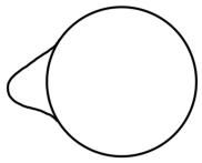
Consider a locally convex plane curve with a self-intersection

\gamma(\theta):=(1-2\sin\theta)(\cos\theta,\sin\theta)\qquad(0\leq\theta\leq 2\pi),

which admits only two vertices. These vertices correspond to two swallowtail singular points of the corresponding null wave front as in Figure 4.

Appendix A A lemma of subspaces in ${\mathbb{R}}^{n+1}_{1}$

We denote by $\left\langle{},{}\right\rangle$ the canonical Lorentzian inner product of ${\mathbb{R}}^{n+1}_{1}$ . In this section, we prepare the following assertion for vector subspaces in ${\mathbb{R}}^{n+1}_{1}$ .

Definition A.1.

A subspace $V$ of ${\mathbb{R}}^{n+1}_{1}$ is said to be perpendicular to a subspace $W$ if $\left\langle{{\mathbf{v}}},{{\mathbf{w}}}\right\rangle=0\,\,({\mathbf{v}}\in V,\,\,{\mathbf{w}}\in W)$ holds.

For a subspace $V$ of ${\mathbb{R}}^{n+1}_{1}$ , we set

(A.1)

V^{\perp}:=\{{\mathbf{x}}\in{\mathbb{R}}^{n+1}_{1}\,;\,\left\langle{{\mathbf{x}}},{{\mathbf{v}}}\right\rangle=0\,\,\text{for all ${\mathbf{v}}\in V$}\},

which is the maximal subspace perpendicular to $V$ in ${\mathbb{R}}^{n+1}_{1}$ .

Definition A.2.

A subspace $V$ of ${\mathbb{R}}^{n+1}_{1}$ is said to be degenerate if there exists a non-zero vector ${\mathbf{v}}\in V$ such that $\left\langle{{\mathbf{v}}},{{\mathbf{w}}}\right\rangle=0$ for all ${\mathbf{w}}\in V$ . We call such a vector ${\mathbf{v}}$ a degenerate vector of $V$ . On the other hand, a subspace $V(\subset{\mathbb{R}}^{n+1}_{1})$ is said to be non-degenerate if it is not degenerate.

Lemma A.3.

Let $V,W$ and $N$ be three subspaces of ${\mathbb{R}}^{n+1}_{1}$ such that

(1)

$N$ is a 1-dimensional degenerate subspace satisfying $N\cap W=\{{\mathbf{0}}\}$ ,
(2)

$V$ and $W$ are perpendicular to $N$ , and
(3)

$W$ is perpendicular to $V$ .

Then $V\cap W=\{{\mathbf{0}}\}$ .

Proof.

If $W$ is non-degenerate, then so is $W^{\perp}$ , and using (3), we have

\{{\mathbf{0}}\}=W^{\perp}\cap W\supset V\cap W,

which implies $V\cap W=\{{\mathbf{0}}\}$ . So we may assume that $W$ is degenerate. By definition, there exists a degenerate vector ${\mathbf{v}}_{0}$ belonging to $W$ . We let $\xi\in N\setminus\{{\mathbf{0}}\}$ be a generator of the 1-dimensional vector $N$ . Then ${\mathbf{v}}_{0}$ and $\xi$ are both degenerate vectors. In particular, they are light-like, that is, $\left\langle{{\mathbf{v}}_{0}},{{\mathbf{v}}_{0}}\right\rangle=\left\langle{\xi},{\xi}\right\rangle=0$ hold. So if we set $\tilde{W}:=W+N$ , then by (1), $\tilde{W}$ contains two linearly independent light-like vectors ${\mathbf{v}}_{0}$ and $\xi$ , and so, $\tilde{W}$ is a time-like vector space (cf. [10, Lemma 27, Page 141]), which is non-degenerate. So, $\tilde{W}^{\perp}$ is also non-degenerate. Since $V\subset\tilde{W}^{\perp}$ (cf. (2) and (3)) and $W\subset\tilde{W}$ , we have

\{{\mathbf{0}}\}=\tilde{W}^{\perp}\cap\tilde{W}\supset V\cap W,

proving $V\cap W=\{{\mathbf{0}}\}$ . ∎

Appendix B A method to make an immersion defined on a connected manifold from a family of embeddings.

Definition B.1.

We fix positive integers $n,m$ ( $n<m$ ). Let $U,V$ be two connected $n$ -dimensional manifolds. We let $f:U\to{\mathbb{R}}^{m}$ and $g:V\to{\mathbb{R}}^{m}$ be two $C^{r}$ -embeddings. A point $x\in U$ is said to be $(f,g)$ -related to $y\in V$ if there exist an open neighborhood $O_{x}(\subset U)$ of $x$ and an open neighborhood $O_{y}(\subset V)$ of $y$ such that

•

$f(x)=g(y)$ and
•

$f(O_{x})=g(O_{y})$ .

If there are no $(f,g)$ -related points on $U$ and $V$ , we say that “ $U$ is not $(f,g)$ -related to $V$ ”.

Remark B.2.

This “ $(f,g)$ -relatedness” is an open condition. In fact, if $x\in U$ is $(f,g)$ -related to $y\in V$ , then there exist open neighborhoods $O_{x}(\subset U)$ and $O_{y}(\subset V)$ of $x$ and $y$ respectively such that each point of $O_{x}$ is $(f,g)$ -related to a certain point in $O_{y}$ .

In this setting, the following assertion holds.

Lemma B.3.

If we set

	$\displaystyle O_{U,V}$	$\displaystyle:=\{x\in U\,;\,\text{$x$ is $(f,g)$-related to some $y\in V$}\},$
	$\displaystyle O_{V,U}$	$\displaystyle:=\{y\in V\,;\,\text{$y$ is $(g,f)$-related to some $x\in U$}\},$

then $O_{U,V}$ $($ resp. $O_{V,U})$ is an open subset of $U$ $($ resp. $V)$ . Moreover, if $O_{U,V}$ is non-empty, then there exists a unique $C^{r}$ -diffeomorphism $\varphi:O_{U,V}\to O_{V,U}$ satisfying $g\circ\varphi=f$ on $O_{U,V}$ .

Proof.

Assume that $x\in U$ (resp. $y\in V$ ) is $(f,g)$ -related to $y\in V$ (resp. $x\in U$ ). Since $f$ and $g$ are embeddings, $y\in V$ (resp. $x\in U$ ) is uniquely determined, and so the map $\varphi$ is also uniquely determined. The smoothness of $\varphi$ is obvious. ∎

Definition B.4.

Let $f:U\to{\mathbb{R}}^{m}$ and $g:V\to{\mathbb{R}}^{m}$ be as in Definition B.1. Then the pair $(U,V)$ is said to be $(f,g)$ -admissible if, for each pair $(x,y)\in U\times V$ , it holds that

(i)

$x$ is $(f,g)$ -related to $y$ , or
(ii)

there exist a neighborhood $O_{x}(\subset U)$ of $x$ and a neighborhood $O_{y}(\subset V)$ of $y$ such that $O_{x}$ is not $(f,g)$ -related to $O_{y}$ .

By definition, if $f(U)$ does not meet $g(V)$ , then the pair $(U,V)$ is $(f,g)$ -admissible. The following assertion is immediately from the definition:

Lemma B.5.

In the setting of Definition B.4, the pair $(U,V)$ is $(f,g)$ -admissible if $f(U)$ meets $g(V)$ transversally or $f$ and $g$ are both real analytic.

Proof.

We fix a pair $(x,y)\in U\times V$ such that $x$ is not $(f,g)$ -related to $y$ . If $f(U)$ meets $g(V)$ transversally, then the assertion is obvious. So we may assume that $f$ and $g$ are both real analytic and $f(U)$ does not meet $g(V)$ transversally. Then $P:=f(x)=f(y)$ and we can take $n$ -dimensional affine plane $T^{n}$ as a common tangential space of $f(U)$ and $g(V)$ at $P$ in ${\mathbb{R}}^{m}$ . Since $U$ (resp. $V$ ) is locally connected, there exists a connected open neighborhood $U_{1}$ (resp. $V_{1}$ ) of $x$ (resp. $y$ ) such that $U_{1}\subset U$ (resp. $V_{1}\subset V$ ). By the implicit function theorem, we may assume that the images of the maps $f|_{U_{1}}$ and $g|_{V_{1}}$ are expressed as the graphs of certain functions $F,G:\Omega\to{\mathbb{R}}^{m-n}$ defined on the same domain $\Omega$ in $T^{n}$ .

It suffices to show that there exist a neighborhood $O_{x}(\subset U_{1})$ of $x$ and a neighborhood $O_{y}(\subset V_{1})$ of $y$ such that $O_{x}$ is not $(f,g)$ -related to $O_{y}$ . If not, there exists a pair $(x_{1},y_{1})\in O_{x}\times O_{y}$ such that $x_{1}$ is $(f,g)$ -related to $y_{1}$ , which implies that there exist open neighborhoods $O_{1}(\subset O_{x})$ and $O_{2}(\subset O_{y})$ of $x_{1}$ and $y_{1}$ , respectively, such that each point of $O_{1}$ is $(f,g)$ -related to a corresponding point in $O_{2}$ . Then the vector-valued function $F$ coincides with $G$ on some non-empty open subset of $\Omega$ . By the connectedness of $\Omega$ and the real analyticity of $F$ and $G$ , the two vector-valued functions coincide identically on $\Omega$ , which implies that $x$ is $(f,g)$ -related to $y$ , a contradiction. ∎

Definition B.6.

Let ${\mathcal{A}}$ be an at most countable set, and let $\{(U_{\lambda},f_{\lambda})\}_{\lambda\in{\mathcal{A}}}$ be a family consisting of connected $n$ -dimensional manifolds $U_{\lambda}$ and embeddings $f_{\lambda}:U_{\lambda}\to{\mathbb{R}}^{m}$ . Then $\{(U_{\lambda},f_{\lambda})\}_{\lambda\in{\mathcal{A}}}$ is called admissible if $(U_{\lambda},U_{\mu})$ is $(f_{\lambda},f_{\mu})$ -admissible for any choice of $(\lambda,\mu)\in{\mathcal{A}}\times{\mathcal{A}}$ .

We let $\{(U_{\lambda},f_{\lambda})\}_{\lambda\in{\mathcal{A}}}$ be an admissible family as in Definition B.6. Consider the disjoint union $\mathcal{S}:=\coprod_{\lambda\in{\mathcal{A}}}U_{\lambda},$ and define a relation $x\sim y$ for $x,y\in\mathcal{S}$ so that $x\sim y$ implies that there exist a neighborhood $U_{\lambda}$ ( $\lambda\in{\mathcal{A}}$ ) of $x$ and a neighborhood $U_{\mu}$ ( $\mu\in{\mathcal{A}}$ ) of $y$ such that $x$ is $(f_{\lambda},f_{\mu})$ -related to $y$ . Then it is easy to check that $\sim$ is an equivalence relation. Moreover, the following assertion holds:

Proposition B.7.

Let $\{(U_{\lambda},f_{\lambda})\}_{\lambda\in{\mathcal{A}}}$ be an admissible family. Then there exist

•

a manifold $M^{n}:=\mathcal{S}/{\sim}$ ,
•

a $C^{r}$ -immersion $g:M^{n}\to{\mathbb{R}}^{m}$ , and
•

a diffeomorphism $\Psi_{\lambda}:U_{\lambda}\to\Psi_{\lambda}(U_{\lambda})\subset M^{n}$

such that $\{(U_{\lambda},\Psi_{\lambda})\}_{\lambda\in{\mathcal{A}}}$ is a differentiable structure of $M^{n}$ and $g\circ\Psi_{\lambda}$ coincides with $f_{\lambda}$ on $U_{\lambda}$ for each $\lambda\in{\mathcal{A}}$ .

Proof.

Since $\mathcal{S}$ is a disjoint union of open subsets, this $U_{\lambda}$ is uniquely determined by $x$ . So we denote $U_{\lambda}$ by $V_{x}$ . As we have already noted, $\sim$ is an equivalence relation, and the canonical projection $\pi:\mathcal{S}\to M^{n}:=\mathcal{S}/{\sim}$ is induced. Since ${\mathcal{A}}$ is an at most countable set, $M^{n}$ satisfies the second axiom of countability. If we show that the quotient space $M^{n}$ is a Hausdorff space, then we can easy observe that $M^{n}$ has a structure of $C^{r}$ -manifold by using Lemma B.3, and we can construct the desired $C^{r}$ -immersion $g:M^{n}\to{\mathbb{R}}^{m}$ by setting

(B.1)

\Psi_{\lambda}:=\pi|_{U_{\lambda}}.

So it is sufficient to prove that $M^{n}$ is a Hausdorff space: Consider the set defined by

\mathcal{R}:=\{(p,q)\in\mathcal{S}\times\mathcal{S}\,;\,p\,\,\sim\,\,q\}.

By Remark B.2, the canonical projection $\pi:\mathcal{S}\to M^{n}$ is an open map. So we prove that $\mathcal{R}$ is a closed subset of $\mathcal{S}\times\mathcal{S}$ (cf. [6, Chapter 3, Theorem 11]). We consider a sequence $\{(p_{k},q_{k})\}_{k=1}^{\infty}$ in $\mathcal{R}$ and suppose that $\{p_{k}\}_{k=1}^{\infty}$ and $\{q_{k}\}_{k=1}^{\infty}$ converge to $p$ and $q$ in $\mathcal{S}$ , respectively. By definition, there exist $(U_{\lambda},f_{\lambda})$ and $(U_{\mu},f_{\mu})$ ( $\lambda,\mu\in{\mathcal{A}}$ ) and a positive integer $l$ such that

•

$V_{p}=U_{\lambda}$ and $V_{q}=U_{\mu}$ ,
•

$V_{p_{k}}=U_{\lambda}$ and $V_{q_{k}}=U_{\mu}$ for $k\geq l$ .

We remark that the admissibility of $\{(U_{\lambda},f_{\lambda})\}_{\lambda\in{\mathcal{A}}}$ implies the admissibility between $U_{\lambda}$ and $U_{\mu}$ . Since $p_{k}\to p$ and $q_{k}\to q$ , we have $f_{\lambda}(p)=f_{\mu}(q)$ . We suppose $p\not\sim q$ . Then, by (ii) of Definition B.4, there exist a neighborhood $O_{p}(\subset U_{\lambda})$ of $p$ and a neighborhood $O_{q}(\subset U_{\mu})$ of $q$ such that $O_{p}$ is not $(f_{\lambda},f_{\mu})$ -related to $O_{q}$ . However, this contradicts the fact that $p_{k}\sim q_{k}$ . So $M^{n}$ is a Hausdorff space. ∎

Acknowledgements.

The authors thank Riku Kishida and the reviewer for valuable comments.

References

[1] S. Akamine, M. Umehara and K. Yamada, Improvement of the Bernstein-type theorem for space-like zero mean curvature graphs in Lorentz-Minkowski space using fluid mechanical duality, Proc. Amer. Math. Soc. Ser. B, 7 (2020), 17–27.
[2] S. Akamine, A. Honda, M. Umehara and K. Yamada, Null hypersurfaces in Lorentzian manifolds with the null energy condition, J. Geom. Phys. 155 (2020), 103751, 6pp.
[3] M. Kokubu, W. Rossman, K. Saji, M. Umehara and K. Yamada, Singularities of flat fronts in hyperbolic 3-space, Pacific J. Math. 221 (2005), 303–351.
[4] K. L. Duggal and A. Gimenez, Lightlike hypersurfaces of Lorentzian manifolds with distinguished screen, Journal of Geometry and Physics 55 (2005), 107–122.
[5] J. Hadamard, Sur certaines propriétés des trajectories en dynamique, J. Math. Pures Appl. 3, (1839), 331-387.
[6] J. L. Kelley, General Topology, Dover Books on Mathematics, 2017.
[7] M. Kossowski, The intrinsic conformal structure and Gauss map of a light-like hypersurface in Minkowski space Trans. Amer. Math. Soc. 316 (1989), 369–383.
[8] S. Kobayashi and K. Nomizu, Foundations of differential geometry. Vol. II, Reprint of the 1969 original. Wiley Classics Library. A Wiley-Interscience Publication. John Wiley & Sons, Inc., New York, 1996.
[9] S. Murata and M. Umehara, Flat surfaces with singularities in Euclidean 3-space, Journal of Differential Geometry 82 (2009), 279–316.
[10] B. O’Neill, Semi-Riemannian Geometry, Academic Press 1983, USA.
[11] K. Saji, M. Umehara and K. Yamada, $A_{k}$ -singularities of wave fronts, Math. Proc. Camb. Phil. Soc. 146 (2009) 731–745.

Null hypersurfaces as wave fronts in Lorentz-Minkowski space

Abstract.

Key words and phrases:

2010 Mathematics Subject Classification:

Introduction

1. Properties of null wave fronts in ℝ1n+1{\mathbb{R}}^{n+1}_{1}

Definition 1.1.

Proposition 1.2.

Proof.

Definition 1.3.

Definition 1.4 (EE-normalized normal vector field).

Remark 1.5.

Lemma 1.6.

Proof.

Proposition 1.7.

Proof.

Lemma 1.8.

Proof.

Proposition 1.9.

Proof.

Lemma 1.10.

Proof.

Proposition 1.11.

Remark 1.12.

Proof.

Definition 1.13 (EE-normalized null vector field).

Theorem 1.14.

Proof.

2. A fundamental theorem for LL-complete null wave fronts

Definition 2.1.

Proposition 2.2.

Proof.

Theorem 2.3.

Remark 2.4.

Proof of Theorem 2.3.

Lemma 2.5.

Proof.

Theorem 2.6.

Proof.

Corollary 2.7.

Proof.

Corollary 2.8.

Proof.

3. A structure theorem of null wave fronts

Lemma 3.1.

Definition 3.2.

Proof of Lemma 3.1.

Definition 3.3.

Theorem 3.4 (A structure theorem of null wave fronts).

Remark 3.5.

Proof.

Example 3.6.

Example 3.7.

4. Classification of complete null wave fronts

Definition 4.1.

Remark 4.2.

Remark 4.3.

Theorem 4.4.

Proof.

Proposition 4.5.

Proof.

Corollary 4.6.

Proof.

Example 4.7.

Example 4.8.

Appendix A A lemma of subspaces in ℝ1n+1{\mathbb{R}}^{n+1}_{1}

Definition A.1.

Definition A.2.

Lemma A.3.

Proof.

Appendix B A method to make an immersion defined on a connected manifold from a family of embeddings.

Definition B.1.

Remark B.2.

Lemma B.3.

Proof.

Definition B.4.

Lemma B.5.

Proof.

Definition B.6.

Proposition B.7.

1. Properties of null wave fronts in ${\mathbb{R}}^{n+1}_{1}$

Definition 1.4 ( $E$ -normalized normal vector field).

Definition 1.13 ( $E$ -normalized null vector field).

2. A fundamental theorem for $L$ -complete null wave fronts

Appendix A A lemma of subspaces in ${\mathbb{R}}^{n+1}_{1}$