Nucleon electric dipole form factor in QCD vacuum
Abstract
In the QCD instanton vacuum, the C-even and C-odd nucleon Pauli form factors receive a large contribution from the underlying ensemble of pseudoparticles, that is sensitive to a finite QCD vacuum angle . This observation is used to derive explicitly the electric dipole form factor for light quark flavors, and estimate the proton and neutron electric dipole moment induced by a small CP violating . The results are in the range of some recently reported lattice simulations.
I Introduction
The resolution of the CP problem in baryogenesis is central to our understanding of baryon asymmetry in the universe Sakharov (1967). CP violation in the weak sector of the standard model, proves to be orders of magnitude away from its resolution, while CP violation in the strong sector, puts its resolution within range Kharzeev et al. (2020).
The QCD vacuum is rich with topologically active pseudoparticles which are CP conjugated pairs (instantons and anti-instantons). They are natural sources of local CP violation effects. CP is strongly violated in QCD at finite theta angle. A reliable description of ensembles of these pseudoparticles in the semi-classical approximation, is provided by the instanton liquid model (ILM) Diakonov et al. (1996); Schäfer and Shuryak (1998); Nowak et al. (1996); Liu (2025) (and references therein). The model has proven to be very useful in capturing many aspects of most hadronic correlations both in vacuum, in hadronic states and in matter. Here, we will focus on understanding the role of these pseudoparticles in the composition of the hadronic electric dipole moment.
For many decades, the nucleon electric dipole moment has been used as a measure of the strong CP violation caused by a finite theta angle in QCD. The current empirical estimate puts its upper bound at about -cm Abel et al. (2020). This is an ideal task for ab-initio lattice simulations, yet the smallness of the observable makes the task daunting in light of the signal-to-noise ratio Syritsyn et al. (2019); Alexandrou et al. (2021). Notwithstanding this, the latest lattice estimate puts it at about -cm for a finite theta angle Liang et al. (2023), which would limit to about by the empirical bound.
The QCD vacuum breaks conformal symmetry, a mechanism at the origin of most hadronic masses. Detailed gradient flow (cooling) techniques have revealed a striking semi-classical landscape made of instantons and anti-instantons, the vacuum tunneling pseudoparticles with unit topological charges Leinweber (1999); Michael and Spencer (1995a, b); Biddle et al. (2018); Athenodorou et al. (2018); Ringwald and Schrempp (1999). These pseudoparticles break chiral symmetry through fermionic zero modes with fixed chirality (left or right). The key features of this landscape are Shuryak (1982)
| (1) |
for the instanton plus anti-instanton density and size, respectively. The hadronic scale emerges as the mean quantum tunneling rate of the pseudoparticles. Deep in the cooling time the tunnelings are sparse, well described by the instanton liquid model (ILM) with a packing fraction
| (2) |
The main purpose of this work is to evaluate the C-odd nucleon electric dipole form factor, and provide an estimate of the proton and neutron electric dipole moments in the ILM. In section II we briefly review the salient features of the pseudoparticle fluctuations in the ILM, with a comparison to some lattice simulations. In section III we define the four C-even or odd form factors associated to the electric current in the nucleon. The C-odd electric dipole form factor for each flavor contribution is evaluated in the ILM. This form factor is found to be related to the Pauli form factor. In particular, the finite proton and neutron electric dipole moments in the ILM are shown to be comparable to some recent lattice simulations. Our conclusions are in section IV. Further details can be found in the appendices.
II QCD instanton vacuum
The size distribution of the instantons and anti-instantons density (their tunneling rate) in the vacuum is well captured semi-empirically by
| (3) |
with the mean value (1). Here (one loop), and is a number of order 1 fixed by the binary gauge interactions among pseudoparticles in the vacuum Diakonov (1996); Shuryak (1999).
To capture the fluctuations of the number of pseudoparticles , we identify them with the scalar and pseudoscalar gluonic densities in the vacuum
| (4) |
with assumed. For a random quenched vacuum with Poissonian at finite angle ,
| (5) |
with the breaking of scale or conformal symmetry manifested for vanishing theta. However, in the ILM the distributions of are not Poissonian. The fluctuations in the sum follow from low-energy theorems Novikov et al. (1981)
| (6) |
with the vacuum topological compressibility
| (7) |
and the volume extensive mean . The fluctuations in the difference are fixed by the topological susceptibity Diakonov et al. (1996). At , the distribution reads
| (8) |
The topological susceptibility in gluodynamics is
| (9) |
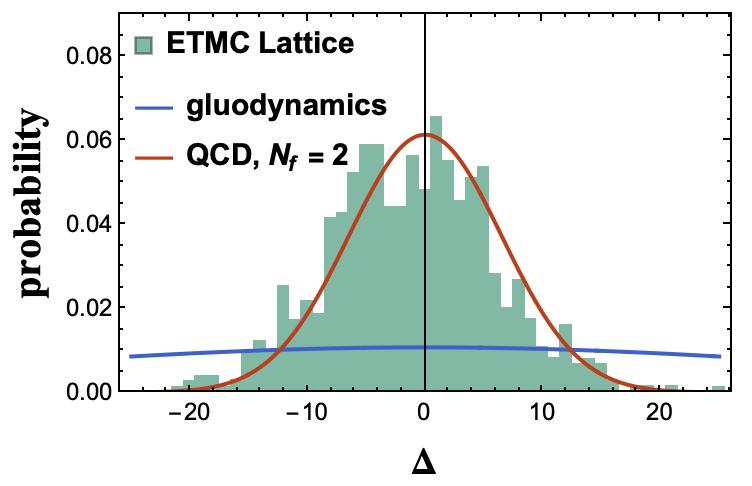
which is large. However, in QCD it is substantially screened by the light quarks, as illustrated in Fig. 1 with current quark mass MeV. The width of the distribution reads
| (10) |
Note that the topological susceptibility is sensitive to the determinantal mass . The details about how to fix the determinantal mass are given in Appendix C and in Liu et al. (2023a, 2024) (and references therein).
In Fig. 1 we show the unquenched ILM results (10) (red-solid) and quenched ILM (9) (blue-solid), compared to the lattice results from the ETMC collaboration Alexandrou et al. (2021). The latters used twisted mass clover-improved fermions , in a 4-volume with lattice spacing fm, and physical pion mass MeV. For the ILM parameters see below.
III Nucleon EM form factors
At finite vacuum angle , the QCD action in Euclidean signature is supplemented by the topological term
which is at the origin of strong CP violation. In the ILM, this contribution acts as a topological chemical potential for , by enhancing instantons and depleting anti-instantons. This affects most observables, and in particular the electromagnetic (EM) form factors of hadrons, as we will detail in this section.
The coupling to photon can be described by Dirac , Pauli , electric dipole moment form factor , and axial tensor form factor .
| (11) | ||||
with the Sachs FFs
| (12) |
and the electric dipole and axial-tensor FFs
| (13) |
with the two latters vanishing for . The magnetic and electric dipole moment are defined respectively,
| (14) |
For finite theta, (LABEL:EM_form) will be organized through
| (15) |
III.1 Emergent EM vertex
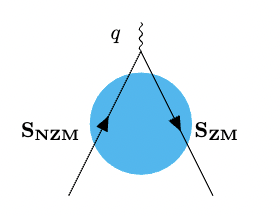
To see how the pseudoparticles contribute to the EM FF of hadrons, consider the instanton (antiinstanton) insertion to the charge current on a quark line illustrated in Fig. 2. In an instanton (antiinstanton) the incoming left-handed (right-handed) quark flips to a right-handed (left-handed) through a zero mode, then scatters off a virtual photon before exiting through a non-zero mode, with the result for a single quark Kochelev (2003). The effective interaction amplitude is defined as
| (16) | ||||
For a single instanton, the zero mode propagator is
| (17) |
with the zero modes defined in (37). The singular in the single instanton approximation is shifted to finite by disordering in the ILM Pobylitsa (1989); Schäfer and Shuryak (1998); Liu (2025) (and references therein). The determinantal mass is seen to follow from the constituent mass through a similar disordering Liu et al. (2024)
| (18) |
with the identification
The norm uses the zero mode profile defined as
| (20) |
The typical value of the constituent mass is about MeV Liu et al. (2023a, b); Liu (2025).
Inserting (17) into (16) yield the instanton induced effective EM vertex
| (21) | ||||
The effective vertex for the anti-instanton follows by interchanging , , and . Now the effective quark operator can be written as
| (22) |
The on-shell reduction of the in-out quark lines can be obtained by using the large time asymptotics as detailed in appendix B.2. More specifically, the on-shell reduction of the emergent vertex is ()
| (23) |
with the result for the Pauli contribution
| (24) | |||||
where is the modified Bessel function of the second kind.
III.2 -quark EDM
At zero vacuum angle, the Pauli contribution to the charge form factor in (15), receives a large contribution from pseudoparticles in the QCD instanton vacuum Kochelev (2003). We now show that this observation carries to the CP-odd contributions at finite vacuum angle. The Pauli part of the form factor of a quark of flavor is then
| (25) |
with the pseudoparticle induced form factor
| (26) |
The first parenthesis is identical to the Kochelev’s computation using an on-shell limit Kochelev (2003). The additional contribution in our case stems from use of the large Euclidean time approximation in the on-shell reduction scheme discussed in Appendix B. The latter is more appropriate for Euclidean formulations Liu and Zahed (2021).
The averaging of (25) over is carried using the grand-canonical ensemble detailed in appendix D, with the result
| (27) |
where we have used
It approaches to the asymptotic form in the large momentum transfer limit . Here is the vacuum connected topological susceptibility (10). A comparison of (26) to (LABEL:EM_form) yields the pseudoparticle contribution to the -quark form factors
| (28) |
in leading order in the density. Note that our result for the CP even form factor is different from the one in Kochelev (2003) which is IR singular. The reason is that our use of the large time asymptotic method presented in appendix B.2 is more appropriate for the on-shell reduction in Euclidean space as emphasized in Liu and Zahed (2021). The logarithmic sensitivity of the CP even form factor, will be fixed by the magnetic moment (see below).
III.3 Proton and neutron EDM
In the ILM, the proton and neutron are strongly correlated quark-diquark states, with a tight scalar-iso-scalar diquark and weaker axial-vector flavor-triplet diquark Schäfer and Shuryak (1998). This strong correlation in the scalar channel follows from the particle-anti-particle symmetry between the spin-0 pion and the spin-0 diquark. To take advantage of this observation, the proton and neutron SU(6) wavefunctions can be repacked in quark-diquark contributions Anselmino et al. (1993) (and references therein)
| (30) |
with the upper labels referring to the vector helicities. We can use (III.3) to evaluate the individual flavor contributions to the CP-odd contribution to the Pauli form factor. For that we note in the ILM the non-zero mode insertion can only happen on the unpaired quark, as the paired quarks in a diquark are locked by zero modes only.
Alternatively, we may use (29) to derive the CP-odd contribution in a proton and neutron through the Pauli form factor, hence
| (31) |
Using the empirical values efm and efm Patrignani et al. (2016), the electric dipole moments read
| (32) |
with a fixed ratio . The comparison to the recently reported lattice results and chiral perturbation calculation (ChPT) for the nucleon EDM are given in Table 1, with , and . Overall, our results appear to be in the range of some of the proton and neutron EDM reported by some lattice collaborations. For completeness, we note an earlier estimate of the neutron dipole moment using a numerical ensemble of pseudo-particles to describe the ILM, with a moment approximation to extract the EDM Faccioli et al. (2004).
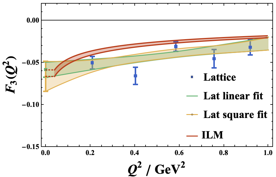
In Fig. 3 we show our result for the C-odd neutron electric dipole form factor (solid-red band) at low . The logarithmic infrared sensitivity of the induced pseudo-particle form factor in (26), is cutoff around fm-1 GeV (constant red dashed line) as we start to probe multi-pseudoparticle correlations, well beyond our current single instanton approach in the dilute ILM description. The momentum dependence is compared to the reported lattice C-odd electric dipole form factor (blue data) from the QCD lattice collaboration Liang et al. (2023). The green band is their estimated extrapolation using linear fits, and the yellow band is their estimated extrapolation using a square fit with additional term. The lattice simulations are carried out using overlap fermions, in a 4-volume ensemble with a lattice spacing .
IV Conclusions
In QCD, the breaking of conformal symmetry puts stringent constraints on the bulk hadronic correlations in the form of low energy theorems Novikov et al. (1981). These constraints are enforced in the QCD instanton vacuum in the form of stronger than Poisson fluctuations in the number of pseudoparticles, with a vacuum compressibility indicative of a quantum liquid. The fluctuations in the difference of the pseudoparticles are peaked around neutral topological charge with the variance, which is fixed by the topological susceptibility which is large in gluodynamics, but substantially screened in QCD. These are essential features of the ILM.
In the ILM, the Pauli form factor of constituent quarks receive a large contribution in the ILM, correcting an early observation in Kochelev (2003). In the presence of a CP violation by a small vacuum angle , we have shown that an axial contribution develops in the Pauli form factor, driven mostly by the vacuum topological susceptibility. We have used this result to estimate the induced the electric dipole moment in both the proton and neutron, as well as the semi-hard momentum dependence of the Pauli form factors , induced by the pseudoparticles. Our results are in the range of recently reported lattice results extrapolated at the physical pion mass Liang et al. (2023).
Acknowledgements
We thank Fangcheng He for some discussions. This work is supported by the Office of Science, U.S. Department of Energy under Contract No. DE-FG-88ER40388. This research is also supported in part within the framework of the Quark-Gluon Tomography (QGT) Topical Collaboration, under contract no. DE-SC0023646.
Appendix A Quark propagator in the single instanton background
In singular gauge, the instanton gauge field is given by
| (33) |
Here the instanton moduli is captured by the rigid color rotation , instanton location and size , with the singular gauge potential
| (34) |
The rigid color rotation
is defined with as an matrix with Pauli matrices embedded in the upper left corner. For the anti-instanton field, we substitute by and flip the sign in front of Levi-Cevita tensor, .
The effects of the quark masses on the quark propagator in the instanton or antiinstanton fields, are not known in closed form Liu and Zahed (2021). However, for small masses, the propagator can be expanded around the chiral limit
| (35) | ||||
The zero mode propagator reads
| (36) |
where the left-handed zero mode in singular gauge is
| (37) |
with , a color-spin locked 4-spinor.
The non-zero mode propagator in the chiral-split form reads Brown et al. (1978)
| (38) | ||||
where . The massless scalar propagator in the single instanton background field is defined as Brown et al. (1978)
| (39) |
The location of the instanton is set to be zero for simplicity and can be recovered by translational symmetry and . After a few steps of algebraic calculation, and can be recast in the form Schäfer and Shuryak (1998); Zubkov et al. (1999); Liu and Zahed (2021)
| (40) | ||||
and
| (41) | ||||
Note that the propagator for the anti-instanton can be obtained via the substitutions , and .
Appendix B Reduction scheme
The on-shell reduction of the Euclidean and massless quark propagator in the instanton background is subtle. In principle, it can be achieved in two ways: 1/ through LSZ reduction in the zero momentum limit; 2/ through the long term ”time” asymptotic. Here we will quote both procedures, although the long time asymptotics is the one that turns out to be IR free in most cases Liu and Zahed (2021) .
B.1 Zero Euclidean momentum
For massless quarks, the LSZ reduction in the zero momentum () limit reads
| (42) |
| (43) |
In the asymptotic limit , the reduction yields an on-shell free quark.
B.2 Large Euclidean time
The alternative reduction scheme that proves to be IR safe in most cases, consists in taking the large Euclidean ”time” asymptotics, to put the quark on mass shell, a common procedure on the lattice. More specifically, we have
| (44) | ||||
| (45) | ||||
where we have used the fact that
and
Combined with the reduction scheme in large Euclidean time, (23) reads
| (46) | ||||
Appendix C Determinantal mass in the instanton liquid
In the instanton liquid model, the concept of a determinantal mass characterises the width of the zero-mode zone, a key characteristic of the spontaneous breaking of chiral symmetry. It is sampled by the ensemble average of the fermionic determinant
| (47) |
a measure of the unquenching of the gauge configurations. In particular, a reduction in the density of pseudoparticles at low resolution
| (48) |
where denotes the quenched instanton size distribution in (3), and is the determinantal mass. Numerical simulations of ensembles of interacting pseudoparticles give Faccioli and Shuryak (2001)
In the thermodynamic limit ( with fixed) alongside the large limit, the emergent instantonic vertices exponentiate, giving
| (49) |
where the effective Lagrangian in Euclidean space reads Liu et al. (2024)
| (50) |
where the vertices are defined as
| (51) |
The emergent parameters and are fixed by the saddle point approximation. The effective coupling
| (52) |
is tied to the mean instanton size , density , and determinantal mass Schäfer and Shuryak (1996); Faccioli and Shuryak (2001); Shuryak and Zahed (2023); Liu et al. (2024) The screened topological charge is
| (53) |
In the saddle point approximation, the momentum dependent constituent mass is
| (54) |
along with the gap equation which naturally determines the determinantal mass Liu et al. (2024)
| (55) |
where the instanton-quark form factor is defined as
| (56) |
Using the instanton parameters fm-4, fm and the current mass MeV, the determinantal mass is
| (57) |
with the constituent mass of MeV Liu et al. (2023a, b); Liu (2025), and a quark condensate . The estimated determinantal mass is much closer to the numerical value of MeV Faccioli and Shuryak (2001).
Appendix D Averaging in grand canonical instanton liquid ensemble
Here we briefly outline the averaging over the fluctuations in the number of pseudoparticles in the ILM. In a grand canonical description where are allowed to fluctuate, the partition function of the QCD vacuum with finite vacuum angle is written as
| (58) | ||||
This partition function yield the distribution with the measures (6) and (8) at and or equivalently written as Diakonov et al. (1996); Schäfer and Shuryak (1998); Zahed (2021)
| (59) |
with mean and . As a result, vacuum expectation values of most quarks and gluon operators are averaged through
| (60) |
The averaging is carried out over the configurations with fixed (canonical ensemble average), followed by an ensemble averaging over the distribution (8).
Similarly, the evaluation of the hadronic matrix elements can be formulated as a large- reduction of a 3-point function
| (61) |
where is a pertinent source for the hadronic state .
Now with this grand canonical framework, the insertion of the gluonic scalar operator and topological charge operator in the the connected correlation function can be carried out by
| (62) |
| (63) |
The quark contribution are usually penalized by -counting, as they are rooted in the quark-instanton interaction. Therefore, in this case, the leading contribution will come from the fluctuations.
This approach can used to calculate the neutron EDM.
| (64) | ||||
In the book-keeping, the dominant contributions to neutron EDM are given by
| (65) |
References
- Sakharov (1967) A. D. Sakharov, Pisma Zh. Eksp. Teor. Fiz. 5, 32 (1967).
- Kharzeev et al. (2020) D. Kharzeev, E. Shuryak, and I. Zahed, Phys. Rev. D 102, 073003 (2020), arXiv:1906.04080 [hep-ph] .
- Diakonov et al. (1996) D. Diakonov, M. V. Polyakov, and C. Weiss, Nucl. Phys. B 461, 539 (1996), arXiv:hep-ph/9510232 .
- Schäfer and Shuryak (1998) T. Schäfer and E. V. Shuryak, Rev. Mod. Phys. 70, 323 (1998), arXiv:hep-ph/9610451 .
- Nowak et al. (1996) M. A. Nowak, M. Rho, and I. Zahed, Chiral nuclear dynamics (1996).
- Liu (2025) W.-Y. Liu, (2025), arXiv:2501.07776 [hep-ph] .
- Abel et al. (2020) C. Abel et al., Phys. Rev. Lett. 124, 081803 (2020), arXiv:2001.11966 [hep-ex] .
- Syritsyn et al. (2019) S. Syritsyn, T. Izubuchi, and H. Ohki, PoS Confinement2018, 194 (2019), arXiv:1901.05455 [hep-lat] .
- Alexandrou et al. (2021) C. Alexandrou, A. Athenodorou, K. Hadjiyiannakou, and A. Todaro, Phys. Rev. D 103, 054501 (2021), arXiv:2011.01084 [hep-lat] .
- Liang et al. (2023) J. Liang, A. Alexandru, T. Draper, K.-F. Liu, B. Wang, G. Wang, and Y.-B. Yang (QCD), Phys. Rev. D 108, 094512 (2023), arXiv:2301.04331 [hep-lat] .
- Leinweber (1999) D. B. Leinweber, in Workshop on Light-Cone QCD and Nonperturbative Hadron Physics (1999) pp. 138–143, arXiv:hep-lat/0004025 .
- Michael and Spencer (1995a) C. Michael and P. S. Spencer, Nucl. Phys. B Proc. Suppl. 42, 261 (1995a), arXiv:hep-lat/9411015 .
- Michael and Spencer (1995b) C. Michael and P. S. Spencer, Phys. Rev. D 52, 4691 (1995b), arXiv:hep-lat/9503018 .
- Biddle et al. (2018) J. C. Biddle, W. Kamleh, and D. B. Leinweber, PoS LATTICE2018, 256 (2018), arXiv:1903.07767 [hep-lat] .
- Athenodorou et al. (2018) A. Athenodorou, P. Boucaud, F. De Soto, J. Rodríguez-Quintero, and S. Zafeiropoulos, JHEP 02, 140 (2018), arXiv:1801.10155 [hep-lat] .
- Ringwald and Schrempp (1999) A. Ringwald and F. Schrempp, Phys. Lett. B 459, 249 (1999), arXiv:hep-lat/9903039 .
- Shuryak (1982) E. V. Shuryak, Nucl. Phys. B 203, 93 (1982).
- Diakonov (1996) D. Diakonov, Proc. Int. Sch. Phys. Fermi 130, 397 (1996), arXiv:hep-ph/9602375 .
- Shuryak (1999) E. V. Shuryak, (1999), arXiv:hep-ph/9909458 .
- Novikov et al. (1981) V. A. Novikov, M. A. Shifman, A. I. Vainshtein, and V. I. Zakharov, Nucl. Phys. B 191, 301 (1981).
- Liu et al. (2023a) W.-Y. Liu, E. Shuryak, and I. Zahed, (2023a), arXiv:2307.16302 [hep-ph] .
- Liu et al. (2024) W.-Y. Liu, E. Shuryak, and I. Zahed, (2024), arXiv:2404.03047 [hep-ph] .
- Kochelev (2003) N. I. Kochelev, Phys. Lett. B 565, 131 (2003), arXiv:hep-ph/0304171 .
- Pobylitsa (1989) P. V. Pobylitsa, Physics Letters B 226, 387 (1989).
- Liu et al. (2023b) W.-Y. Liu, E. Shuryak, and I. Zahed, Phys. Rev. D 107, 094024 (2023b), arXiv:2302.03759 [hep-ph] .
- Liu and Zahed (2021) Y. Liu and I. Zahed, (2021), arXiv:2102.07248 [hep-ph] .
- Faccioli et al. (2004) P. Faccioli, D. Guadagnoli, and S. Simula, Phys. Rev. D 70, 074017 (2004), arXiv:hep-ph/0406336 .
- Mereghetti et al. (2011) E. Mereghetti, J. de Vries, W. H. Hockings, C. M. Maekawa, and U. van Kolck, Phys. Lett. B 696, 97 (2011), arXiv:1010.4078 [hep-ph] .
- Bhattacharya et al. (2021) T. Bhattacharya, V. Cirigliano, R. Gupta, E. Mereghetti, and B. Yoon, Phys. Rev. D 103, 114507 (2021), arXiv:2101.07230 [hep-lat] .
- Dragos et al. (2021) J. Dragos, T. Luu, A. Shindler, J. de Vries, and A. Yousif, Phys. Rev. C 103, 015202 (2021), arXiv:1902.03254 [hep-lat] .
- Anselmino et al. (1993) M. Anselmino, E. Predazzi, S. Ekelin, S. Fredriksson, and D. B. Lichtenberg, Rev. Mod. Phys. 65, 1199 (1993).
- Patrignani et al. (2016) C. Patrignani et al. (Particle Data Group), Chin. Phys. C 40, 100001 (2016).
- Brown et al. (1978) L. S. Brown, R. D. Carlitz, D. B. Creamer, and C. Lee, Phys. Rev. D 17, 1583 (1978).
- Zubkov et al. (1999) A. G. Zubkov, O. V. Dubasov, and B. O. Kerbikov, Int. J. Mod. Phys. A 14, 241 (1999), arXiv:hep-ph/9712549 .
- Faccioli and Shuryak (2001) P. Faccioli and E. V. Shuryak, Phys. Rev. D 64, 114020 (2001), arXiv:hep-ph/0106019 .
- Schäfer and Shuryak (1996) T. Schäfer and E. V. Shuryak, Phys. Rev. D 53, 6522 (1996), arXiv:hep-ph/9509337 .
- Shuryak and Zahed (2023) E. Shuryak and I. Zahed, Phys. Rev. D 107, 034023 (2023), arXiv:2110.15927 [hep-ph] .
- Zahed (2021) I. Zahed, Phys. Rev. D 104, 054031 (2021), arXiv:2102.08191 [hep-ph] .