Present address: ]Oslo University Hospital, NO-0424 Oslo, Norway Present address: ]Department of Physics, University of Liverpool, L69 7ZE, United Kingdom Present address: ]Departamento de Estructura de la Materia, Física Térmica y Electrónica and IPARCOS, Universidad Complutense de Madrid, E-28040 Madrid, Spain Present address: ]Department of Physics, University of Johannesburg, P.O. Box 524, Auckland Park 2006, South Africa Present address: ]Department of Physics, University of Johannesburg, P.O. Box 524, Auckland Park 2006, South Africa Present address: ]Department of Physics, University of Liverpool, L69 7ZE, United Kingdom
The ISOLDE Collaboration
Nuclear Level Density and -ray Strength Function of and the impact on the -process
Abstract
Proton- coincidences from reactions between a beam and a deuterated polyethylene target have been analyzed with the inverse-Oslo method to find the nuclear level density (NLD) and -ray strength function (SF) of . The capture cross section has been calculated using the Hauser-Feshbach model in TALYS using the measured NLD and SF as constraints. The results confirm that the reaction acts as a bottleneck when relying on one-zone nucleosynthesis calculations. However, the impact of this reaction is strongly dampened in multi-zone models of low-metallicity AGB stars experiencing i-process nucleosynthesis.
I Introduction
The origin and production mechanism of the heavy elements has been under investigation for a long time. The first direct observations of nucleosynthesis of heavy elements was reported by P. Merrill in 1952 [1]. Soon after, the mechanism behind the production of heavy elements through neutron capture was outlined in the famous B2FH paper in 1957 [2].
Nucleosynthesis beyond the Fe/Ni mass region is due to the slow neutron capture (s-process), rapid neutron capture (r-process), photo-disintegration processes, and more recent results call for an intermediate neutron capture process (i-process) [3, 4]. These processes are sensitive to nuclear properties such as the nuclear level densities (NLD) and -ray strength functions (SF). The availability and uncertainties in nuclear data affect the ability to reliably calculate reaction rates, in particular for the r- and i-processes as they involve neutron-rich nuclei for which data is non-existing or at the very least sparse. This can have significant impact on the neutron capture rates and on the final abundance distribution of elements and their isotopes predicted by models. Currently, the vast majority of nuclei for which NLDs and SFs have been measured lie at, or very near, the line of stability [5]. Experimentally measured NLD and SF can provide significant constraints on calculated neutron capture rates which are relevant for nucleosynthesis models [6, 7].
Away from stability, directly measured cross sections are not available and NLDs and SFs can provide the necessary constraints. The Oslo method is particularly suitable as it extracts NLD and SF simultaneously [8, 9]. These quantities, together with the optical model potentials, are the main ingredients of the Hauser-Feshbach theory [10] to calculate neutron capture cross-sections and reaction rates. The Oslo Method has been extended to include total absorption spectroscopy following -decay leading to the -Oslo method [11] and has demonstrated the versatility of the Oslo method and its applicability even for nuclei far from stability [11, 12, 13, 14, 15]. The -Oslo method requires specific -Q value conditions for the mother-daughter pair placing a limit on the nuclei which can be measured with this technique.
Another approach is to use inverse kinematics with radioactive beams. Here, the beam intensity is the main limiting factor. Applying the Oslo method to experimental data from an inverse kinematics experiment was first demonstrated in Ref. [16] extracting the NLD and SF of following a pick-up reaction. In this paper, we have applied this inverse-Oslo method to data from a radioactive ion beam experiment to extract the NLD and SF of . Based on these results, the neutron capture rate of was constrained using the Hauser-Feshbach theory, which is of particular importance for our understanding of the weak i-process. In the weak i-process the neutron density is large (), but exposure is low due to a quick and abrupt termination of the neutron production. In such a case only the first n-capture peak elements are produced significantly [17]. This was studied in Ref. [17], where it was found that the reaction have a major impact on the overall production rate of heavier elements, essentially acting as a bottleneck for the entire weak i-process. Constraining the reaction could improve our understanding of the i-process nucleosynthesis.

II Experiment and analysis
The experiment was performed using the HIE-ISOLDE facility at CERN [18], where 1.4 GeV proton beam from the PSBooster bombarded a uranium carbide target inducing fission. The evaporated fission products were ionized by the resonance ionization laser ion source (RILIS) [19] and the ions were separated by the General Purpose Separator (GPS) to be collected and cooled by a penning trap (REXTRAP) [20]. The ions were then charge bread to a charge state by an electron-beam ion source (REXEBIS) [21, 22]. The highly ionized ions were re-accelerated by the HIE-ISOLDE linear accelerator to an energy of 4.47(1) MeV/u. The pps intense beam impinged on a g/cm2 thick secondary deuterated polyethylene target (99% enrichment in deuterium) [23] placed at the Miniball experimental station and produced the desired reactions. The total time of beam on target was approximately hours. The same reaction has previously been measured at ISOLDE by Ref. [24], but at a much lower beam energy of MeV/u. That data-set was not considered as it only reached excitation energies up to 3.5 MeV, much less than what is required for the Oslo Method.
Protons from the reaction were measured with the C-REX particle detector array [25, 26], while coincident -rays were measured using the Miniball detector array [27, 28]. Only the downstream particle array was considered due to low yields in the upstream array. The particle detectors considered covered angles between and in the laboratory frame (CM angles to ). Two of the eight Miniball high-purity germanium (HPGe) clusters [28] were replaced by six large-volume ( inch) LaBr3:Ce detectors to increase the high -ray energy efficiency of the array. The placement of each detector is given in table 1. Signals from the C-REX detectors were processed by an analog data acquisition system (DAQ) which fed four 32-channel analogue-to-digital converter (ADC) modules from Mesytec. The signals from the -ray detectors were processed by a digital DAQ consisting of XIA Digital Gamma Finders (DGF-4C). The two systems were synchronized, read out simultaneously, and the data written to disk.
| Detector | Target distance | ||
|---|---|---|---|
| [deg] | [deg] | [cm] | |
| LaBr3:Ce 1 | 136 | 147 | 25 |
| LaBr3:Ce 2 | 184 | 147 | 25 |
| LaBr3:Ce 3 | 210 | 147 | 25 |
| LaBr3:Ce 4 | 32 | 64 | 25 |
| LaBr3:Ce 5 | 358 | 64 | 25 |
| LaBr3:Ce 6 | 330 | 64 | 25 |
| Miniball 1 | 148 | 64 | 12 |
| Miniball 2 | 228 | 64 | 12 |
| Miniball 3 | 188 | 101 | 12 |
| Miniball 4 | 358 | 101 | 12 |
| Miniball 5 | 312 | 56 | 12 |
| Miniball 6 | 32 | 56 | 12 |
Prompt particle- coincidences were selected from the data by applying time gates on the time difference between the detected -rays and particles, while the reaction was selected by applying the appropriate energy cut on the matrix. Background events were selected in a similar fashion by placing time gates of half the size as the prompt gate on either sides of the prompt peak. This resulted in a total of and background subtracted proton- coincidences with the LaBr3:Ce detectors and the Miniball clusters, respectively. The low number of proton- coincidences with the LaBr3:Ce compared to those with the Miniball detectors is due to the lower geometric efficiency of the LaBr3:Ce detectors which were located considerably further from the target. Despite having only a quarter of the Miniball coincidences, the more efficient LaBr3:Ce detectors measured the majority of high-energy -ray transitions. For this reason, the results presented here are based on the analysis of proton- coincident events from the LaBr3:Ce detectors only.
Due to the considerable residual kinetic energy of the -ray energies were Doppler corrected. The maximum deflection of the residual was less than and the maximum spread in velocity was less than %. The correction was performed using a constant factor based only on the -detector angle relative to the beam axis.
For each proton- event the excitation energy was calculated from the kinematic reconstruction of the two-body reaction. The proton- coincidences were collected in an excitation- energy matrix shown in Fig. 1(a). Due to the Lorentz boost associated with inverse-kinematics there were no well-resolved levels in the particle spectra suitable for an in-beam calibration and the FWHM of the excitation energy was MeV.
The first step to obtain NLDs and SFs from excitation- matrices is to correct for the detector response using the unfolding method [29] by using a detector response deduced from a Geant4 [30] simulation of the experimental setup [31]. This resulted in the unfolded matrix shown in Fig. 1(b).
Next, an iterative subtraction method [32] is applied to the unfolded matrix in order to deduce the distribution of primary -rays emitted from each excitation bin, resulting in the first generation matrix shown in Fig. 1(c).
The first-generation matrix is proportional to the -ray transmission coefficients and the NLD at the final excitation energy following the first decay of the cascade [8]
| (1) |
The NLD and transmission coefficients are extracted by normalizing the first-generation -ray spectra for each excitation bin and by fitting the experimental matrix () with a theoretical matrix [8]
| (2) |
by minimizing
| (3) |
where and are treated as free parameters for each -ray energy and final energy , respectively. The denominator, , represents the experimental uncertainty in the first-generation matrix. Considering the experimental resolution and to ensure that only primary transitions, originating in the quasi-continuum, are considered a minimum -ray energy of MeV was selected. Similarly, only excitation energy bins between and MeV were included in the fit. These and energy regions have been chosen based on the guidelines of Ref. [33].
The resulting -ray transmission coefficients are converted to SF by
under the assumption that the transmission coefficients are dominated by dipole transitions.
The theoretical first-generation matrix, (2), is invariant under transformation of NLD and SF [8]
| (4) |
where , and are transformation parameters. This means that the extracted NLD and SF do not represent the physical NLD and SF, but contain information on the functional shape. To deduce the absolute values of the NLD and SF the extracted NLD and SF will have to be normalized to auxiliary data.
III Normalization of NLD and SF
Many nuclei along the island of stability have auxiliary data available with which the normalization of the NLDs and SFs is achieved. Typical data used for this purpose are the level density from resolved discrete states, the level density at the neutron separation energy ( MeV) from s- and/or p-wave neutron resonance spacing data, and the average radiative widths of s-wave neutron resonances. When applying the Oslo method, NLDs do not extend to as the method probes the NLD at the final excitation energy , the maximum energy possible to be considered in the first-generation matrix is , and is typically the neutron separation energy (depending on reaction kinematics) [33], but in this case slightly below at MeV, which corresponds to a final and highest excitation energy of 4.1 MeV. Hence, the measured NLDs are typically interpolated to the NLDs from resonance data at .
The impact on the uncertainty of NLDs and SF on the availability of neutron resonance data has recently been demonstrated [34]. In the absence of neutron resonance data, the resonance spacing or radiative widths of neutron resonances are generally estimated from systematics of neighboring nuclei, see for instance Refs.[35, 36, 37]. Similarly, for -Oslo measurements various combinations of solutions have been used ranging from systematic information of nearby nuclei [11, 38], model calculations [14, 39, 38], or the Shape method [39, 38, 40, 41]. Neither for nor for surrounding nuclei are neutron resonance data available. The situation is further aggravated by an incomplete level scheme at low excitation energies resulting in an unreliable level density of resolved discrete states which, together with the low experimental resolution, makes the application of the Shape method not ideal. With the absence of any reliable normalization points the only practical solution for normalizing the NLD and SF is the reliance on model estimates.
III.1 Bayesian analysis
Despite the lack of auxiliary data for normalization it is still possible to constrain the experimental NLD and SF as the true values are expected to fall within the range of commonly accepted models. For example, the NLD in statistical nuclei grows exponentially and are often well reproduced by large shell model calculations [42, 12] at low energies and the constant temperature [43], Back-shifted Fermi Gas [44] or microscopic Hartree-Fock [45] calculations at high energies. Similarly, the SF is expected to follow the tail of the GDR and typically features resonances such as the upbend and/or a PDR. This is typically well described by the phenomenological Simple Modified Lorentzian model (SMLO) or the microscopic mean field plus quasi-particle random phase approximation both of which being the recommended global models to describe the PSF [5]. By assuming a combination of NLD and SF models one can constrain the possible values for the normalization parameters, , and in Eq. (4).
This can be taken a step further by considering several models for NLD and SF to get a range of acceptable normalization parameters. To perform such an analysis we apply Bayesian statistics. Analyzing Oslo method data within a Bayesian statistics framework has previously been demonstrated by Midtbø et al. [9] and our analysis is based on the framework presented therein. The starting point of the normalization analysis is Bayes’ theorem
| (5) |
where is the posterior probability of a set of normalization and model parameters , given a set of non-normalized measured NLD points and SF points . The likelihood is the probability of measuring non-normalized NLD and SF given the set of parameters . is the prior probability of a set of normalization and model parameters. The prior will be further discussed in section III.3, while the physical models and their parameters are presented in section III.2 and summarized in table 2. The evidence is the probability of measuring the non-normalized NLD and SF, and can be treated as a normalization factor. With the assumption of Gaussian distributed uncertainties of the measured non-normalized NLD and SF leads to the likelihood
| (6) |
with corresponding to
| (7) | ||||
| (8) | ||||
| (9) | ||||
| (10) | ||||
| (11) | ||||
Here, represents the likelihood of measuring a set of NLDs given the known level density from discrete levels , is the likelihood given a specific NLD model and is the likelihood given a SF model. The NLD between excitation energies between and MeV are considered in Eq. (7) while NLD between and MeV are considered in Eq. (8). All measured SF energies are included in Eq. (9). The likelihood is included to further constrain the SF using the measured SF in as the SF above the neutron separation energy are typically very similar in neighboring nuclei. , () and () are the normalized NLD (SF) and standard deviation, given a set of normalization parameters , respectively (see Eq. 4).
III.2 Models
A total of three NLD models and four SF models have been considered, making the total number of inferred posteriors twelve. In this section we will describe the models considered.
NLD
For energies above the point where the model space of the shell model calculation is exhausted the NLD has been modeled with three different models. These include the Back-Shifted Fermi Gas (BSFG) model [51, 52]
| (12) |
where is the level density parameter, is the energy shift and is the spin-cutoff parameter. The Constant Temperature (CT) model [53]
| (13) |
where is the nuclear temperature and is an energy shift parameter. Lastly, tabulated Hartree-Fock-Bogoliubov (HFB) calculations [54] were also considered, and allowed to be re-normalized through
| (14) |
where again is used to denote an energy shift, is a slope parameter and are the tabulated NLDs. It should be noted that in eqs. (12), (13), and (14) are not the same parameters and will be sub-scripted whenever there is ambiguity which parameter is being referenced. The spin distribution for the BSFG and CT models was given by the Bethe/Ericson distribution [51, 53]
| (15) |
with the spin-cutoff parameterized by [55, 56]
| (16) |
where is the discrete spin-cutoff parameter, obtained from shell-model result as discussed in section III.3, with a constant spin distribution at energies below MeV.
SF
For the SF we have considered the Simplified version of the Modified Lorentzian model (SMLO) [57] and the microscopic Gogny-HFB plus quasi-particle random phase approximation (Gogny-HFB+QRPA) with phenomenological corrections [58], which are the recommended global models for the SF [5]. The SMLO model describes the E1 SF with the giant dipole resonance (GDR) for photo-emission strength and is given by
| (17) |
where is the centroid of the GDR, is the Thomas-Reiche-Kuhn sum rule [57] and is the temperature at the final excitation energy. The width,
| (18) |
depends on the final temperature and the which is the width found in the photo-absorption strength function. Within the SMLO model the M1 strength is parameterized as two standard Lorentzians (SLO)
| (19) |
for the scissors and the spin-flip resonances. The low-energy upbend is modeled as a simple exponential [54]. From the shape of the non-normalized SF there are no obvious signs of a scissors resonance which is consistent with the relatively low estimated axial deformation of [59] and has been omitted from further consideration in the model for the SF. The assumed M1 strength contributions are thus
| (20) |
where is the mean energy, is the width and the cross-section of the spin-flip resonance. The parameters of the upbend, and have no physical interpretation and are treated as free parameters chosen to best describe the shape of the upbend. The assumption for the M1 multipolarity of the upbend is based on results from shell model calculations [60, 61, 42, 62] and from a measurement albeit not conclusively [63].
In the Gogny-HFB+QRPA model, the photo-emission E1 strength is given by
| (21) |
where is the strength found in Gogny-HFB+QRPA calculations. The phenomenological parameters , are free parameters and is the excitation energy of the initial level. The strength is allowed to be scaled and shifted through the free parameters and , respectively. The M1 strength was estimated within the SMLO model, Eq. (20).
Data points from a Coulomb dissociation measurement of are also considered [64]. This features a strong narrow Pygmy dipole resonance (PDR) at MeV which has been accounted for by including a SLO in the E1 strength. Since the extracted SF in only extends to MeV we cannot determine if such a PDR also exists in . In order to account for either possibility, we have repeated the analysis both with and without including the PDR, observed in , in the strength. In the latter case, the two experimental points at MeV and MeV of were excluded and removed from consideration in Eq. (11). A list of all model combinations and their parameters are listed in table 2.
III.3 Parameter priors
For all model parameters, the probability distribution were assumed to be Gaussian or truncated Gaussian probability density functions (PDF). The latter used for parameters where there are physical justifications for why the values cannot have certain values (e.g. no negative temperature).
The normalization parameters required to transform the NLD and SF to the physical solution are arbitrary and we have no a priori knowledge other than that and has to be positive. Ideally, flat prior probability distributions should be used for , and , with the former two truncated to positive values. However, this is computationally expensive. Instead truncated Gaussian distributions were used for and and a Gaussian probability distribution for . To maintain an un-informed prior the standard deviation of the probability distribution for and were set to times the centroid, while the standard deviation of the prior probability distribution of was set to 1/MeV. The latter was chosen due to the high sensitivity of the likelihood to this parameter. The centroid of the prior probability distributions were selected to be the , and values that maximized the likelihood Eq. (6). Numerical values for the centroids of , and PDFs are listed in Appendix A.
| Model | Parameters | |
|---|---|---|
| CT | , , , | |
| BSFG | , , , | |
| HFB | , | |
| SMLO (E1) | , , | |
| HFB-QRPA (E1) | , , , , | |
| PDR (E1) | , , | |
| M1 | , , , , |
For the NLD models fairly weak informed priors were used. In the case of the BSFG model the level density parameter mean value of MeV was selected as the approximate mean of the systematics from Refs. [52, 65], Refs. [66, 67] and Ref. [67] with width . The shift parameter is a Gaussian with MeV and MeV. Similarly the CT model priors were selected from the systematics of Ref. [67] with widths of MeV for the temperature and MeV for the shift parameter . The slope and shift parameters and for the HFB was centered around MeV-1/2 and MeV with widths of MeV-1/2 and MeV, respectively. The discrete spin-cutoff parameter from eq. 16 was found to be by examining the tabulated shell model levels while the spin-cutoff at the neutron separation energy is from an average of spin-cut off models in [54, 52, 66]. In both cases an uncertainty of was assumed. The priors for all NLD model parameters are listed in Table 3.
| Parameter | |||
|---|---|---|---|
| MeV | MeV | ||
| (BSFG) | MeV | MeV | |
| MeV | MeV | ||
| (CT) | MeV | MeV | |
| (HFB) | MeV-1/2 | MeV-1/2 | |
| (HFB) | MeV | MeV | |
The parameters for the SMLO model were taken from the systematics in [57]. Unless an uncertainty was provided it was assumed to be . The scale and shift for the Gogny-HFB+QRPA was assumed to be centered around and MeV, respectively, with a width of MeV for both. The phenomenological parameters and are taken from [58], while the probability distribution of the initial excitation energy was modeled as a truncated Gaussian at the excitation range used to extract the NLD and SF ( and MeV) with a mean of MeV and a standard deviation of MeV. The spin-flip and upbend parameters were taken from [57] assuming uncertainty, except for , where the width was assumed to be the same as the mean. Lastly, the PDR parameters were taken from [64]. All priors parameters related to the SF models are listed in Table 4.
| Parameter | |||
|---|---|---|---|
| MeV | MeV | ||
| MeV | MeV | ||
| mb | mb | ||
| MeV | MeV | ||
| MeV-4 | MeV-4 | ||
| MeV | MeV | ||
| MeV | MeV | ||
| MeV | MeV | ||
| MeV | |||
| mb | mb | ||
| MeV | MeV | ||
| MeV | MeV | ||
| mb | mb | ||
| MeV-3 | MeV-3 | ||
| 1/MeV | 1/MeV |
III.4 Hauser-Feshbach calculations and results
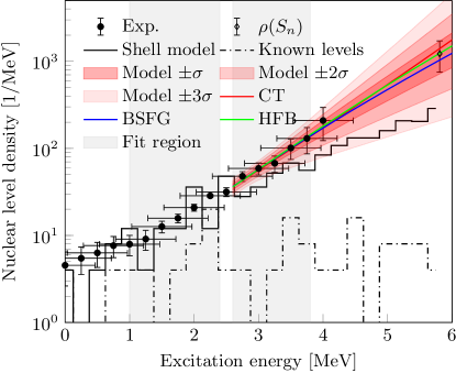
For each sample the normalized NLD and SF are calculated and the marginal posterior probability distribution for each NLD and SF point is obtained for each combination of NLD and SF models. Weighting each combination of models equally, the average normalized NLD and SF are shown in Fig. 2 and 3, respectively. The , and credibility intervals (1, 2 and 3 standard deviations) of the model predictions are found by calculating the NLD and SF for each sample and weighting each combination of models equally. The posterior mean values for all model and normalization parameters are listed in Appendix A. The impact of including the PDR structure in the models for the SF reported by [64] is shown in Fig. 4 to be negligible for the normalization of the SF. The NLD at the neutron separation energy is found to be MeV-1 by averaging the NLD models.


The measured NLD and SF in were used in Hauser-Feshbach calculations to constrain the neutron capture cross section of . From each posterior sample of normalization and model parameters tabulated NLD and SF values were generated from linear interpolation and used as input to the TALYS111Version 1.96 reaction code [70]. Since the level scheme of is far from complete only the first two discrete levels were included in the Hauser-Feshbach calculations, while above those the provided tabulated NLD was used. Each realization of the capture cross section and reaction rate is weighted equally to obtain a mean cross section and reaction rate and the credibility bands shown in Figs. 5 and 6. The impact of the optical model potential (OMP) has been tested by performing calculations with the phenomenological OMP of Ref. [71] and the microscopic OMP of Ref. [72] and found to have a negligible contribution to the uncertainty.


In the sensitivity study of Ref. [17] the reaction rates were taken from the JINA REACLIB v1.1 library [76], indicated by the red dashed line in Fig. 6. The maximum and minimum reaction rates considered by Ref. [17] are based on the models listed in Table 1 of Ref. [78], and these results have been reproduced as indicated by the red band in Fig. 5 and 6. For comparison, the capture cross section and rate with the default selection of NLD (CT+Fermi-Gas), SF (SMLO [57]+LEE) models, and optical model potential (local phenomenological OMP) in TALYS version 1.96 are shown by the black dashed lines in Figs. 5 and 6.
IV Discussion
The Oslo method relies on external nuclear data for the normalization. In the absence of those, additional uncertainties may be induced and model dependencies may become significant. This is apparent through the relatively large uncertainties toward on the measured NLD for .
The challenge specific to inverse kinematic reactions is the Lorentz boost which causes a strong angular dependence in the kinematic reconstruction of the residual excitation energy. This leads to an excitation-energy resolution which is limited by the angular opening of the particle telescope’s active areas. The consequences are most apparent in the NLD where very little structures are visible.
In contrast, the measured SF still retains noticeable features and clearly exhibits a well established enhancement for MeV similar to those found in other isotopes [79, 80, 34, 44, 81, 12]. Its observation indicates that the upbend is a structure which exists also away from stability. The upbend in is predicted to be due to M1 strength, based on large-scale shell model calculations [46], and shown by the black solid line in Fig. 3. The significant strength in the enhancement and the simultaneous absence of a measurable scissors resonance may be supportive of the suggested connection of the two structures [82, 61], although results on the SF in seem to contradict this [83].
The calculated capture cross section in Fig. 5 features an uncertainty of , constraining the cross section considerably. It is interesting to note that our cross section, lies consistently higher than the recommended values as provided in TALYS and TENDL but is smaller than those of JEFF 3.3 for keV. These differences highlight the necessity for measurements of NLDs and SFs, especially for nuclei away from stability.
Ref. [17] allows the capture rate to vary within the red band as indicated in Fig. 6, with the nominal value taken from the JINA REACLIB v1.1 database [76]. Our results constrain the capture rate significantly and show that this rate is found at the high end of the range used by Ref. [17]. This suggests a short exposure time for the weak i-process and could help pinpoint details in the stellar environment responsible to produce neutrons.
V Astrophysical implications


The capture rate was suggested to be of key importance for the overall production of heavy elements during the i-process nucleosynthesis taking place in Sakurai’s object or rapidly accreting white dwarfs [17]. One possible astrophysical site with similar i-process conditions are low-metallicity low-mass stars during the early thermally pulsating Asymptotic Giant Branch (AGB) phase [84, 85, 86, 87, 88]. During this stage, protons can be engulfed by the convective thermal pulse. As they are transported downward by convection on a timescale of about 1 hr, they are burnt rapidly by . After the decay of to in about 10 min, the reaction is activated at the bottom of the thermal pulse and leads to neutron densities of up to cm-3. Stellar modeling was performed with the stellar evolution code STAREVOL [89, 90, 91]. A 1 AGB model at a metallicity of [Fe/H] is considered. This model is discussed in detail in Ref. [88].
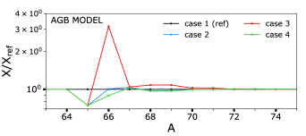
We estimated the impact of the new rate on the i-process nucleosynthesis in these objects. The effects are evaluated on both multi-zone stellar evolution models and in one-zone nucleosynthesis calculations. We used a reaction network including 1160 nuclei, linked through 2123 nuclear reactions (-, -, -captures and -decays) and weak interactions (electron captures, -decays). Nuclear reaction rates were taken from BRUSLIB, the Nuclear Astrophysics Library of the Université Libre de Bruxelles222Available at http://www.astro.ulb.ac.be/bruslib/ [77] and the updated experimental and theoretical rates from the NETGEN interface [92]. Additional details can be found in Refs. [88, 93, 94]. In our sensitivity analysis, eight cases were investigated. We consider, for the reaction, the recommended Maxwellian-averaged cross section (MACS) from this work ( mb at 30 keV) as well as the minimum (1 mb at 30 keV) and maximum (19 mb at 30 keV) rates predicted by a global unconstrained TALYS calculation (i.e. maximum and minimum reaction rates as prescribed in Ref. [17]). Additionally, the rate of was also varied because has a half-life of hr (55 hr for ), which is fast enough to partially bypass the neutron capture during the i-process. For , we considered the minimum (10 mb at 30 keV) and maximum (70 mb at 30 keV) MACS predicted by TALYS for different NLD and SF models. We also considered the uncertainties related to the nominal MACS evaluated in this study by varying it by mb at 30 keV (cases 1B, 1C, 2B and 2C). The different cases considered are reported in Table 5.
| 65Ni() | 66Ni() | |
|---|---|---|
| case 1 | TALYS min | nominal |
| case 1B | TALYS min | nominal mb |
| case 1C | TALYS min | nominal mb |
| case 2 | TALYS max | nominal |
| case 2B | TALYS max | nominal mb |
| case 2C | TALYS max | nominal mb |
| case 3 | TALYS max | TALYS min |
| case 4 | TALYS max | TALYS max |
The initial abundances of the one-zone model correspond to the chemical composition in the thermal pulse of the AGB stellar model, just before the start of the proton ingestion event. The temperature and density were fixed to 220 MK and 2500 g cm-3, respectively, which are typical values in the pulse of low-metallicity AGB models. The nucleosynthesis was calculated over a total time of s ( days). To mimic the proton ingestion episode in the one-zone model, an initial abundance of protons was set to and leading to maximum neutron densities of cm-3 and cm-3, respectively. For a low initial proton abundance, a weak i-process develops and elements up to the first peak () are synthesized (Fig. 7, black pattern). With more protons, a larger neutron density is reached and elements of the third peak (Fig. 7, red pattern) are produced. For this particular case, the final chemical composition is found to be very similar to that of the full multi-zone AGB model where densities up to cm-3 are reached.
As shown in Fig. 8, increasing the rate of (case 2) leads to a smaller production of (as a result of decay) by a factor of in both weak and strong i-process cases. Lowering (case 3) has the strongest impact since now acts as a bottleneck. In the weak i-process case (Fig. 8, top panel), it leads to an overproduction of by a factor of to the detriment of isotopes (), which are underproduced by a factor of at maximum. For a higher neutron density (Fig. 8, bottom panel), the production of isotopes () is enhanced by a factor of typically . The uncertainties on the nominal MACS obtained in this work ( mb at 30 keV) induce a variation of about a factor of at (dashed lines in Fig. 8, top panel).
Ref. [17] investigated the case of a weak i-process using one-zone models with an initial metallicity of [Fe/H] ([Fe/H] here) and different reaction rates (most of () rates coming from the JINA REACLIB library [76]). Although the physical inputs are different, in the case of a weak i-process the results are qualitatively similar to those of Ref. [17]: an underproduction of the elements with when adopting a low rate.
However, when considering a full multi-zone AGB calculation, the impact of is strongly dampened (Fig. 9). The overproduction of in case 3 is clearly present but the enrichment is a factor of lower. In the stellar model, multiple zones with different temperatures, densities, chemical compositions and irradiations are mixed together by convection leading to a dilute production of the elements, an effect that cannot be captured by one-zone calculations.
The impact of the reaction appears to be marginal in low-metallicity AGB stars experiencing i-process nucleosynthesis. It shows that one-zone calculations are inherently approximate and cannot guarantee to reproduce the accurate physics picture for a system. We should also emphasize that only one i-process site was investigated and we cannot exclude a different impact of in other sites such as e.g. rapidly accreting white dwarfs [95].
VI Summary
In this paper we have presented experimental NLD and SF of the unstable nucleus. It is the first time the Oslo method has been applied to an inverse kinematics experiment with a radioactive beam. Due to the lack of reliable nuclear data for the NLD and SF are normalized to model predictions resulting in relatively large uncertainties. Hauser-Feshbach calculations were performed with the extracted NLD and SF to find the neutron capture cross section of . The result of these calculations showed a rather high capture rate compared to the theoretical range, and can help improve our understanding of the i-process nucleosynthesis. In agreement with Ref. [17], we find that the reaction acts as a bottleneck when using one-zone models. Nevertheless, the impact is strongly dampened in multi-zone low-metallicity AGB stellar models experiencing i-process nucleosynthesis. This reaction may however have a different impact in other i-process sites.
Acknowledgements.
The authors would like to thank the accelerator team at CERN ISOLDE for providing excellent running conditions. This study has been funded by the Research Council of Norway through its grants to the Norwegian Nuclear Research Centre (Project No. 341985) and the Norwegian Centre for CERN-related Research (Project No. 310713). Additional research project grants were provided by the Research Council of Norway (Grants No. 263030, 325714 and 245882), the National Research Foundation of South Africa (Grant No. 118846), the EU Horizon 2020 research and innovation program through ENSAR2 (Grant No. 654002), and the U.S. Department of Energy, Office of Science, Office of Nuclear Physics under Contract No. DE-AC02-05CH11231 (LBNL) and Contract No. DE-AC52-07NA27344 (LLNL). Funding was also provided by the German BMBF under contracts 05P18PKCIA, 05P21PKCI1, 05P15RDCIA, and ‘Verbundprojekt’ 05P18PKCI1, 05P18PKCI1. This work was supported by the Fonds de la Recherche Scientifique-FNRS under Grant No IISN 4.4502.19. L.S. and S.G. are senior FRS-F.N.R.S. research associates and A.C. is a post-doctorate FRS-F.N.R.S. fellow. G.R. acknowledges the support by the Bulgarian Ministry of Education and Science within the National Roadmap for Research Infrastructures (object CERN). Additional support was provided by the Research Foundation Flanders (FWO, Belgium) under GOA/2015/010 (BOF KU Leuven) and the FWO and F.R.S.-FNRS under the Excellence of Science (EOS) programme (No. 40007501).Appendix A Prior and posterior parameters
| Models | A (MeV-1) | B (MeV-3) | (MeV-1) |
|---|---|---|---|
| CT+SMLO+M1 | 1.863 | 0.538 | -0.037 |
| CT+SMLO+PDR+M1 | 1.745 | 0.484 | -0.00453 |
| CT+QRPA+M1 | 2.378 | 0.677 | -0.141 |
| CT+QRPA+PDR+M1 | 2.152 | 0.574 | -0.111 |
| BSFG+SMLO+M1 | 2.033 | 0.670 | -0.0781 |
| BSFG+SMLO+PDR+M1 | 1.826 | 0.520 | -0.0177 |
| BSFG+QRPA+M1 | 2.652 | 0.882 | -0.120 |
| BSFG+QRPA+PDR+M1 | 2.034 | 0.541 | -0.0709 |
| HFB+SMLO+M1 | 1.916 | 0.620 | -0.0446 |
| HFB+SMLO+PDR+M1 | 1.880 | 0.580 | -0.0327 |
| HFB+QRPA+M1 | 2.270 | 0.528 | -0.122 |
| HFB+QRPA+PDR+M1 | 2.169 | 0.557 | -0.102 |
| Parameter | Value |
|---|---|
| MeV-1 | |
| MeV-3 | |
| MeV-1 | |
| MeV | |
| MeV | |
| MeV | |
| MeV | |
| mb | |
| MeV | |
| MeV | |
| mb | |
| MeV-3 | |
| MeV-1 |
| Parameter | Value |
|---|---|
| MeV-1 | |
| MeV-3 | |
| MeV-1 | |
| MeV | |
| MeV | |
| MeV | |
| MeV | |
| mb | |
| MeV | |
| MeV | |
| mb | |
| MeV | |
| MeV | |
| mb | |
| MeV-3 | |
| MeV-1 |
| Parameter | Value |
|---|---|
| MeV-1 | |
| MeV-3 | |
| MeV-1 | |
| MeV | |
| MeV | |
| MeV | |
| MeV-4 | |
| MeV | |
| MeV | |
| MeV | |
| MeV | |
| mb | |
| MeV-3 | |
| MeV-1 |
| Parameter | Value |
|---|---|
| MeV-1 | |
| MeV-3 | |
| MeV-1 | |
| MeV | |
| MeV | |
| MeV | |
| MeV-4 | |
| MeV | |
| MeV | |
| MeV | |
| MeV | |
| mb | |
| MeV | |
| MeV | |
| mb | |
| MeV-3 | |
| MeV-1 |
| Parameter | Value |
|---|---|
| MeV-1 | |
| MeV-3 | |
| MeV-1 | |
| MeV | |
| MeV | |
| MeV | |
| MeV | |
| mb | |
| MeV | |
| MeV | |
| mb | |
| MeV-3 | |
| MeV-1 |
| Parameter | Value |
|---|---|
| MeV-1 | |
| MeV-3 | |
| MeV-1 | |
| MeV | |
| MeV | |
| MeV | |
| MeV | |
| mb | |
| MeV | |
| MeV | |
| mb | |
| MeV | |
| MeV | |
| mb | |
| MeV-3 | |
| MeV-1 |
| Parameter | Value |
|---|---|
| MeV-1 | |
| MeV-3 | |
| MeV-1 | |
| MeV | |
| MeV | |
| MeV | |
| MeV-4 | |
| MeV | |
| MeV | |
| MeV | |
| MeV | |
| mb | |
| MeV-3 | |
| MeV-1 |
| Parameter | Value |
|---|---|
| MeV-1 | |
| MeV-3 | |
| MeV-1 | |
| MeV | |
| MeV | |
| MeV | |
| MeV-4 | |
| MeV | |
| MeV | |
| MeV | |
| MeV | |
| mb | |
| MeV | |
| MeV | |
| mb | |
| MeV-3 | |
| MeV-1 |
| Parameter | Value |
|---|---|
| MeV-1 | |
| MeV-3 | |
| MeV-1 | |
| MeV-1/2 | |
| MeV | |
| MeV | |
| MeV | |
| mb | |
| MeV | |
| MeV | |
| mb | |
| MeV-3 | |
| MeV-1 |
| Parameter | Value |
|---|---|
| MeV-1 | |
| MeV-3 | |
| MeV-1 | |
| MeV-1/2 | |
| MeV | |
| MeV | |
| MeV | |
| mb | |
| MeV | |
| MeV | |
| mb | |
| MeV | |
| MeV | |
| mb | |
| MeV-3 | |
| MeV-1 |
| Parameter | Value |
|---|---|
| MeV-1 | |
| MeV-3 | |
| MeV-1 | |
| MeV-1/2 | |
| MeV | |
| MeV | |
| MeV-4 | |
| MeV | |
| MeV | |
| MeV | |
| MeV | |
| mb | |
| MeV-3 | |
| MeV-1 |
| Parameter | Value |
|---|---|
| MeV-1 | |
| MeV-3 | |
| MeV-1 | |
| MeV-1/2 | |
| MeV | |
| MeV | |
| MeV-4 | |
| MeV | |
| MeV | |
| MeV | |
| MeV | |
| mb | |
| MeV | |
| MeV | |
| mb | |
| MeV-3 | |
| MeV-1 |
References
- Merrill [1952] P. Merrill, Technetium in the stars, Science 115, 479 (1952).
- Burbidge et al. [1957] E. M. Burbidge, G. R. Burbidge, W. A. Fowler, and F. Hoyle, Synthesis of the elements in stars, Reviews of Modern Physics 29, 547 (1957).
- Cowan and Rose [1977] J. J. Cowan and W. K. Rose, Production of C-14 and neutrons in red giants, The Astrophysical Journal 212, 149 (1977).
- Roederer et al. [2016] I. U. Roederer, A. I. Karakas, M. Pignatari, and F. Herwig, The Diverse Origines of Neutron-capture Elements in The Metal-poor Star HD 94028: Possible Detection of Products of i-process Nucleosynthesis, The Astrophysical Journal 821, 37 (2016).
- Goriely et al. [2019] S. Goriely, P. Dimitriou, M. Wiedeking, T. Belgya, R. Firestone, J. Kopecky, M. Krtička, V. Plujko, R. Schwengner, S. Siem, H. Utsunomiya, S. Hilaire, S. Péru, Y. S. Cho, D. M. Filipescu, N. Iwamoto, T. Kawano, V. Varlamov, and R. Xu, Reference database for photon strength functions, European Physical Journal A 55, 172 (2019).
- Larsen et al. [2019] A. C. Larsen, A. Spyrou, S. N. Liddick, and M. Guttormsen, Novel techniques for constraining neutron-capture rates relevant for r-process heavy-element nucleosynthesis (2019).
- Wiedeking and Goriely [2024] M. Wiedeking and S. Goriely, Phil. Trans. R. Soc. A. 382, 20230125 (2024).
- Schiller et al. [2000] A. Schiller, L. Bergholt, M. Guttormsen, E. Melby, J. Rekstad, and S. Siem, Extraction of level density and strength function from primary spectra, Nuclear Instruments and Methods in Physics Research, Section A: Accelerators, Spectrometers, Detectors and Associated Equipment 447, 498 (2000).
- Midtbø et al. [2021] J. E. Midtbø, F. Zeiser, E. Lima, A. C. Larsen, G. M. Tveten, M. Guttormsen, F. L. Bello Garrote, A. Kvellestad, and T. Renstrøm, A new software implementation of the Oslo method with rigorous statistical uncertainty propagation, Computer Physics Communications 262, 10.1016/j.cpc.2020.107795 (2021).
- Hauser and Feshbach [1952] W. Hauser and H. Feshbach, The Inelastic Scattering of Neutrons, Phys. Rev. 87, 366 (1952).
- Spyrou et al. [2014] A. Spyrou, S. N. Liddick, A. C. Larsen, M. Guttormsen, K. Cooper, A. C. Dombos, D. J. Morrissey, F. Naqvi, G. Perdikakis, S. J. Quinn, T. Renstrøm, J. A. Rodriguez, A. Simon, C. S. Sumithrarachchi, and R. G. T. Zegers, Novel technique for constraining r -process (n, ) reaction rates, Physical Review Letters 113, 232502 (2014).
- Larsen et al. [2018] A. C. Larsen, J. E. Midtbø, M. Guttormsen, T. Renstrøm, S. N. Liddick, A. Spyrou, S. Karampagia, B. A. Brown, O. Achakovskiy, S. Kamerdzhiev, D. L. Bleuel, A. Couture, L. C. Campo, B. P. Crider, A. C. Dombos, R. Lewis, S. Mosby, F. Naqvi, G. Perdikakis, C. J. Prokop, S. J. Quinn, and S. Siem, Enhanced low-energy -decay strength of 70Ni and its robustness within the shell model, Physical Review C 97, 054329 (2018).
- Lewis et al. [2019] R. Lewis, S. N. Liddick, A. C. Larsen, A. Spyrou, D. L. Bleuel, A. Couture, L. C. Campo, B. P. Crider, A. C. Dombos, M. Guttormsen, S. Mosby, F. Naqvi, G. Perdikakis, C. J. Prokop, S. J. Quinn, T. Renstrøm, and S. Siem, Experimental constraints on the reaction rate, Physical Review C 99, 034601 (2019).
- Liddick et al. [2016] S. N. Liddick, A. Spyrou, B. P. Crider, F. Naqvi, A. C. Larsen, M. Guttormsen, M. Mumpower, R. Surman, G. Perdikakis, D. L. Bleuel, A. Couture, L. Crespo Campo, A. C. Dombos, R. Lewis, S. Mosby, S. Nikas, C. J. Prokop, T. Renstrom, B. Rubio, S. Siem, and S. J. Quinn, Experimental Neutron Capture Rate Constraint Far from Stability, Physical Review Letters 116, 242502 (2016).
- Liddick et al. [2019] S. N. Liddick, A. C. Larsen, M. Guttormsen, A. Spyrou, B. P. Crider, F. Naqvi, J. E. Midtbø, F. L. Bello Garrote, D. L. Bleuel, L. Crespo Campo, A. Couture, A. C. Dombos, F. Giacoppo, A. Görgen, K. Hadynska-Klek, T. W. Hagen, V. W. Ingeberg, B. V. Kheswa, R. Lewis, S. Mosby, G. Perdikakis, C. J. Prokop, S. J. Quinn, T. Renstrøm, S. J. Rose, E. Sahin, S. Siem, G. M. Tveten, M. Wiedeking, and F. Zeiser, Benchmarking the extraction of statistical neutron capture cross sections on short-lived nuclei for applications using the -oslo method, Phys. Rev. C 100, 024624 (2019).
- Ingeberg et al. [2020] V. W. Ingeberg, S. Siem, M. Wiedeking, K. Sieja, D. L. Bleuel, C. P. Brits, T. D. Bucher, T. S. Dinoko, J. L. Easton, A. Görgen, M. Guttormsen, P. Jones, B. V. Kheswa, N. A. Khumalo, A. C. Larsen, E. A. Lawrie, J. J. Lawrie, S. N. Majola, K. L. Malatji, L. Makhathini, B. Maqabuka, D. Negi, S. P. Noncolela, P. Papka, E. Sahin, R. Schwengner, G. M. Tveten, F. Zeiser, and B. R. Zikhali, First application of the Oslo method in inverse kinematics, European Physical Journal A 56, 68 (2020).
- McKay et al. [2020] J. E. McKay, P. A. Denissenkov, F. Herwig, G. Perdikakis, and H. Schatz, The impact of (n,) reaction rate uncertainties on the predicted abundances of i-process elements with 32 Z 48 in the metal-poor star HD94028, Monthly Notices of the Royal Astronomical Society 491, 5179 (2020).
- Kadi et al. [2018] Y. Kadi, M. A. Fraser, and A. Papageorgiou-Koufidou, HIE-ISOLDE: technical design report for the energy upgrade, edited by Y. Kadi (CERN, Geneva, 2018).
- Fedoseyev et al. [2000] V. N. Fedoseyev, G. Huber, U. Köster, J. Lettry, V. I. Mishin, H. Ravn, and V. Sebastian, The ISOLDE laser ion source for exotic nuclei, Hyperfine Interactions 127, 409 (2000).
- Ames et al. [2005] F. Ames, G. Bollen, P. Delahaye, O. Forstner, G. Huber, O. Kester, K. Reisinger, and P. Schmidt, Cooling of radioactive ions with the Penning trap REXTRAP, Nuclear Instruments and Methods in Physics Research, Section A: Accelerators, Spectrometers, Detectors and Associated Equipment 538, 17 (2005).
- Wenander [2002] F. Wenander, EBIS as charge breeder for radioactive ion beam accelerators, Nuclear Physics A 701, 528 (2002).
- Wenander [2010] F. Wenander, Charge breeding of radioactive ions with EBIS and EBIT, Journal of Instrumentation 5 (10), C10004.
- Kheswa et al. [2020] N. Kheswa, T. Dinoko, and M. Wiedeking, The production of deuterated polyethylene targets, EPJ Web of Conferences 229, 03003 (2020).
- Diriken et al. [2014] J. Diriken, N. Patronis, A. Andreyev, S. Antalic, V. Bildstein, A. Blazhev, I. Darby, H. De Witte, J. Eberth, J. Elseviers, V. Fedosseev, F. Flavigny, C. Fransen, G. Georgiev, R. Gernhauser, H. Hess, M. Huyse, J. Jolie, T. Kröll, R. Krücken, R. Lutter, B. Marsh, T. Mertzimekis, D. Muecher, F. Nowacki, R. Orlandi, A. Pakou, R. Raabe, G. Randisi, P. Reiter, T. Roger, M. Seidlitz, M. Seliverstov, K. Sieja, C. Sotty, H. Tornqvist, J. Van De Walle, P. Van Duppen, D. Voulot, N. Warr, F. Wenander, and K. Wimmer, Study of the deformation-driving d5/2 orbital in using one-neutron transfer reactions, Physics Letters B 736, 533 (2014).
- Hellgartner et al. [2023] S. Hellgartner, D. Mücher, K. Wimmer, V. Bildstein, J. Egido, R. Gernhäuser, R. Krücken, A. Nowak, M. Zielińska, C. Bauer, M. Benito, S. Bottoni, H. De Witte, J. Elseviers, D. Fedorov, F. Flavigny, A. Illana, M. Klintefjord, T. Kröll, R. Lutter, B. Marsh, R. Orlandi, J. Pakarinen, R. Raabe, E. Rapisarda, S. Reichert, P. Reiter, M. Scheck, M. Seidlitz, B. Siebeck, E. Siesling, T. Steinbach, T. Stora, M. Vermeulen, D. Voulot, N. Warr, and F. Wenander, Axial and triaxial degrees of freedom in 72Zn, Physics Letters B 841, 137933 (2023).
- Hellgartner [2015] S. C. Hellgartner, Probing Nuclear Shell Structure beyond the N= 40 Subshell using Multiple Coulomb Excitation and Transfer Experiments, Ph.D. thesis, Technische Universität München, Lehrstuhl E12 für Experimentalphysik (2015).
- Eberth et al. [2001] J. Eberth, G. Pascovici, H. G. Thomas, N. Warr, D. Weisshaar, D. Habs, P. Reiter, P. Thirolf, D. Schwalm, C. Gund, H. Scheit, M. Lauer, P. Van Duppen, S. Franchoo, M. Huyse, R. M. Lieder, W. Gast, J. Gerl, and K. P. Lieb, MINIBALL A Ge detector array for radioactive ion beam facilities, Progress in Particle and Nuclear Physics 46, 389 (2001).
- Warr et al. [2013] N. Warr, J. Van de Walle, M. Albers, F. Ames, B. Bastin, C. Bauer, V. Bildstein, A. Blazhev, S. Bönig, N. Bree, B. Bruyneel, P. A. Butler, J. Cederkäll, E. Clément, T. E. Cocolios, T. Davinson, H. De Witte, P. Delahaye, D. D. DiJulio, J. Diriken, J. Eberth, A. Ekström, J. Elseviers, S. Emhofer, D. V. Fedorov, V. N. Fedosseev, S. Franchoo, C. Fransen, L. P. Gaffney, J. Gerl, G. Georgiev, R. Gernhäuser, T. Grahn, D. Habs, H. Hess, A. M. Hurst, M. Huyse, O. Ivanov, J. Iwanicki, D. G. Jenkins, J. Jolie, N. Kesteloot, O. Kester, U. Köster, M. Krauth, T. Kröll, R. Krücken, M. Lauer, J. Leske, K. P. Lieb, R. Lutter, L. Maier, B. A. Marsh, D. Mücher, M. Münch, O. Niedermaier, J. Pakarinen, M. Pantea, G. Pascovici, N. Patronis, D. Pauwels, A. Petts, N. Pietralla, R. Raabe, E. Rapisarda, P. Reiter, A. Richter, O. Schaile, M. Scheck, H. Scheit, G. Schrieder, D. Schwalm, M. Seidlitz, M. Seliverstov, T. Sieber, H. Simon, K. H. Speidel, C. Stahl, I. Stefanescu, P. G. Thirolf, H. G. Thomas, M. Thürauf, P. Van Duppen, D. Voulot, R. Wadsworth, G. Walter, D. Weißhaar, F. Wenander, A. Wiens, K. Wimmer, B. H. Wolf, P. J. Woods, K. Wrzosek-Lipska, and K. O. Zell, The Miniball spectrometer, The European Physical Journal A 49, 40 (2013).
- Guttormsen et al. [1996] M. Guttormsen, T. S. Tveter, L. Bergholt, F. Ingebretsen, and J. Rekstad, The unfolding of continuum -ray spectra, Nuclear Instruments and Methods in Physics Research, Section A: Accelerators, Spectrometers, Detectors and Associated Equipment 374, 371 (1996).
- Agostinelli et al. [2003] S. Agostinelli, J. Allison, K. Amako, J. Apostolakis, H. Araujo, P. Arce, M. Asai, D. Axen, S. Banerjee, G. Barrand, F. Behner, L. Bellagamba, J. Boudreau, L. Broglia, A. Brunengo, H. Burkhardt, S. Chauvie, J. Chuma, R. Chytracek, G. Cooperman, G. Cosmo, P. Degtyarenko, A. Dell’Acqua, G. Depaola, D. Dietrich, R. Enami, A. Feliciello, C. Ferguson, H. Fesefeldt, G. Folger, F. Foppiano, A. Forti, S. Garelli, S. Giani, R. Giannitrapani, D. Gibin, J. J. G. Cadenas, I. González, G. G. Abril, G. Greeniaus, W. Greiner, V. Grichine, A. Grossheim, S. Guatelli, P. Gumplinger, R. Hamatsu, K. Hashimoto, H. Hasui, A. Heikkinen, A. Howard, V. Ivanchenko, A. Johnson, F. W. Jones, J. Kallenbach, N. Kanaya, M. Kawabata, Y. Kawabata, M. Kawaguti, S. Kelner, P. Kent, A. Kimura, T. Kodama, R. Kokoulin, M. Kossov, H. Kurashige, E. Lamanna, T. Lampén, V. Lara, V. Lefebure, F. Lei, M. Liendl, W. Lockman, F. Longo, S. Magni, M. Maire, E. Medernach, K. Minamimoto, P. M. de Freitas, Y. Morita, K. Murakami, M. Nagamatu, R. Nartallo, P. Nieminen, T. Nishimura, K. Ohtsubo, M. Okamura, S. O’Neale, Y. Oohata, K. Paech, J. Perl, A. Pfeiffer, M. G. Pia, F. Ranjard, A. Rybin, S. Sadilov, E. D. Salvo, G. Santin, T. Sasaki, N. Savvas, Y. Sawada, S. Scherer, S. Sei, V. Sirotenko, D. Smith, N. Starkov, H. Stoecker, J. Sulkimo, M. Takahata, S. Tanaka, E. Tcherniaev, E. S. Tehrani, M. Tropeano, P. Truscott, H. Uno, L. Urban, P. Urban, M. Verderi, A. Walkden, W. Wander, H. Weber, J. P. Wellisch, T. Wenaus, D. C. Williams, D. Wright, T. Yamada, H. Yoshida, and D. Zschiesche, Geant4—a simulation toolkit, Nuclear Instruments and Methods in Physics Research Section A: Accelerators, Spectrometers, Detectors and Associated Equipment 506, 250 (2003).
- Ingeberg [2022] V. W. Ingeberg, vetlewi/MiniballREX: Ni67, https://github.com/vetlewi/MiniballREX (2022).
- Guttormsen et al. [1987] M. Guttormsen, T. Ramsøy, and J. Rekstad, The first generation of -rays from hot nuclei, Nuclear Inst. and Methods in Physics Research, A 255, 518 (1987).
- Larsen et al. [2011] A. C. Larsen, M. Guttormsen, M. Krtička, E. Běták, A. Bürger, A. Görgen, H. T. Nyhus, J. Rekstad, A. Schiller, S. Siem, H. K. Toft, G. M. Tveten, A. V. Voinov, and K. Wikan, Analysis of possible systematic errors in the oslo method, Physical Review C 83, 034315 (2011).
- Ingeberg et al. [2022] V. W. Ingeberg, P. Jones, L. Msebi, S. Siem, M. Wiedeking, A. A. Avaa, M. V. Chisapi, E. A. Lawrie, K. L. Malatji, L. Makhathini, S. P. Noncolela, and O. Shirinda, Nuclear level density and -ray strength function of , Physical Review C 106, 054315 (2022).
- Larsen et al. [2016] A. C. Larsen, M. Guttormsen, R. Schwengner, D. L. Bleuel, S. Goriely, S. Harissopulos, F. L. Bello Garrote, Y. Byun, T. K. Eriksen, F. Giacoppo, A. Görgen, T. W. Hagen, M. Klintefjord, T. Renstrøm, S. J. Rose, E. Sahin, S. Siem, T. G. Tornyi, G. M. Tveten, A. V. Voinov, and M. Wiedeking, Experimentally constrained and reaction rates relevant to -process nucleosynthesis, Physical Review C 93, 045810 (2016).
- Brits et al. [2019] C. P. Brits, K. L. Malatji, M. Wiedeking, B. V. Kheswa, S. Goriely, F. L. B. Garrote, D. L. Bleuel, F. Giacoppo, A. Görgen, M. Guttormsen, K. Hadynska-Klek, T. W. Hagen, S. Hilaire, V. W. Ingeberg, H. Jia, M. Klintefjord, A. C. Larsen, S. N. T. Majola, P. Papka, S. Péru, B. Qi, T. Renstrøm, S. J. Rose, E. Sahin, S. Siem, G. M. Tveten, and F. Zeiser, Nuclear level densities and -ray strength functions of , Phys. Rev. C 99, 054330 (2019).
- Kheswa et al. [2015] B. V. Kheswa, M. Wiedeking, F. Giacoppo, S. Goriely, M. Guttormsen, A. C. Larsen, F. L. Bello Garrote, T. K. Eriksen, A. Görgen, T. W. Hagen, P. E. Koehler, M. Klintefjord, H. T. Nyhus, P. Papka, T. Renstrøm, S. Rose, E. Sahin, S. Siem, and T. Tornyi, Galactic production of138La: Impact of138,139La statistical properties, Physics Letters, Section B: Nuclear, Elementary Particle and High-Energy Physics 744, 268 (2015).
- Sweet et al. [2024] A. Sweet, D. L. Bleuel, N. D. Scielzo, L. A. Bernstein, A. C. Dombos, B. L. Goldblum, C. M. Harris, T. A. Laplace, A. C. Larsen, R. Lewis, S. N. Liddick, S. M. Lyons, F. Naqvi, A. Palmisano-Kyle, A. L. Richard, M. K. Smith, A. Spyrou, J. Vujic, and M. Wiedeking, Nuclear level density and -decay strength of , Phys. Rev. C 109, 054305 (2024).
- Spyrou et al. [2024] A. Spyrou, D. Mücher, P. A. Denissenkov, F. Herwig, E. C. Good, G. Balk, H. C. Berg, D. L. Bleuel, J. A. Clark, C. Dembski, P. A. DeYoung, B. Greaves, M. Guttormsen, C. Harris, A. C. Larsen, S. N. Liddick, S. Lyons, M. Markova, M. J. Mogannam, S. Nikas, J. Owens-Fryar, A. Palmisano-Kyle, G. Perdikakis, F. Pogliano, M. Quintieri, A. L. Richard, D. Santiago-Gonzalez, G. Savard, M. K. Smith, A. Sweet, A. Tsantiri, and M. Wiedeking, First study of the reaction to constrain the conditions for the astrophysical process, Phys. Rev. Lett. 132, 202701 (2024).
- Mücher et al. [2023] D. Mücher, A. Spyrou, M. Wiedeking, M. Guttormsen, A. C. Larsen, F. Zeiser, C. Harris, A. L. Richard, M. K. Smith, A. Görgen, S. N. Liddick, S. Siem, H. C. Berg, J. A. Clark, P. A. DeYoung, A. C. Dombos, B. Greaves, L. Hicks, R. Kelmar, S. Lyons, J. Owens-Fryar, A. Palmisano, D. Santiago-Gonzalez, G. Savard, and W. W. von Seeger, Extracting model-independent nuclear level densities away from stability, Phys. Rev. C 107, L011602 (2023).
- Wiedeking et al. [2021] M. Wiedeking, M. Guttormsen, A. C. Larsen, F. Zeiser, A. Görgen, S. N. Liddick, D. Mücher, S. Siem, and A. Spyrou, Independent normalization for -ray strength functions: The shape method, Physical Review C 104, 014311 (2021).
- Brown and Larsen [2014] B. A. Brown and A. C. Larsen, Large low-energy M1 strength for Fe 56,57 within the nuclear shell model, Physical Review Letters 113, 252502 (2014).
- Guttormsen et al. [2015] M. Guttormsen, M. Aiche, F. L. Bello Garrote, L. A. Bernstein, D. L. Bleuel, Y. Byun, Q. Ducasse, T. K. Eriksen, F. Giacoppo, A. Görgen, F. Gunsing, T. W. Hagen, B. Jurado, M. Klintefjord, A. C. Larsen, L. Lebois, B. Leniau, H. T. Nyhus, T. Renstrøm, S. J. Rose, E. Sahin, S. Siem, T. G. Tornyi, G. M. Tveten, A. Voinov, M. Wiedeking, and J. Wilson, Experimental level densities of atomic nuclei, The European Physical Journal A 51, 170 (2015).
- Campo et al. [2017] L. C. Campo, A. C. Larsen, F. L. B. Garrote, T. K. Eriksen, F. Giacoppo, A. Görgen, M. Guttormsen, M. Klintefjord, T. Renstrøm, E. Sahin, S. Siem, T. G. Tornyi, and G. M. Tveten, Investigating the decay of 65Ni from particle- coincidence data, Physical Review C 96, 014312 (2017).
- Renstrøm et al. [2016] T. Renstrøm, H. T. Nyhus, H. Utsunomiya, R. Schwengner, S. Goriely, A. C. Larsen, D. M. Filipescu, I. Gheorghe, L. A. Bernstein, D. L. Bleuel, T. Glodariu, A. Görgen, M. Guttormsen, T. W. Hagen, B. V. Kheswa, Y. W. Lui, D. Negi, I. E. Ruud, T. Shima, S. Siem, K. Takahisa, O. Tesileanu, T. G. Tornyi, G. M. Tveten, and M. Wiedeking, Low-energy enhancement in the -ray strength functions of Ge 73,74, Physical Review C 93, 64302 (2016).
- Midtbø et al. [2018] J. E. Midtbø, A. C. Larsen, T. Renstrøm, F. L. Bello Garrote, and E. Lima, Consolidating the concept of low-energy magnetic dipole decay radiation, Physical Review C 98, 064321 (2018).
- Feroz and Hobson [2008] F. Feroz and M. P. Hobson, Multimodal nested sampling: an efficient and robust alternative to Markov Chain Monte Carlo methods for astronomical data analyses, Monthly Notices of the Royal Astronomical Society 384, 449 (2008).
- Feroz et al. [2009] F. Feroz, M. P. Hobson, and M. Bridges, MultiNest: an efficient and robust Bayesian inference tool for cosmology and particle physics, Monthly Notices of the Royal Astronomical Society 398, 1601 (2009).
- Feroz et al. [2019] F. Feroz, M. P. Hobson, E. Cameron, and A. N. Pettitt, Importance Nested Sampling and the MultiNest Algorithm, The Open Journal of Astrophysics 2, 10.21105/astro.1306.2144 (2019).
- Buchner et al. [2014] J. Buchner, A. Georgakakis, K. Nandra, L. Hsu, C. Rangel, M. Brightman, A. Merloni, M. Salvato, J. Donley, and D. Kocevski, X-ray spectral modelling of the AGN obscuring region in the CDFS: Bayesian model selection and catalogue, Astronomy & Astrophysics 564, A125 (2014).
- Bethe [1936] H. A. Bethe, An Attempt to Calculate the Number of Energy Levels of a Heavy Nucleus, Physical Review 50, 332 (1936).
- Gilbert and Cameron [1965] A. Gilbert and A. G. W. Cameron, a Composite Nuclear-Level Density Formula With Shell Corrections, Canadian Journal of Physics 43, 1446 (1965).
- Ericson [1959] T. Ericson, A statistical analysis of excited nuclear states, Nuclear Physics 11, 481 (1959).
- Goriely et al. [2008] S. Goriely, S. Hilaire, and A. J. Koning, Improved microscopic nuclear level densities within the Hartree-Fock-Bogoliubov plus combinatorial method, Physical Review C - Nuclear Physics 78, 064307 (2008).
- Capote et al. [2009] R. Capote, M. Herman, P. Obložinský, P. G. Young, S. Goriely, T. Belgya, A. V. Ignatyuk, A. J. Koning, S. Hilaire, V. A. Plujko, M. Avrigeanu, O. Bersillon, M. B. Chadwick, T. Fukahori, Z. Ge, Y. Han, S. Kailas, J. Kopecky, V. M. Maslov, G. Reffo, M. Sin, E. S. Soukhovitskii, and P. Talou, RIPL - Reference Input Parameter Library for Calculation of Nuclear Reactions and Nuclear Data Evaluations, Nuclear Data Sheets 110, 3107 (2009).
- Guttormsen et al. [2017] M. Guttormsen, S. Goriely, A. C. Larsen, A. Görgen, T. W. Hagen, T. Renstrøm, S. Siem, N. U. H. Syed, G. Tagliente, H. K. Toft, H. Utsunomiya, A. V. Voinov, and K. Wikan, Quasicontinuum decay of 91,92Zr: Benchmarking indirect (n,) cross section measurements for the s process, Physical Review C 96, 024313 (2017).
- Goriely and Plujko [2019] S. Goriely and V. Plujko, Simple empirical E1 and M1 strength functions for practical applications, Physical Review C 99, 014303 (2019).
- Goriely et al. [2018] S. Goriely, S. Hilaire, S. Péru, and K. Sieja, Gogny-HFB+QRPA dipole strength function and its application to radiative nucleon capture cross section, Physical Review C 98, 014327 (2018).
- Hilaire and Girod [2007] S. Hilaire and M. Girod, Large-scale mean-field calculations from proton to neutron drip lines using the D1S Gogny force, The European Physical Journal A 33, 237 (2007).
- Schwengner et al. [2013] R. Schwengner, S. Frauendorf, and A. C. Larsen, Low-Energy Enhancement of Magnetic Dipole Radiation, Physical Review Letters 111, 232504 (2013).
- Frauendorf and Schwengner [2022] S. Frauendorf and R. Schwengner, Evolution of low-lying M1 modes in germanium isotopes, Physical Review C 105, 034335 (2022).
- Sieja [2017] K. Sieja, Electric and Magnetic Dipole Strength at Low Energy, Phys. Rev. Lett. 119, 052502 (2017).
- Jones et al. [2018] M. D. Jones, A. O. Macchiavelli, M. Wiedeking, L. A. Bernstein, H. L. Crawford, C. M. Campbell, R. M. Clark, M. Cromaz, P. Fallon, I. Y. Lee, M. Salathe, A. Wiens, A. D. Ayangeakaa, D. L. Bleuel, S. Bottoni, M. P. Carpenter, H. M. Davids, J. Elson, A. Görgen, M. Guttormsen, R. V. F. Janssens, J. E. Kinnison, L. Kirsch, A. C. Larsen, T. Lauritsen, W. Reviol, D. G. Sarantites, S. Siem, A. V. Voinov, and S. Zhu, Examination of the low-energy enhancement of the -ray strength function of , Phys. Rev. C 97, 024327 (2018).
- Rossi et al. [2013] D. M. Rossi, P. Adrich, F. Aksouh, H. Alvarez-Pol, T. Aumann, J. Benlliure, M. Böhmer, K. Boretzky, E. Casarejos, M. Chartier, A. Chatillon, D. Cortina-Gil, U. Datta Pramanik, H. Emling, O. Ershova, B. Fernandez-Dominguez, H. Geissel, M. Gorska, M. Heil, H. T. Johansson, A. Junghans, A. Kelic-Heil, O. Kiselev, A. Klimkiewicz, J. V. Kratz, R. Krücken, N. Kurz, M. Labiche, T. Le Bleis, R. Lemmon, Y. A. Litvinov, K. Mahata, P. Maierbeck, A. Movsesyan, T. Nilsson, C. Nociforo, R. Palit, S. Paschalis, R. Plag, R. Reifarth, D. Savran, H. Scheit, H. Simon, K. Sümmerer, A. Wagner, W. Waluś, H. Weick, and M. Winkler, Measurement of the dipole polarizability of the unstable neutron-rich nucleus 68Ni, Physical Review Letters 111, 242503 (2013).
- Von Egidy et al. [1988] T. Von Egidy, H. H. Schmidt, and A. N. Behkami, Nuclear level densities and level spacing distributions: Part II, Nuclear Physics, Section A 481, 189 (1988).
- Egidy and Bucurescu [2005] T. v. Egidy and D. Bucurescu, Systematics of nuclear level density parameters, Physical Review C 72, 044311 (2005).
- von Egidy and Bucurescu [2009] T. von Egidy and D. Bucurescu, Experimental energy-dependent nuclear spin distributions, Physical Review C 80, 054310 (2009).
- Junde et al. [2005] H. Junde, H. Xiaolong, and J. K. Tuli, Nuclear Data Sheets for A = 67, Nuclear Data Sheets 106, 159 (2005).
- Diriken et al. [2015] J. Diriken, N. Patronis, A. Andreyev, S. Antalic, V. Bildstein, A. Blazhev, I. G. Darby, H. De Witte, J. Eberth, J. Elseviers, V. N. Fedosseev, F. Flavigny, C. Fransen, G. Georgiev, R. Gernhauser, H. Hess, M. Huyse, J. Jolie, T. Kröll, R. Krücken, R. Lutter, B. A. Marsh, T. Mertzimekis, D. Muecher, R. Orlandi, A. Pakou, R. Raabe, G. Randisi, P. Reiter, T. Roger, M. Seidlitz, M. Seliverstov, C. Sotty, H. Tornqvist, J. Van De Walle, P. Van Duppen, D. Voulot, N. Warr, F. Wenander, and K. Wimmer, Experimental study of the 66Ni(d,p)67Ni one-neutron transfer reaction, Physical Review C 91, 54321 (2015).
- Koning et al. [2007] A. J. Koning, S. Hilaire, and M. C. Duijvestijn, TALYS-1.0, in ND2007 (EDP Sciences, Les Ulis, France, 2007) pp. 211–214.
- Koning and Delaroche [2003] A. Koning and J. Delaroche, Local and global nucleon optical models from 1 to 200 , Nuclear Physics A 713, 231 (2003).
- Bauge et al. [2001] E. Bauge, J. P. Delaroche, and M. Girod, Lane-consistent, semimicroscopic nucleon-nucleus optical model, Phys. Rev. C 63, 024607 (2001).
- Plompen et al. [2020] A. J. M. Plompen, O. Cabellos, C. De Saint Jean, M. Fleming, A. Algora, M. Angelone, P. Archier, E. Bauge, O. Bersillon, A. Blokhin, F. Cantargi, A. Chebboubi, C. Diez, H. Duarte, E. Dupont, J. Dyrda, B. Erasmus, L. Fiorito, U. Fischer, D. Flammini, D. Foligno, M. R. Gilbert, J. R. Granada, W. Haeck, F.-J. Hambsch, P. Helgesson, S. Hilaire, I. Hill, M. Hursin, R. Ichou, R. Jacqmin, B. Jansky, C. Jouanne, M. A. Kellett, D. H. Kim, H. I. Kim, I. Kodeli, A. J. Koning, A. Y. Konobeyev, S. Kopecky, B. Kos, A. Krása, L. C. Leal, N. Leclaire, P. Leconte, Y. O. Lee, H. Leeb, O. Litaize, M. Majerle, J. I. Márquez Damián, F. Michel-Sendis, R. W. Mills, B. Morillon, G. Noguère, M. Pecchia, S. Pelloni, P. Pereslavtsev, R. J. Perry, D. Rochman, A. Röhrmoser, P. Romain, P. Romojaro, D. Roubtsov, P. Sauvan, P. Schillebeeckx, K. H. Schmidt, O. Serot, S. Simakov, I. Sirakov, H. Sjöstrand, A. Stankovskiy, J. C. Sublet, P. Tamagno, A. Trkov, S. van der Marck, F. Álvarez-Velarde, R. Villari, T. C. Ware, K. Yokoyama, and G. Žerovnik, The joint evaluated fission and fusion nuclear data library, JEFF-3.3, The European Physical Journal A 56, 181 (2020).
- Koning et al. [2019] A. Koning, D. Rochman, J.-C. Sublet, N. Dzysiuk, M. Fleming, and S. van der Marck, TENDL: Complete Nuclear Data Library for Innovative Nuclear Science and Technology, Nuclear Data Sheets 155, 1 (2019).
- Rochman et al. [2020] D. Rochman, A. Koning, and J.-C. Sublet, A statistical analysis of evaluated neutron resonances with tares for jeff-3.3, jendl-4.0, endf/b-viii.0 and tendl-2019, Nuclear Data Sheets 163, 163 (2020).
- Cyburt et al. [2010] R. H. Cyburt, A. M. Amthor, R. Ferguson, Z. Meisel, K. Smith, S. Warren, A. Heger, R. D. Hoffman, T. Rauscher, A. Sakharuk, H. Schatz, F. K. Thielemann, and M. Wiescher, The jina reaclib database: Its recent updates and impact on type-i x-ray bursts, The Astrophysical Journal Supplement Series 189, 240 (2010).
- Arnould and Goriely [2006] M. Arnould and S. Goriely, Microscopic nuclear models for astrophysics: The brussels bruslib nuclear library and beyond, Nuclear Physics A 777, 157 (2006).
- Denissenkov et al. [2018] P. Denissenkov, G. Perdikakis, F. Herwig, H. Schatz, C. Ritter, M. Pignatari, S. Jones, S. Nikas, and A. Spyrou, The impact of (n,) reaction rate uncertainties of unstable isotopes near N = 50 on the i-process nucleosynthesis in He-shell flash white dwarfs, Journal of Physics G: Nuclear and Particle Physics 45, 055203 (2018).
- Utsunomiya et al. [2018] H. Utsunomiya, T. Renstrøm, G. M. Tveten, S. Goriely, S. Katayama, T. Ari-izumi, D. Takenaka, D. Symochko, B. V. Kheswa, V. W. Ingeberg, T. Glodariu, Y.-W. Lui, S. Miyamoto, A. C. Larsen, J. E. Midtbø, A. Görgen, S. Siem, L. C. Campo, M. Guttormsen, S. Hilaire, S. Péru, and A. J. Koning, Photoneutron cross sections for Ni isotopes: Toward understanding (n,) cross sections relevant to weak s -process nucleosynthesis, Physical Review C 98, 054619 (2018).
- Crespo Campo et al. [2016] L. Crespo Campo, F. L. Bello Garrote, T. K. Eriksen, A. Görgen, M. Guttormsen, K. Hadynska-Klek, M. Klintefjord, A. C. Larsen, T. Renstrøm, E. Sahin, S. Siem, A. Springer, T. G. Tornyi, and G. M. Tveten, Statistical -decay properties of 64Ni and deduced (n,) cross section of the s-process branch-point nucleus 63Ni, Physical Review C 94, 044321 (2016).
- Spyrou et al. [2017] A. Spyrou, A. C. Larsen, S. N. Liddick, F. Naqvi, B. P. Crider, A. C. Dombos, M. Guttormsen, D. L. Bleuel, A. Couture, L. C. Campo, R. Lewis, S. Mosby, M. R. Mumpower, G. Perdikakis, C. J. Prokop, S. J. Quinn, T. Renstrom, S. Siem, and R. Surman, Neutron-capture rates for explosive nucleosynthesis: The case of 68Ni(n,)69Ni, Journal of Physics G: Nuclear and Particle Physics 44, 044002 (2017).
- Schwengner et al. [2017] R. Schwengner, S. Frauendorf, and B. A. Brown, Low-Energy Magnetic Dipole Radiation in Open-Shell Nuclei, Physical Review Letters 118, 092502 (2017).
- Guttormsen et al. [2022] M. Guttormsen, K. O. Ay, M. Ozgur, E. Algin, A. C. Larsen, F. L. Bello Garrote, H. C. Berg, L. Crespo Campo, T. Dahl-Jacobsen, F. W. Furmyr, D. Gjestvang, A. Görgen, T. W. Hagen, V. W. Ingeberg, B. V. Kheswa, I. K. B. Kullmann, M. Klintefjord, M. Markova, J. E. Midtbø, V. Modamio, W. Paulsen, L. G. Pedersen, T. Renstrøm, E. Sahin, S. Siem, G. M. Tveten, and M. Wiedeking, Evolution of the -ray strength function in neodymium isotopes, Physical Review C 106, 034314 (2022).
- Iwamoto et al. [2004] N. Iwamoto, T. Kajino, G. J. Mathews, M. Y. Fujimoto, and W. Aoki, Flash-Driven Convective Mixing in Low-Mass, Metal-deficient Asymptotic Giant Branch Stars: A New Paradigm for Lithium Enrichment and a Possible s-Process, Astrophys. J. 602, 377 (2004).
- Cristallo et al. [2009] S. Cristallo, L. Piersanti, O. Straniero, R. Gallino, I. Domínguez, and F. Käppeler, Asymptotic-Giant-Branch Models at Very Low Metallicity, Publications of the Astronomical Society of Australia 26, 139 (2009), arXiv:0904.4173 [astro-ph.SR] .
- Suda and Fujimoto [2010] T. Suda and M. Y. Fujimoto, Evolution of low- and intermediate-mass stars with [Fe/H] - 2.5, Monthly Notices of the Royal Astronomical Society 405, 177 (2010), arXiv:1002.0863 [astro-ph.GA] .
- Stancliffe et al. [2011] R. J. Stancliffe, D. S. P. Dearborn, J. C. Lattanzio, S. A. Heap, and S. W. Campbell, Three-dimensional Hydrodynamical Simulations of a Proton Ingestion Episode in a Low-metallicity Asymptotic Giant Branch Star, Astrophys. J. 742, 121 (2011), arXiv:1109.1289 [astro-ph.SR] .
- Choplin et al. [2021] A. Choplin, L. Siess, and S. Goriely, The intermediate neutron capture process. I. Development of the i-process in low-metallicity low-mass AGB stars, Astronomy & Astrophysics 648, A119 (2021), arXiv:2102.08840 [astro-ph.SR] .
- Siess et al. [2000] L. Siess, E. Dufour, and M. Forestini, An internet server for pre-main sequence tracks of low- and intermediate-mass stars, Astronomy & Astrophysics 358, 593 (2000).
- Siess [2006] L. Siess, Evolution of massive AGB stars. I. Carbon burning phase, Astronomy & Astrophysics 448, 717 (2006).
- Goriely and Siess [2018] S. Goriely and L. Siess, Sensitivity of the s-process nucleosynthesis in agb stars to the overshoot model, Astronomy & Astrophysics 609, A29 (2018).
- Xu et al. [2013] Y. Xu, S. Goriely, A. Jorissen, G. Chen, and M. Arnould, Databases and tools for nuclear astrophysics applications: Brussels nuclear library (bruslib), nuclear astrophysics compilation of reactions ii (nacre ii) and nuclear network generator (netgen), Astronomy & Astrophysics 549, 10 (2013), A106 .
- Goriely et al. [2021] S. Goriely, L. Siess, and A. Choplin, The intermediate neutron capture process. II. Nuclear uncertainties, Astronomy & Astrophysics 654, A129 (2021), arXiv:2109.00332 [astro-ph.SR] .
- Choplin et al. [2022] A. Choplin, L. Siess, and S. Goriely, The intermediate neutron capture process. III. The i-process in AGB stars of different masses and metallicities without overshoot, Astronomy & Astrophysics 667, A155 (2022), arXiv:2209.10303 [astro-ph.SR] .
- Denissenkov et al. [2017] P. A. Denissenkov, F. Herwig, U. Battino, C. Ritter, M. Pignatari, S. Jones, and B. Paxton, I-process Nucleosynthesis and Mass Retention Efficiency in He-shell Flash Evolution of Rapidly Accreting White Dwarfs, Astrophysical Journal, Letters 834, L10 (2017), arXiv:1610.08541 [astro-ph.SR] .