Notes on Propagation of 3D Buoyant Fluid-Driven Cracks
Abstract
Magma-driven fractures is the main mechanism for magma emplacement in the crust. A fundamental question is how the released/injected fluid controls the propagation dynamics and fracture geometry (depth and breadth) in three dimensions. Analog experiments in gelatin (e.g. Heimpel and Olson, 1994; Taisne and Tait, 2009) show that fracture breadth (the short horizontal dimension) remains nearly stationary when the process in the fracture “head” (where breadth is controlled) is dominated by solid toughness, whereas viscous fluid dissipation is dominant in the fracture tail. We model propagation of the resulting gravity-driven (buoyant), finger-like fracture of stationary breadth with slowly varying opening along the crack length. The elastic response to fluid loading in a horizontal cross-section is local and can be treated similar to the classical Perkins-Kern-Nordgren (PKN) model of hydraulic fracturing (Perkins and Kern, 1961; Nordgren, 1972). The propagation condition for a finger-like crack is based on balancing the global energy release rate due to a unit crack extension with the rock fracture toughness. It allows us to relate the net fluid pressure at the tip to the fracture breadth and rock toughness. Unlike laterally propagating PKN fracture, where breadth is known a priori, the final breadth of a finger-like vertically ascending fracture is a result of processes in the fracture head. Because the head is much more open than the tail, viscous pressure drop in the head can be neglected leading to a 3D analog of Weertman’s (1971) hydrostatic pulse. This requires relaxing the local elasticity assumption of the PKN model in the fracture head. As a result, we resolve the breadth, and then match the viscosity-dominated tail with the 3-D, toughness-dominated head to obtain a complete closed-form solution. We then analyze the buoyancy-driven fracture propagation in conditions of either continuous injection or finite volume release for sets of parameters representative of low viscosity magma diking.
Department of Civil and Resource Engineering, Dalhousie University,
1360 Barrington Street, Halifax, Nova Scotia B3H 4R2, Canada
Environmental Engineering and Earth Science Department, Clemson University,
Clemson, SC, USA
1 Introduction
Buoyancy magma-driven fractures (dikes) serve as the main mechanism for magma ascension from deep sources and emplacement into the crust. Modeling of such fractures is a long standing topic, see for example reviews of (Rubin, 1995; Lister and Kerr, 1991; Rivalta et al., 2015). Most modeling efforts have focused on 2D, assuming plane-strain infinite-breadth fracture, show that dikes establish a structure consisting of a buoyant, nearly hydrostatic ‘head’ with relatively enlarged opening connecting to a thinner ‘tail’ (Roper and Lister, 2007; Spence and Turcotte, 1990; Lister, 1990). For low enough magma injection rate at the source or a seized injection, i.e. the fixed magma volume release, the solution in the dike head is dominated by the solid toughness (and viscous pressure drop there is negligible), while the solution in the tail is dominated by the losses in the viscous magma flow. And it is the dynamics of magma-flow in the tail that governs the ascent of the dike.
These modeling observations in 2D seem to be supported by dynamics of laboratory dikes in 3D experiments of fluid-driven fracture of gelatin (Takada, 1990; Heimpel and Olson, 1994; Taisne and Tait, 2009). Yet, given an infinite breadth assumption, the 2D models remain hardly a practical predictive or nature-interpretive tool, as they do not allow to link dike propagation to emplaced magma-volumes. Furthermore, buoyant dikes likely have a small breadth-to-length ratio once propagated out of their source region, thus invalidating the plane-strain assumption of 2D models.
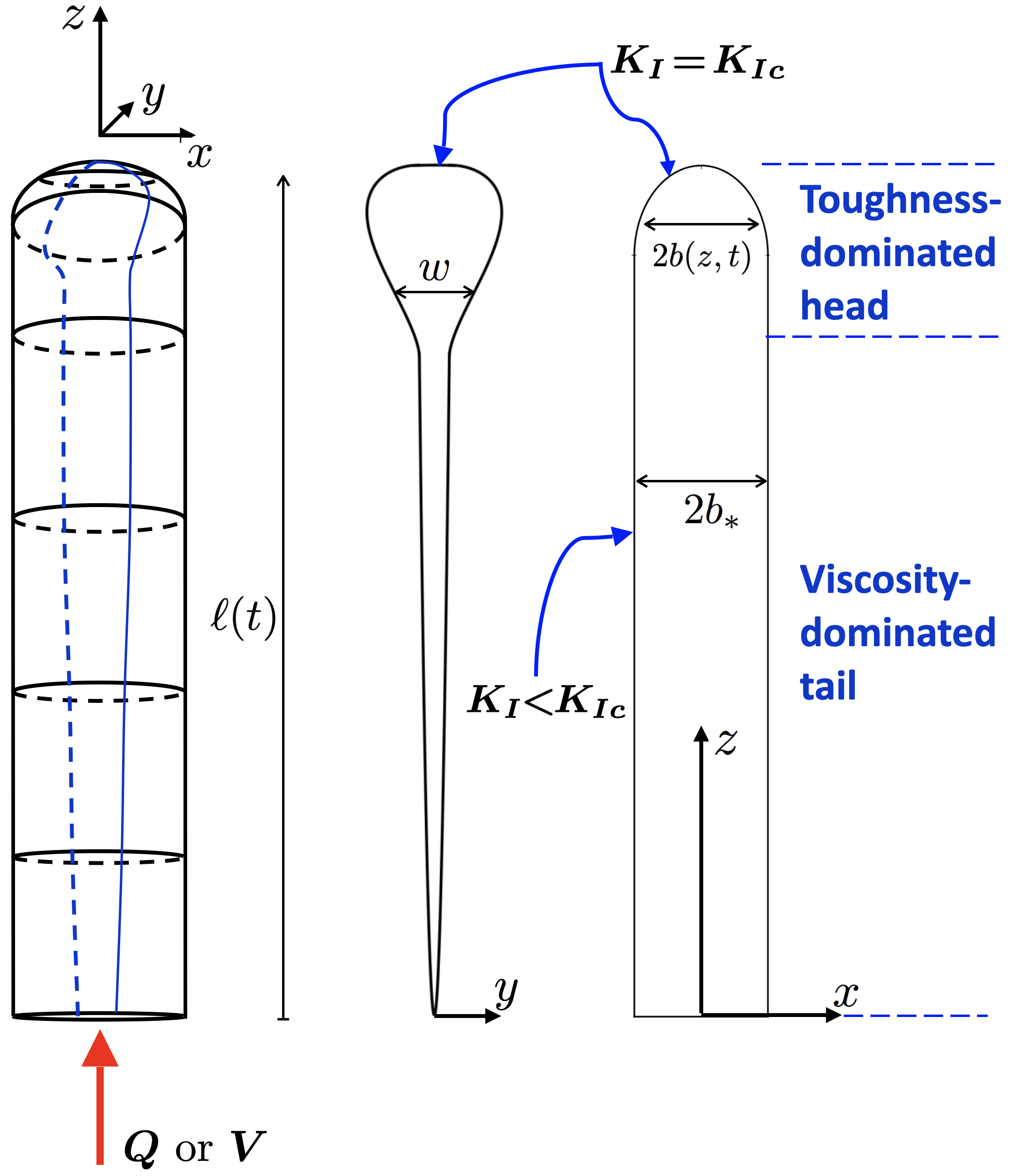
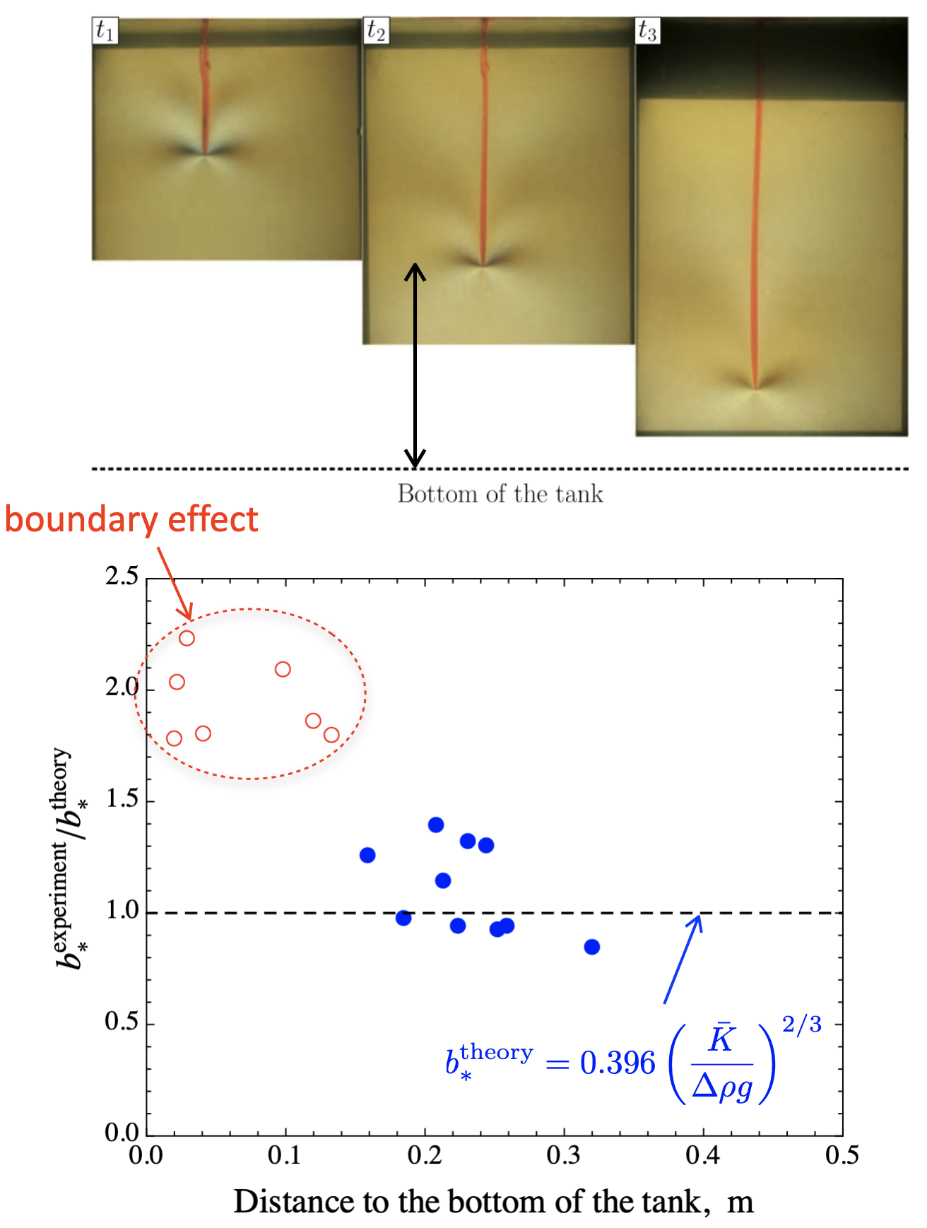
In this paper we present a mechanical model of a 3D buoyant hydraulic fracture with spontaneously developing breadth, as was first reported by Garagash and Germanovich (2014); Germanovich et al. (2014). The model takes a cue from observation of experimental dikes (Takada, 1990; Heimpel and Olson, 1994; Taisne and Tait, 2009) that the fracture breadth is generated by the fracturing process in the head of the dike, and remain nearly stationary in the tail region behind the head (Fig 1).
(a) (b)
(b)
(c)
We start in Section 2 of the paper with formulating a full 3D model for a buoyant fluid-driven crack, followed in Section 3 with the reduction of this model for the case of a small breadth-to-length ratio, similar to the so-call PKN model for non-buoyant lateral propagation of finger-like (or blade) fluid-driven cracks. Here we provide a general evolution of this PKN-like model for a finger-dike, as well as, develop the asymptotic, ’large-toughness’ head-tail structure, with the explicit asymptotic solutions for the toughness-dominated, hydrostatic head and viscosity-dominated tail. Stationary breadth of the finger-like dike cannot be determined within the PKN-like model, and have to be prescribed there. Section 4 therefore develops the explicit 3D solution for the hydrostatic dike head (Weertman’s pulse in 3D), including that for the dike breadth, which can be used to inform the PKN-like model of Section 3. Comparison of the dike-head solution to the experiments are also discussed. Section 5 follows with examples of the finger-dike propagation solutions in the PKN-like approximation with breadth informed by the dike-head solution of Section 4. Main results of the paper are summarized in Section 6.
2 Formulation
We consider a crack propagating in the fluid “buoyancy direction”, ( the gravity vector), aligned here with the -axis, from a source at the origin of the coordinate frame (Fig 2). The crack plane is perpendicular to the direction of the minimum in-situ stress (-axis), which is assumed to vary along along the lithostatic gradient, , where ’’ corresponds to the sense of buoyancy, , and is the reference stress level corresponding to the value at . (Stress is positive in compression). The fracture surface is specified by with , where is the local breadth of the crack and is its length.
It proves convenient to make use of the following effective material parameters
| (1) |
related by a numerical factor to the solid toughness , the solid plane-strain elastic modulus , and the dynamic fluid viscosity .
The crack opening (= displacement discontinuity in the -direction) is related to the net fluid pressure in the crack, , by a non-local relation of elasticity (e.g. Hills et al., 1996)
| (2) |
where is an elastic modulus, (1), and time was suppressed from the list of arguments for brevity. The integral in (2) is hypersingular and is understood in the Hadamard sense.
The flow of incompressible Newtonian fluid in the crack is governed by the local continuity,
| (3) |
and by the Poiseuille law for the flow velocity ,
| (4) |
where . We further assume slowly varying (if at all) breadth of a buoyancy-driven fracture, and, thus, negligible lateral components of fluid velocity and pressure gradient,
| (5) |
This assumption may possibly breakdown at early stages of the fracture when its breadth and length are comparable.
We further assume that the fluid wets the entire crack (i.e. the lag between the fluid and the fracture edge is negligible (e.g. Rubin, 1993; Garagash and Detournay, 2000) and the fluid velocity there is identical to the edge velocity)
| (6) |
Under this assumption and assuming that the leak-off into the rock is negligible, the fluid source condition can be equivalently formulated as the statement of global fluid continuity,
| (7) |
where is the cumulative volume of the injected fluid.
Adopting linear elastic fracture mechanics, the fracture propagation in mobile equilibrium requires that the local opening-mode stress intensity factor along the fracture edge is equal to or less than the solid toughness along the propagating and stationary parts of the front, respectively,
| (8) |
This propagation condition can also be conveniently rephrased in terms of the asymptotic behavior of the crack opening near (the propagating part of) the crack edge as (Irvin, 1957)
| (9) |
where is a toughness parameter, (1), and in the crack opening in a cross-section normal to the front ( is the distance from the front within the cross-section). Along the non-propagating part of the crack edge, .
3 Propagation of Finger Crack with Stationary Breadth (PKN-Approximation)
3.1 Preliminaries
It has been observed in laboratory experiments in gelatin (Takada, 1990; Heimpel and Olson, 1994; Taisne and Tait, 2009) that the fracture breadth is nearly stationary when the fracturing process near the fracture head (), that “generates” the final breadth of the crack , is dominated by the solid toughness, as opposed to the dissipation in the viscous fluid flow in the crack. This is symptomatic of buoyancy-driven cracks which tend to have maximum opening in the head region, which, in turn, minimizes the viscous losses there.
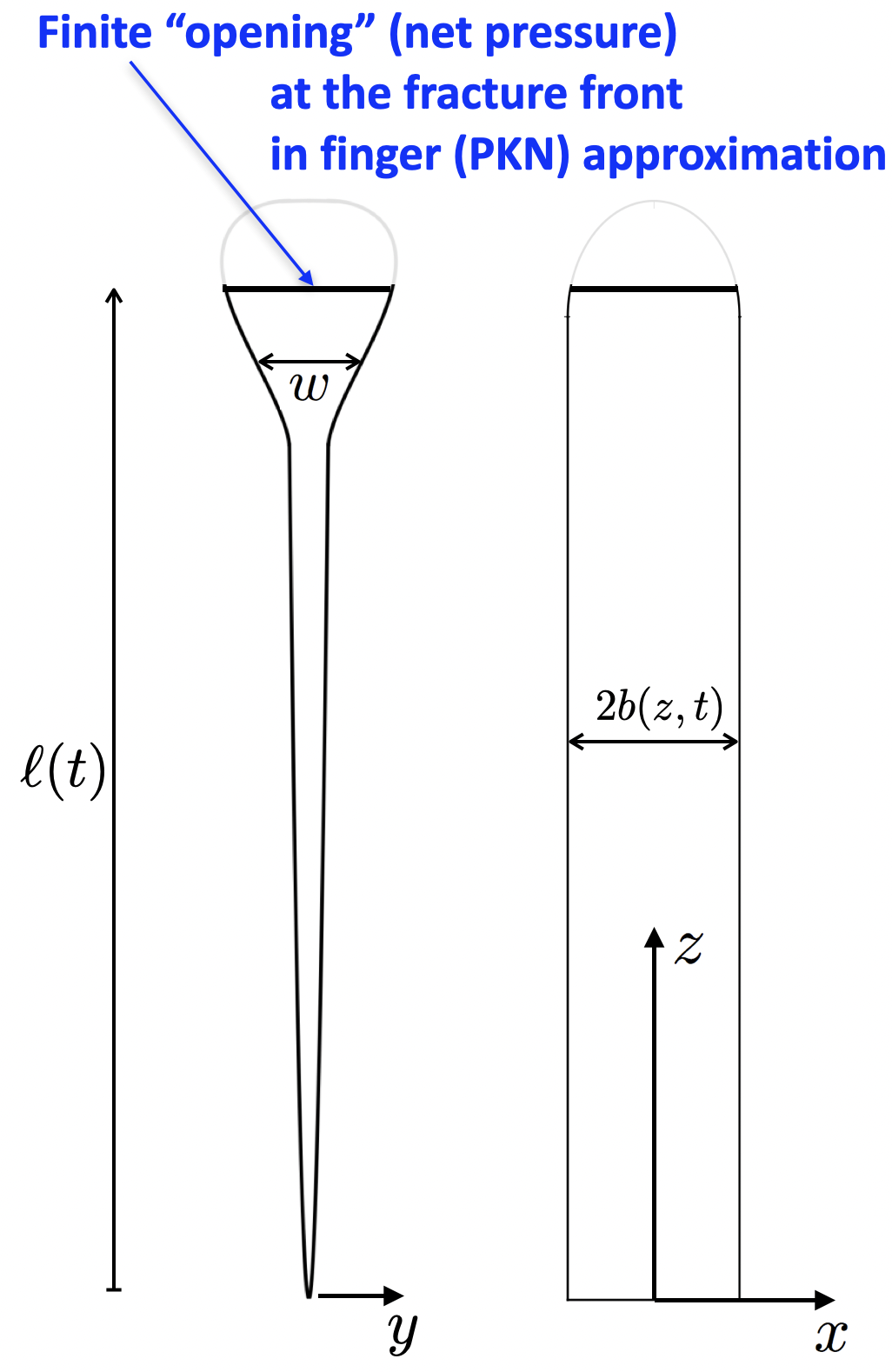
We turn to study such buoyancy-driven cracks with a small aspect (breadth-to-length) ratio,
| (10) |
The determination of the actual value of the stationary breadth will require explicit consideration of the structure of the “head region”, which is delayed until the next section. We only note at this point that the breadth is expected to be invariant with depth (fracture height) if the rock properties are depth-independent. Conversely, if the fracture toughness and/or the rock modulus and/or rock density (and thus density mismatch between the fluid and the rock) are depth dependent (which is conceivable if kilometers high dikes/fracture are considered), then the breadth is expected to vary with depth. Thus, in what follows, we allow for the rock modulus and the rock toughness are to be some predetermined functions of depth.
For a finger-like crack, , and “slowly” varying opening along the crack length, , the convolution kernel in (2) can be approximated as
which then allows to reduce (2) to its plane-strain equivalent (e.g. Bilby and Eshelby, 1968)
| (11) |
Once again, this approximation breaks down in the vicinity of the crack “tips” (i.e., near and ).
Since the pressure is approximately equilibrated along the breadth, (5), , eq. (11) yields classical elliptical crack opening that can be expressed as
| (12) |
where is the breadth-averaged opening
| (13) |
and time was omitted from the list of arguments in , , and .
Integrating the fluid flow equations along the crack breadth (and using the zero lag condition (6)) yields
| (14) |
where is the cross-section averaged flow rate
| (15) |
where is a dynamic viscosity parameter, as defined earlier in (1).
The zero fluid lag condition applied at the “tip” yields
| (16) |
while the global fluid volume balance reduces to:
| (17) |
The closure of the approximate model (12-17), which is in so far equivalent to the classical PKN model of a hydraulic fracture with restricted breadth (Perkins and Kern, 1961; Nordgren, 1972; Kemp, 1990), requires specifying an additional constraint or boundary condition. Naturally, the latter has to do with the crack propagation condition. Unfortunately, since the solution in the head of the fracture is not resolved by the current approximation, the propagation condition in the form (8) can not be applied directly. Instead, the “net” propagation criterion for the fracture head can be established from estimating the global energy release rate in extending the finger crack and equating it to the fracture energy (Sarvaramini and Garagash, 2015; Garagash, 2022). This “net” propagation constraint is:
| (18) |
We emphasize again that the approximate model of a finger crack includes the crack breadth . Therefore, when is known a priori, such as in the case of a hydraulic fracture propagation in a layer sandwiched between tougher/stiffer layers and/or layers subjected to higher compressive stress, this model is complete (Sarvaramini and Garagash, 2015; Garagash, 2022). Otherwise, as is true for a buoyant crack in a homogeneous rock, is not known a priori, and is a part of the solution in the fracture head (Section 4).
3.2 Scaling (depth-independent rock properties and fracture breadth)
Let us nondimensionalize the field variables with respect to the scales
| (19) |
which are predicated on a single lengthscale , chosen here as the buoyancy length (Lister and Kerr, 1991)
| (20) |
Expanded form of the scales (19) with (20) is:
| (21) |
Elasticity, fluid continuity and the Poiseuille’s equations can be rewritten in units of (19), or, conversely, in the normalized form as
| (22) |
Plugging the first and the third into the second in (22) we have
| (23) |
This non-linear PDE is subjected to the following global and boundary conditions:
| (24) |
| (25) |
The normalized solution and of (23-25) depends on the normalized injected fluid volume , and normalized fracture breadth .
The formulation for the case when the rock properties and the fracture breadth vary with depth is given in Appendix A.
3.3 Normalized Solution using Scales (19)
Numerical method of lines is used to solve the non-linear PDE (23) with boundary conditions (24) and (25), as detailed in Appendix B. The numerical solution reveals at large enough times an asymptotic structure comprised of a hydrostatic head region, where viscous stresses are negligible compared to the elastic ones and solution is stationary in the frame moving with the crack tip, and a viscous tail region, where the elastic stress is negligible. These two asymptotic head and tail solutions are discussed below.
3.3.1 Outer Solution for the Buoyant (Hydrostatic) Head
Hydrostatic net pressure
| (26) |
Applying the propagation condition at the tip () ,
| (27) |
The volume of the head is
| (28) |
In dimensional terms, i.e. restoring “units” (19) in the above two expressions, we have
3.3.2 Asymptotic Solution for the Viscous Tail
This is the case analyzed for a plane-strain (infinite breadth) dyke by Spence et al. (1987) and Lister (1990) in the case of constant fluid injection rate and by Spence and Turcotte (1990) in the case of constant injected fluid volume. The solution for a finite breadth crack considered here is different from these plane-strain solutions by numerical prefactors only. In the viscous tail, , the net pressure gradient is negligible compared to the buoyancy gradient over most of the fracture length, i.e. , and a similarity solution can be obtained by usual methods in the form , for an arbitrary injection power-law with . The solutions for the two cases of most interest are given below.
Constant injection rate :
| (29) |
Constant volume release :
| (30) |
where is the constant volume of the tail, and is the maximum net pressure in the tail, at the juncture with the head (we refer to as the “neck”).
Couple comments about these solutions are in order. Since the volume of the fracture head () is stationary, the volume of the tail () expands at the rate of fluid injection. The two solutions satisfy the tail continuity equation and the velocity condition at the juncture between the expanding tail and the stationary head, at .
Furthermore, in order for the asymptotic dike structure to be realizes (i.e., hydrostatic head “attached to” the viscous tail with stationary breadth), the pressure in the viscous tail should not exceed the fracturing value at the tip, (or in dimensional terms, ). More precisely, to avoid expansion of the tail breadth, pressure there should not exceed the “breadth fracturing” value for a uniformly pressurized plane-strain cross-section through (along?) the breadth, (or in dimensional terms, ). This requires, that, in the injection case, the normalized injection rate does not exceed a critical value
| (31) |
and in the shut-in case, the normalized time exceeds the critical one (when the pressure at falls below the breadth fracturing value)
| (32) |
The dimensional form of these constraints obtained by multiplying the right hand sides by the injection rate scale .
In dimensional terms, the net-pressure is related to the average opening by (13) and the above normalized asymptotic solutions translate to the dimensional expressions for the tail length and width using corresponding scales (19). In the interest of comparing these solutions to their two-dimensional (infinite breadth dike) counterparts, we express the former in terms of the equivalent 2-D rate and 2-D volume (area), respectively,
as
These 3D dikes expressions are equivalent to the corresponding expressions for plane-strain dikes (e.g., equations (2.4) and (6.7) of Roper and Lister, 2007, respectively) upon replacing the viscosity parameter by . This, for example, translates to a factor difference between the values of the length of the viscous tail of a finite- and an infinite- breadth dikes.
3.4 Asymptotic solution with partial head
The asymptotic solution with the full hydrostatic head attached to the viscous tail is realized when the neck pressure (opening), i.e., as previously defined maximum pressure in the tail occurring at the juncture of the tail and the head, is negligible compared to the prevailing pressure in the head, i.e. . This asymptotic framework can be approximately extended to the case when is not vanishingly small by “attaching” the partial head (“circumcised” at the value of pressure equal to ) to the viscous tail, such that the partial head size and volume are
where is stationary for a constant injection rate, (29), and decreasing with time for a constant volume release, (30). In the latter case, since evolves with time, so does , which now satisfies an implicit equation
Corresponding solution with non-stationary volume in the tail is no longer strictly self-similar, yet, we hypothesize that the constant solution formally used with a slowly varying may still yield an adequate approximation…
4 The Full Solution for the Buoyant (Hydrostatic) Head
4.1 Full Numerical Solution
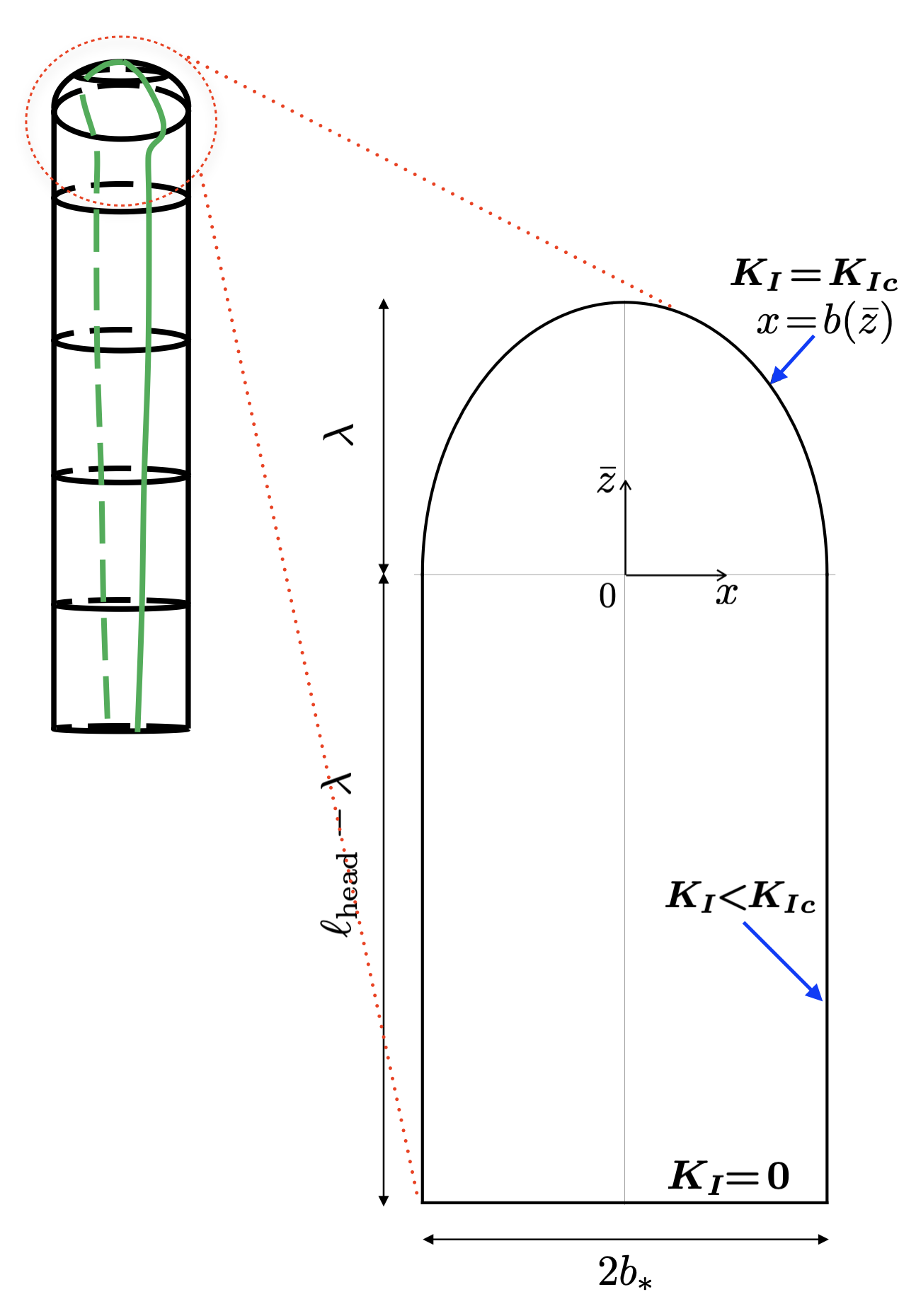
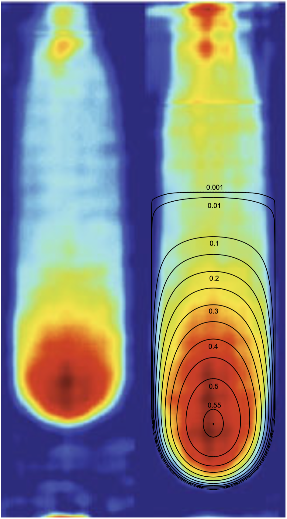
Here we look for the full solution in the fracture head (which approximate solution we studied in the previous section), including the yet unknown value of the stationary breadth away from the tip and the unknown “build-up” in the near-tip region of a priori unknown vertical extent , where the fracture breadth gradually expands towards the terminal value to accommodate the vertical propagation (Figure 4). We further make use of local coordinate with the origin situated at the boundary between the laterally expanding (, ) and laterally stationary (, ) parts of the fracture edge.
| (33) |
while the net pressure is hydrostatic in the head
| (34) |
where is yet unknown constant. The normalized conditions along the expanding, (9), and the stationary parts of the fracture edge are, respectively,
| (35) |
| (36) |
where is, as previously, the opening distribution in the cross-section normal to the fracture edge. Finally, these are complemented by the condition of smooth fracture edge, specifically at the juncture ,
| (37) |
We use the piecewise-constant displacement discontinuity method, as further detailed in Appendix C, to numerically solve elasticity integral equation (33) together with constraints (35-37) for the terminal fracture breadth and the reference pressure value, respectively,
| (38) |
the crack opening show on Figure 5, and the fracture breadth distribution
in the laterally-expanding part (of the head region) of extent
The fracture breadth is stationary, , in the remainder of the head region of extent
The true extent of the head region is therefore
| (39) |
We note that the net pressure at the tail-end of the head, i.e. at , has a negative value , which owes to the non-local 3D crack effects there. (Departure from the PKN assumption, which would have required zero net-pressure there).
The volume of the head is
| (40) |
4.2 PKN-Approximation of the Head
The PKN-approximation of the solution in the head, as shown on on Figure 5b by dashed line, corresponds to , where in the head is taken from the full head solution (34) with (38). The PKN approximation of the advancing front location follows from the propagation condition , while the back (reseeding) front corresponds to the closure condition . Although the validity of the PKN assumption is at best questionable in the head region, which extent is only about 2.5 times larger than its terminal breadth , (39), the PKN solution for the breadth-averaged opening starts to track the full numerical solution some distance behind the tip (Figure 5b). What is however even more remarkable is that the equivalent PKN volume of the head region (see (28) and (38)), is in very good agreement (% different) with the full numerical solution (40). This lands support to the PKN solution for the finger crack (including the hydrostatic head, viscous tail, and the transition between the two) developed in Section 3, as long as the head region is at least partially developed, see constraints (31) for the constant injection rate and (32) for the constant volume release cases.
4.3 Comparison to the Weertman’s 2D Head Solution
Draw comparisons to Weertman’s 2D pulse solution (Weertman, 1971)….
where
is the half-length of the pulse ( correspond to advancing/reseeding tips in the coordinate system used in the Weertman’s solution). In our notation, where is a buoyancy length, and .
In order compare the 2D and 3D pulse solution, we need to relate the corresponding coordinate frames, i.e., and , respectively. We choose to do so by requiring that the net pressure distributions in the two solutions are identical, i.e., , which leads to .
The normalized volume of the Weertman’s 2-D pulse is equal to , which approximates well the equivalent 2-D-volume of the 3-D pulse, . This result, taken together with the approximate correspondence of the 2-D and 3-D viscous tail solutions obtained earlier, suggests that the 2-D framework provides a good approximation (within 10% in terms of the dike length, width, and head vs. tail volume partition) of the 3-D dike solution as long as the appropriate (obtained from the 3-D hydrostatic head solution) value of the stationary breadth is used to convert the dike’s volume to its 2-D proxy.
4.4 Comparison with Laboratory Experiments
5 Application to Dikes with Fixed Volume
We consider an example of dike driven by a fixed volume of fluid released at the source over some time . Dike dynamics is described by the asymptotic head-tail solution discussed in the above for , if the release volume is larger than the volume accommodated in the dikes head, i.e. and thus
where head’s volume is fully defined by the solids property and buoyancy gradient
Otherwise, i.e. when , dikes is expected to arrest in the neighborhood of the source.
Dike dynamics is governed by the viscosity-dominated, slowing growth of the dike’s tail
This predicts slowing, but not arresting dynamics, with the ascent rate scaling with the tail’s volume given by the excess of the injected volume over the volume of the head. In reality, eventual dike arrest can be precipitated by changes of the buoyancy condition in the shallower crust, and by the effective loss of dike’s fluid volume to freezing in the thinning tail.
6 Conclusions
A particular solution for a 3D (finite breadth) gravity driven hydraulic fracture is developed. Solution has a similar structure to that of 2D (infinite breadth) dikes, consisting of:
-
•
an extensive “tail”, stretching and thinning in time, with a stationary breadth, which solution is dominated by the viscous fluid flow and characterized by negligible elastic interactions
-
•
a compact hydrostatic “head” dominated by the rock toughness and elastic interactions, a 3D analog of “Weertman pulse”, which determines the terminal fracture breadth
Dyke propagation dynamics is governed by by the viscous fluid flow in a thin tail, i.e. “tail wags the dog…” (Stevenson, 1982). Yet, for 3D dykes, “dog’s head” plays a crucial role in the dynamics, as it creates the fracture breadth, and thus directly impacts the tail solution and dyke dynamics by partitioning the injected fluid volume between the head and the tail and by constraining the geometry of the tail, the dynamics of the fluid flow therein, and thus the propagation of the dike.
Contrary to some previous suggestions, fixed-volume-release dykes have slowing dynamics, but do not arrest, unless encounter tougher or softer enough ground resulting in the head-volume expansion accommodating entire fracture fluid volume, i.e. completely depleting dyke’s tail.
References
- Abramowitz and Stegun [1964] M. Abramowitz and I. A. Stegun, editors. Handbook of Mathematical Functions with Formulas, Graphs, and Mathematical Tables. Applied Mathematics Series, 55. U. S. Govt. Print. Off., Washington, D.C., 1964.
- Bilby and Eshelby [1968] B.A. Bilby and J.D. Eshelby. Dislocations and the theory of fracture. In H. Liebowitz, editor, Fracture, an Advanced Treatise, volume I, chapter 2, pages 99–182. Academic Press, New York NY, 1968.
- Garagash [2022] D. I. Garagash. Fluid-driven crack tunneling in a layer. J. Appl. Mech., submitted, 2022.
- Garagash and Detournay [2000] D. I. Garagash and E. Detournay. The tip region of a fluid-driven fracture in an elastic medium. ASME J. Appl. Mech., 67(1):183–192, 2000.
- Garagash and Germanovich [2014] Dmitry Garagash and Leonid Germanovich. Gravity driven hydraulic fracture with finite breadth. In A. Bajaj, P. Zavattieri, M. Koslowski, and T. Siegmund, editors, Proceedings of the Society of Engineering Science 51st Annual Technical Meeting, October 1-3, 2014, West Lafayette, 2014. Purdue University Libraries Scholarly Publishing Services.
- Germanovich et al. [2014] L. N. Germanovich, D. I. Garagash, L. C. Murdoch, and M. Robinowitz. Gravity-driven hydraulic fractures. volume 95, pages H53C–0874, 2014.
- Heimpel and Olson [1994] M. Heimpel and P. Olson. Buoyancy-driven fracture and magma transport through the lithosphere: Models and experiments. In M. P. Ryan, editor, Magmatic Systems, volume 57 of Int. Geophys. Ser., chapter 10, pages 223–240. Academic, San Diego, Calif., 1994.
- Hills et al. [1996] D.A. Hills, P.A. Kelly, D.N. Dai, and A.M. Korsunsky. Solution of Crack Problems. The Distributed Dislocation Technique, volume 44 of Solid Mechanics and its Applications. Kluwer Academic Publ., Dordrecht, 1996.
- Irvin [1957] G. R. Irvin. Analysis of stresses and strains near the end of a crack traversing a plate. ASME J. Appl. Mech., 24:361–364, 1957.
- Kemp [1990] L. F. Kemp. Study of Nordgren’s equation of hydraulic fracturing. SPE Prod. Eng., pages 311–314, August 1990.
- Lister [1990] J. R. Lister. Buoyancy-driven fluid fracture: The effects of material toughness and of low-viscosity precursors. J. Fluid Mech., 210:263–280, 1990.
- Lister and Kerr [1991] J. R. Lister and R. C. Kerr. Fluid-mechanical models of crack propagation and their applications to magma transport in dykes. J. Geophys. Res., 96(B6):10,049–10,077, 1991.
- Nordgren [1972] R. P. Nordgren. Propagation of vertical hydraulic fractures. J. Pet. Tech., 253:306–314, 1972. (SPE 3009).
- Peirce and Detournay [2008] A. Peirce and E. Detournay. An implicit level set method for modeling hydraulically driven fractures. Computer Meth. Appl. Mech. Eng., 197:2858–2885, 2008.
- Perkins and Kern [1961] T. K. Perkins and L. R. Kern. Widths of hydraulic fractures. J. Pet. Tech., Trans. AIME, 222:937–949, 1961.
- Rivalta et al. [2015] E. Rivalta, B. Taisne, A.P. Bunger, and R.F. Katz. A review of mechanical models of dike propagation: Schools of thought, results and future directions. Tectonophysics, 638:1 – 42, 2015. ISSN 0040-1951. doi: https://doi.org/10.1016/j.tecto.2014.10.003. URL http://www.sciencedirect.com/science/article/pii/S0040195114005174.
- Roper and Lister [2007] S. M. Roper and J. R. Lister. Buoyancy-driven crack propagation: the limit of large fracture toughness. J. Fluid Mech., 580:359–380, 2007. doi: 10.1017/S0022112007005472.
- Rubin [1993] A. M. Rubin. Tensile fracture of rock at high confining pressure: Implications for dike propagation. J. Geophys. Res., 98(B9):15,919–15,935, 1993.
- Rubin [1995] A. M. Rubin. Propagation of magma-filled cracks. Annu. Rev. Earth Planet Sci., 23:287–336, 1995.
- Sarvaramini and Garagash [2015] E. Sarvaramini and D. I. Garagash. Breakdown of a pressurized finger-like crack in a permeable rock. J. Appl. Mech., 82(6):061006, 2015.
- Spence and Turcotte [1990] D.A. Spence and D.L. Turcotte. Buoyancy-driven magma fracture: a mechanism for ascent through the lithosphere and the emplacement of diamonds. J. Geophys. Res., 95(B4):5133–5139, 1990.
- Spence et al. [1987] D.A. Spence, P.W. Sharp, and D.L. Turcotte. Buoyancy-driven crack propagation: a mechanism for magma migration. J. Fluid Mech., 174:135–153, 1987.
- Stevenson [1982] D. J. Stevenson. Migration of fluid-filled cracks: applications to terrestrial and icy bodies. Lunar Planet. Sci., XIII:768–769, 1982.
- Tada et al. [2000] H. Tada, P. C. Paris, and G.R. Irwin. The Stress Analysis of Cracks Handbook. ASME Press, 3rd edition, 2000.
- Taisne and Tait [2009] B. Taisne and S. Tait. Eruption versus intrusion? Arrest of propagation of constant volume, buoyant, liquid-filled cracks in an elastic, brittle host. J. Geophys. Res., 114:B06202, 2009. doi: 10.1029/2009JB006297.
- Taisne et al. [2011] Benoît Taisne, Stephen Tait, and Claude Jaupart. Conditions for the arrest of a vertical propagating dyke. Bulletin of Volcanology, 73(2):191–204, 2011.
- Takada [1990] A. Takada. Experimental study on propagation of liquid-filled crack in gelatin: shape and velocity in hydrostatic stress condition. J. Geophys. Res., 95(B6):8471–8481, 1990.
- Weertman [1971] J. Weertman. Theory of water-filled crevasses in glaciers applied to vertical magma transport beneath oceanic ridges. J. Geophys. Res., 76(5):1171–1183, 1971.
Appendix A PKN-like Gravity Fracture for Depth-Dependent Rock Properties
Let us nondimensionalize the field variable with respect to the scales
| (41) |
where
| (42) |
is the buoyancy lengthscale [Lister and Kerr, 1991] expressed in terms of reference values , , and of the density mismatch , the rock toughness , and the rock modulus , respectively. (Functions , , and define the depth-dependence of the rock properties).
The normalized elasticity equation (13), the fluid continuity and the Poiseuille law can be written in units of (41), respectively, as
| (43) |
Plugging the first and the third into the second
| (44) |
This non-linear PDE is subjected to the following global and boundary conditions:
| (45) |
| (46) |
The normalized solution and of (44-46) depends on the normalized injected fluid volume , normalized buoyancy , elasticity , and toughness parameters, and the normalized fracture breadth .
Appendix B Numerical Method of Lines for Solution of PKN-like Fracture
Non-linear PDE (23) is to be solved with the b.c. (24) and (25) for the evolution of the pressure over the crack with a priori unknown length . To avoid dealing explicitly with an unknown spatial domain, we normalize the domain to the interval by passing to the normalized coordinate
The governing equations translate to
| (47) |
where the partial time derivative is now understood to be taken at a fixed and is the crack tip velocity. Fluid flow boundary conditions read
| (48) |
where only two of the three conditions are independent. The fracture propagation condition reads
| (49) |
Round-up of the numerical scheme:
-
•
Discretize the interval in equally-spaced points (including the end points, and ). In view of the propagation condition (49), which prescribes the pressure at the last node, , we looking to determine the evolution in time of the unknowns (pressure at grid points , , and the fracture length ).
-
•
Evaluate lubrication equation (47) at the internal grid points using the second-order space finite differences. This leads to the ODEs for the pressure evolution at the internal grid points, i.e. , .
-
•
Evaluate two of the three relations (48): (i) global fluid volume balance, (ii) flow rate at the inlet, and (iii) flow velocity at the tip (equal to the crack tip velocity). Default choices are the rate of (i) expressed as an ODE for the pressure at the inlet, , and (iii), which provides an ODE for the crack length. Different choices are used for large-time shut-in problems, namely, the rate of (ii) with , is used to evaluate the pressure rate at the inlet, and the rate of (i) is now used to evaluate the fracture velocity. The latter change is necessitated by the deterioration of the accuracy of the finite difference employed in (iii) to evaluate the fluid velocity at the crack tip, as fracture slows down and conditions in the tip region approach that in the hydrostatic head asymptote.
The resulting system of ODEs is solved starting from an artificial initial state , , and at small, but non-zero , that is consistent with the propagation condition and the global fluid balance. The impact of the choice of is negligible on the solution for .
As discussed in the main text, the finger-like buoyant fracture develops an asymptotic structure at large time consisting of the stationary hydrostatic head, expanding viscous tail, and, in the case of the shut-in (i.e. fixed fluid volume release), another hydrostatic region at the crack inlet. The former and latter boundary regions are characterized by stationary () and decreasing () sizes, respectively, and, thus, eventually become small compared to growing body (“viscous tail”) of the fracture. This necessitates using a rather large number of spatial nodes in order to resolve these two boundary layers and the overall fracture solution at large time.
Appendix C Displacement Discontinuity Methodology for Hydrostatic Fracture Head Solution
We use the piecewise-constant displacement discontinuity method to solve elasticity equation (33) at the collocation points located at the centers of the uniformly sized rectangular grid elements [e.g. Peirce and Detournay, 2008]. Let us use a pair of indices ’’ to refer to the rectangular boundary element with the center at and dimensions , and characterized by constant opening . Then elasticity equation (33) can be evaluated at the center of a -elelment in the form
| (50) |
where the influence matrix is defined by
and the summation convention over repeating indices is used. Since pressure is distributed hydrostatically, (34), we have for the -element
| (51) |
We approximate the unknown fracture front in the tip region () by an oval shape
| (52) |
where the maximum breadth , the length of the near-tip region , and parameter are parts of the solution. The form (52) automatically satisfies the constraints at the two ends of the tip region: , , and .
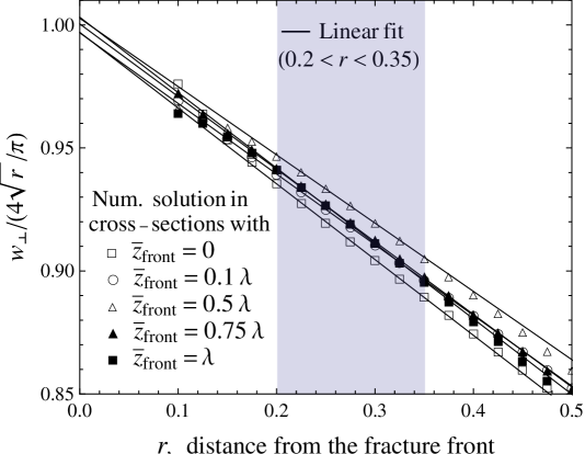
To implement the propagation condition (35), an accurate evaluation of the opening near the edge (the stress intensity factor) is required. The numerical resolution of the constant DD method immediately near the crack edge (the first few elements) is inadequate, i.e. opening some distance away from the edge is to be used to determine the tip asymptotics and the stress-intensity factor there. In practice, we sample the numerical solution in the cross-section normal to a point of interest on the fracture edge at distances from the edge, and fit the sampled opening values by a linear combination of the first two asymptotic terms, . The coefficient is equivalent to the normalized stress intensity factor , and is required to be equal to the unity along the expanding part of the fracture edge, (35). Thus, in the numerical solution of (50-51), we search for values of parameters and of the “oval-shape” (52), the value of the terminal fracture breadth , and the reference pressure value which minimize along the expanding part of the fracture edge, (52). When carrying out the numerical solution, we actually rescale the space with regard to the unknown terminal breadth in order to fix the spatial domain of the solution. The unknown value of then assumes the meaning of the reciprocal of the unknown hydrostatic pressure gradient in the appropriately rescaled (51).
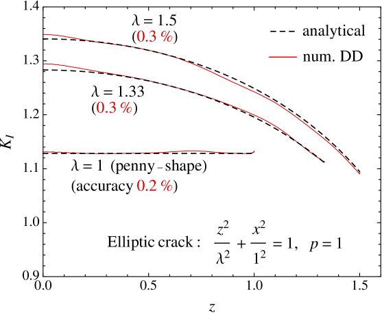
The final note on the numerical implementation is related to the allocation of the rectangular grid elements to the crack foot-print near its curved edge, with . The choice of these “edge” elements happen to have a considerable impact on the computed values of the stress intensity factor. We set the grid element allocation criteria by requiring the intersection area between the grid element and the crack footprint exceeds a particular fraction of the element’s area (). To determine the optimum area fraction we test the numerical (DD) solution for the stress-intensity factor (determined by using the method outlined in the above) against the analytical solution for a uniformly pressurized () crack with an elliptical footprint [e.g. Tada et al., 2000]
where and are the semi-axises of the elliptical crack and is the complete elliptic integral of the second kind [Abramowitz and Stegun, 1964].
We find the optimum threshold value for the grid element’s area fraction to be 0.77 (77% of a grid element’s area belongs to the crack footprint). Figure 8 shows that the numerical (DD) and analytical solutions for various values of the crack footprint aspect ratio differ by not more than .