Note on Minimization of Quasi \Mnat-convex Functions111 This work was supported by JSPS KAKENHI Grant Numbers JP23K11001 and JP23K10995.
Abstract
For a class of discrete quasi convex functions called semi-strictly quasi \Mnat-convex functions, we investigate fundamental issues relating to minimization, such as optimality condition by local optimality, minimizer cut property, geodesic property, and proximity property. Emphasis is put on comparisons with (usual) \Mnat-convex functions. The same optimality condition and a weaker form of the minimizer cut property hold for semi-strictly quasi \Mnat-convex functions, while geodesic property and proximity property fail.
1 Introduction
In this paper, we deal with a class of discrete quasi convex functions called semi-strictly quasi \Mnat-convex functions [2] (see also [10]). The concept of semi-strictly quasi \Mnat-convex function is introduced as a “quasi convex” version of \Mnat-convex function [9], which is a major concept in the theory of discrete convex analysis introduced as a variant of M-convex function [5, 6, 8]. Application of (semi-strictly) quasi \Mnat-convex functions can be found in mathematical economics [2, 11] and operations research [1].
An M-convex function is defined as a function satisfying a certain exchange axiom (see Section 4.2), which implies that the effective domain is contained in a hyperplane of the form for some . Due to this fact, it is natural to consider the projection of an M-convex function to the -dimensional space along a coordinate axis, which is called an \Mnat-convex function. A nontrivial argument shows that an \Mnat-convex function is characterized by the following exchange axiom:
(\Mnat-EXC) , , such that
(1.1)
where , is the characteristic vector of , , and
The inequality (1.1) implies that at least one of the following three conditions holds:
| (1.2) | |||
| (1.3) | |||
| (1.4) |
Using this, a semi-strictly quasi \Mnat-convex function (s.s. quasi \Mnat-convex function, for short) is defined as follows: is called an s.s. quasi \Mnat-convex function if it satisfies the following exchange axiom:
(SSQM♮) , , satisfying at least one of the conditions (1.2), (1.3), and (1.4).
The main aim of this paper is to investigate fundamental issues relating to minimization of an s.s. quasi \Mnat-convex function. It is known that minimizers of an M-convex function have various nice properties (to be described in Section A.1 of Appendix) such as
optimality condition by local optimality,
minimizer cut property,
geodesic property,
proximity property.
The definition of \Mnat-convex function implies that these properties of M-convex functions are inherited by \Mnat-convex functions, as shown in Section 2. In this paper, we examine which of the above properties are satisfied by s.s. quasi \Mnat-convex functions. For each of the properties, if it holds for s.s. quasi \Mnat-convex functions, we describe the precise statement of the property in question and give its proof; otherwise, we provide an example to show the failure of the property.
It is added that there is a notion called “s.s. quasi M-convex function” [8, 10], which corresponds directly to M-convexity. Although M-convex and \Mnat-convex functions are known to be essentially equivalent, it turns out that their quasi-convex versions, namely, s.s. quasi M-convexity and s.s. quasi \Mnat-convexity, are significantly different. We also discuss such subtle points in Section 4.2.
2 Properties on Minimization of Quasi \Mnat-convex Functions
2.1 Optimality Condition by Local Optimality
In this section we consider an optimality condition for minimization in terms of local optimality and also a minimization algorithm based on the optimality condition. Before dealing with quasi \Mnat-convex functions, we describe the existing results for \Mnat-convex functions.
A minimizer of an \Mnat-convex function can be characterized by the local minimality within the neighborhood consisting of vectors with .
Theorem 2.1 (cf. [5, Theorem 2.4], [7, Theorem 2.2]).
Let be an \Mnat-convex function. A vector is a minimizer of if and only if
| (2.1) |
Theorem 2.1 makes it possible to apply the following steepest descent algorithm to find a minimizer of an \Mnat-convex function.
Algorithm BasicSteepestDescent
Step 0: Let be an arbitrarily chosen initial vector. Set .
Step 1: If for every , then output and stop.
Step 2: Find that minimize .
Step 3: Set and go to Step 1.
Corollary 2.2 (cf. [12]).
For an \Mnat-convex function with , Algorithm BasicSteepestDescent finds a minimizer of in a finite number of iterations.
The optimality condition for \Mnat-convex functions in Theorem 2.1 can be generalized to s.s. quasi \Mnat-convex functions.
Theorem 2.3.
Let be a function satisfying (SSQM♮). A vector is a minimizer of if and only if the condition (2.1) holds.
The “only if” part of the theorem is easy to see. The “if” part is implied immediately by the following lemma.
Lemma 2.4.
Let be a function satisfying (SSQM♮). For , if , then there exist some and satisfying .
Proof.
Putting
we prove the lemma by induction on the pair of values . If and , then for some , and therefore the claim holds immediately.
Suppose and let . By (SSQM♮) applied to , , and , there exists some satisfying or (or both). In the former case, we are done. In the latter case, we can apply the induction hypothesis to and to obtain some and satisfying . The proof for the case is similar. ∎
It follows from Theorem 2.3 that we can also apply the steepest descent algorithm to find a minimizer of an s.s. quasi \Mnat-convex function.
Corollary 2.5.
For a function with satisfying (SSQM♮), Algorithm BasicSteepestDescent finds a minimizer of in a finite number of iterations.
2.2 Minimizer Cut Property
The minimizer cut property, originally shown for M-convex functions [12, Theorem 2.2] (see also Theorem A.2 in Appendix), states that a separating hyperplane between a given vector and some minimizer can be found by using the steepest descent direction at (i.e., vector with that minimizes ). By rewriting the minimizer cut property for M-convex functions based on the relationship between M-convexity and \Mnat-convexity, we obtain the following minimizer cut property for \Mnat-convex functions, where for .
Theorem 2.6 (cf. [12, Theorem 2.2]).
Let be an \Mnat-convex function with , and be a vector with . For a pair of distinct elements in minimizing the value , there exists some minimizer of satisfying
| (2.2) |
Other variants of the minimizer cut property of \Mnat-convex functions are given in Section 4.1, which capture the technical core of Theorem 2.6.
Using Theorem 2.6 we can provide an upper bound for the number of iterations in the following variant of the steepest descent algorithm, where is assumed to be bounded, and the integer interval always contains a minimizer of .
Algorithm ModifiedSteepestDescent
Step 0: Let be an arbitrarily chosen initial vector. Set .
Let be vectors such that .
Step 1: If for every with ,
then output and stop.
Step 2: Find with that minimize .
Step 3: Set , if , and if .
Go to Step 1.
We define the L∞-diameter of a bounded set by
Corollary 2.7 (cf. [12, Section 2]).
For an \Mnat-convex function with a bounded effective domain, Algorithm ModifiedSteepestDescent finds a minimizer of in iterations with .
While the number of iterations in the algorithm ModifiedSteepestDescent is proportional to the L∞-diameter of , the domain reduction approach in [12] (see Section 3.2; see also [8, Section 10.1.3]), combined with the minimizer cut property, makes it possible to speed up the computation of a minimizer.
Corollary 2.8 (cf. [12, Theorem 3.2]).
Let be an \Mnat-convex function with a bounded effective domain, and suppose that a function evaluation oracle for and a vector in are available. Then, a minimizer of can be obtained in time with .
Note that faster polynomial-time algorithms based on the scaling technique are also available for \Mnat-convex function minimization [13, 15].
An s.s. quasi \Mnat-convex function satisfies the following weaker statement than Theorem 2.6. To be specific, the inequality in the second case () of (2.2) is missing in (2.3) below, and the inequality in the third case () of (2.2) is missing in (2.3); an example illustrating this difference is given later in Example 2.12.
Theorem 2.9.
Let be a function with (SSQM♮) satisfying , and be a vector with . For a pair of distinct elements in minimizing the value , there exists some minimizer of satisfying
| (2.3) |
A proof of this theorem is given in Section 3.1.
Using Theorem 2.9 we can obtain the same upper bound for the number of iterations in the algorithm ModifiedSteepestDescent applied to s.s. quasi \Mnat-convex functions.
Corollary 2.10.
For a function with a bounded effective domain satisfying (SSQM♮), Algorithm ModifiedSteepestDescent finds a minimizer of in iterations with .
A combination of Theorem 2.9 with the domain reduction approach (described in Section 3.2) makes it possible to find a minimizer of an s.s. quasi \Mnat-convex function in time polynomial in and , provided that is an \Mnat-convex set. Note that the effective domain of an s.s. quasi \Mnat-convex function is not necessarily an \Mnat-convex set (see (3.11) in Section 3.2 for the definition of \Mnat-convex set).
Corollary 2.11.
Let be a function satisfying (SSQM♮), and suppose that the effective domain of is bounded and \Mnat-convex. Also, suppose that a function evaluation oracle for and a vector in are available. Then, a minimizer of can be obtained in time with .
A proof of this corollary is given in Section 3.2.
Example 2.12.
This example shows that the statement of Theorem 2.6, stronger than Theorem 2.9, is not true for s.s. quasi \Mnat-convex functions. Consider the function defined by
(see Figure 1). This function satisfies (SSQM♮) and has two minimizers and (denoted by in Figure 1).

2.3 Geodesic Property
Geodesic property of a function means that whenever a vector moves to a local minimizer in an appropriately defined neighborhood of , the distance to a nearest minimizer from the current solution decreases by , where is an appropriately chosen norm. It is known that M-convex functions have the geodesic property with respect to the L1-norm [14, Corollary 4.2], [3, Theorem 2.4]. We first point out that \Mnat-convex functions do not enjoy the geodesic property with respect to the L1-norm.
For a function and a vector , we define
| (2.4) | ||||
| (2.5) |
The following is an expected plausible statement of the geodesic property for \Mnat-convex functions with respect to the L1-norm.
Statement A: Let be a vector that is not a minimizer of . Also, let be a pair of distinct elements in minimizing the value , and define
(i)
There exists some that is contained in ;
we have , in particular.
(ii)
It holds that
However, neither (i) nor (ii) of Statement A is true for \Mnat-convex functions, as shown by the following example.
Example 2.13.
This example shows that Statement A is not true for \Mnat-convex functions. Consider a function given by
(see Figure 2), for which . Function satisfies the condition (\Mnat-EXC), and hence it is \Mnat-convex.

For , we have
We see that is a possible choice to minimize the value among all . Then, we have
That is, Statement A does not hold for this \Mnat-convex function . ∎
While Statement A fails for \Mnat-convex functions, an alternative geodesic property holds for \Mnat-convex functions, which can be obtained from the geodesic property for M-convex functions with respect to the L1-norm (see [14, Corollary 4.2], [3, Theorem 2.4]; see also Theorem A.3 in Appendix).
Let be a function with . For , we define
That is, is a kind of distance from to the nearest minimizer of , and is the set of the minimizers of nearest to with respect to this distance.
Theorem 2.14 (cf. [14, Corollary 4.2], [3, Theorem 2.4]).
Let be an \Mnat-convex function with , and be a vector that is not a minimizer of , i.e., . Also, let be a pair of distinct elements in minimizing the value , and define
| (2.6) |
(i)
There exists some that is contained
in ;
we have , in particular.
(ii)
It holds that
and
.
Note that the statement (i) immediately implies the minimizer cut property (Theorem 2.6) for \Mnat-convex functions. The statement (ii) implies that in each iteration of Algorithm BasicSteepestDescent applied to an \Mnat-convex function, the distance to the nearest minimizer reduces by two. This fact yields an exact number of iterations required by BasicSteepestDescent.
Corollary 2.15.
Let be an \Mnat-convex function with . Suppose that Algorithm BasicSteepestDescent is applied to with the initial vector . Then, the number of iterations is equal to .
In contrast, s.s. quasi \Mnat-convex functions do not enjoy the geodesic property in the form of Theorem 2.14, as illustrated in the following example.
Example 2.16.
This example shows that the statement of Theorem 2.14 is not true for s.s. quasi \Mnat-convex functions in the case of or . Consider the s.s. quasi \Mnat-convex function in Example 2.12 (see Figure 1), for which . For , we have
For , we have and
However, we have
Thus, the statements (i) and (ii) in Theorem 2.14 fail for . ∎
2.4 Proximity Property
Given a function , , and an integer , we consider the following scaled minimization problem:
It is expected that an appropriately chosen neighborhood of a global (or local) optimal solution of the scaled minimization problem (SP) contains some minimizer of ; such a property is referred to as a proximity property in this paper. It is known that M-convex functions enjoy a proximity property [4, Theorem 3.4] (see also Theorem A.4 in Appendix), which can be rewritten in terms of \Mnat-convex functions as follows:
Theorem 2.17 (cf. [4, Theorem 3.4]).
Let be an \Mnat-convex function and be an integer. For every vector satisfying
there exists some minimizer of satisfying
This theorem, in particular, implies that for every optimal solution of (SP), there exists some minimizer of such that .
In contrast, a proximity property of this form does not hold for s.s. quasi \Mnat-convex functions. Indeed, the following example shows that there exists a family of s.s. quasi \Mnat-convex functions such that the distance between an approximate global minimizer and a unique exact global minimizer can be arbitrarily large.
Example 2.18.
This example shows a function satisfying (SSQM♮) for which the statement of Theorem 2.17 does not hold. With an integer , define a function as follows (see Figure 3 for the case of ):
It can be verified that satisfies the condition (SSQM♮). Note that the value is constant for every with , while , and are strictly increasing with respect to in the interval . We also see that has a unique minimizer .
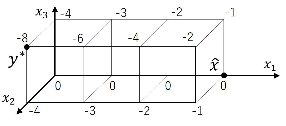
For the problem (SP) with and , itself is an optimal solution. The distance between the unique minimizer of and is , which can be arbitrarily large by taking a sufficiently large . ∎
3 Proofs
3.1 Minimizer Cut Property
We derive Theorem 2.9 from the following variants of the minimizer cut property for s.s. quasi \Mnat-convex functions.
Theorem 3.1.
Let be a function
with (SSQM♮) satisfying ,
and .
(i)
Let and suppose that the minimum of
over
is attained by some .
Then,
there exists some minimizer of satisfying
(ii) Symmetrically to (i), let and suppose that the minimum of over is attained by some . Then, there exists some minimizer of satisfying
(iii)
Suppose that the minimum of
over
is attained by some .
Then,
there exists some minimizer of satisfying
.
(iv)
Symmetrically to (iii),
suppose that the minimum of
over
is attained by some .
Then,
there exists some minimizer of satisfying
.
Proof of Theorem 2.9.
We first consider the case of (i.e., and ). By the choice of , we have . Hence, we can apply Theorem 3.1 (i) (if ) or Theorem 3.1 (iii) (if ) to obtain some such that . If then we are done since satisfies the desired condition (2.3).
We consider the case . Let be the restriction of to . Since , it holds that
We can check easily that satisfies (SSQM♮) and satisfies
Hence, we can apply Theorem 3.1 (ii) to obtain some minimizer of satisfying . This vector satisfies and as desired in (2.3). Note that is a minimizer of because .
The remaining case (i.e., and ) can be treated similarly by using Theorem 3.1 (iv). ∎
We now give a proof of Theorem 3.1.
Proof of Theorem 3.1.
In the following, we give proofs of (i) and (iii); proofs of (ii) and (iv) can be obtained by applying (i) and (iii) to , respectively.
[Proof of (i)] Put . It suffices to show that holds for some . Let be a vector in that maximizes the value . If satisfies , then we are done. Hence, we assume, to the contrary, that , and derive a contradiction.
The condition (SSQM♮) applied to , , and implies that there exists some such that
| (3.1) | |||
| (3.2) | |||
| (3.3) |
Note that holds. Since , we have
| (3.4) |
By the choice of and , we have
| (3.5) |
where . The inequalities (3.4) and (3.5) exclude the possibilities of (3.1) and (3.2), respectively. Therefore, we have (3.3). The former equation in (3.3) implies that is also a minimizer of , a contradiction to the choice of since .
[Proof of (iii)] The proof given below is similar to that for (i). Put . It suffices to show that holds for some . Let be a vector in that maximizes the value . If satisfies , then we are done. Hence, we assume, to the contrary, that , and derive a contradiction.
The condition (SSQM♮) applied to , , and implies that there exists some such that
| (3.6) | |||
| (3.7) | |||
| (3.8) |
Note that holds. Since , we have
| (3.9) |
By the choice of and , we have
| (3.10) |
where . The inequalities (3.9) and (3.10) exclude the possibilities of (3.6) and (3.7), respectively. Therefore, we have (3.8). The former equation in (3.8) implies that is also a minimizer of , a contradiction to the choice of since . ∎
3.2 Domain Reduction Algorithm
To prove Corollary 2.11, we need to explain the general framework of the domain reduction algorithm for minimization of a function with bounded . For a nonempty bounded set , we denote
We define the peeled set of by
The outline of the algorithm is described as follows.
Algorithm DomainReduction
Step 0: Let .
Step 1: Find a vector in the peeled set .
Step 2: If is a minimizer of , then output and stop.
Step 3: Find an axis-orthogonal hyperplane with some and such that
(Case 1) and or
(Case 2) and .
Step 4: Set
and go to Step 1.
The algorithm successfully finds a minimizer of if the following are true in each iteration:
(DR1) the peeled set in Step 1 is nonempty, and
(DR2) there exists a hyperplane satisfying the desired condition in Step 3.
These conditions hold indeed if is an s.s. quasi \Mnat-convex function, as we show later (after Lemma 3.2).
The number of iterations of the algorithm DomainReduction can be analyzed as follows.
Lemma 3.2 (cf. [12, Section 3]).
If the conditions (DR1) and (DR2) are satisfied in each iteration of DomainReduction, then the algorithm terminates in iterations with .
Proof.
We provide a proof for completeness. We first note that the set always contains a minimizer of . For an iteration of the algorithm, we say that it is of type if the hyperplane found in Step 3 is of the form . In an iteration of type , the value decreases by by the choices of the vector in Step 1 and the hyperplane in Step 3. This implies that after iterations of type , we have , i.e., , and therefore an iteration of type never occurs afterwards. Hence, after iterations we have for all , i.e., consists of a single vector, which must be a minimizer of . ∎
We now assume that is an s.s. quasi \Mnat-convex function (i.e., satisfies (SSQM♮)) such that the effective domain of is a bounded \Mnat-convex set, and show that the conditions (DR1) and (DR2) are satisfied in each iteration. The minimizer cut property (Theorem 2.9) guarantees the condition (DR2) for an s.s. quasi \Mnat-convex function. An axis-orthogonal hyperplane satisfying the condition in Step 3 can be found by evaluating function values times.
The condition (DR1), i.e., the nonemptiness of the peeled set , can be shown as follows. We say that a set is an \Mnat-convex set (see, e.g., [8, Section 4.7]) if it satisfies the following exchange axiom:
, , such that
(3.11)
It is known that for an \Mnat-convex set and an integer interval , their intersection is again an \Mnat-convex set if it is nonempty. Hence, the set in each iteration of the algorithm is always an \Mnat-convex set as far as it is nonempty. The following lemma shows that the set is always nonempty.
Lemma 3.3.
For a bounded \Mnat-convex set , the peeled set is nonempty.
Proof.
The proof can be reduced to a similar statement known for an M-convex set (see, e.g., [8] for the definition of M-convex set). First note that a set is an \Mnat-convex set if and only if the set is an M-convex set. For an \Mnat-convex set , the peeled set of the associated M-convex set is nonempty by [12, Theorem 2.4], whereas . Therefore, we have . ∎
4 Concluding Remarks
4.1 Remarks on Minimizer Cut Property
We note that, in addition to Theorem 2.6, \Mnat-convex functions enjoy the following variants of the minimizer cut property, which are similar to, but stronger than, the statements of Theorem 3.1 for s.s. quasi \Mnat-convex functions. The statements in the theorem below can be obtained from the corresponding statements for M-convex functions [12, Theorem 2.2] (see Theorem A.2 (i), (ii) in Appendix).
Theorem 4.1 (cf. [12, Theorem 2.2]).
Let be an \Mnat-convex function with ,
and .
(i)
Let and let be an element in
minimizing the value .
Then, there exists some minimizer of satisfying
(ii) Symmetrically to (i), let and let be an element in minimizing the value . Then, there exists some minimizer of satisfying
(iii) Let be an element in minimizing the value . Then, there exists some minimizer of satisfying
(iv) Symmetrically to (iii), let be an element in minimizing the value . Then, there exists some minimizer of satisfying
It is in order here to dwell on the difference between Theorem 4.1 and Theorem 3.1 by focusing on the statement (i). The statement (i) of Theorem 4.1 for \Mnat-convex functions covers all possible cases of . In contrast, the statement (i) of Theorem 3.1 for s.s. quasi \Mnat-convex functions puts an assumption that attains the minimum, which means that we can obtain no conclusion if the minimum of over is attained uniquely by . Thus, the statement (i) of Theorem 3.1 is strictly weaker than the statement (i) of Theorem 4.1.
We present an example to show that the statements (i) and (iii) of Theorem 4.1 in the case of do not hold for s.s. quasi \Mnat-convex functions.

Example 4.2.
Here is an example to show that the statements (i) and (iii) of Theorem 4.1 in the case of are not true for s.s. quasi \Mnat-convex functions. Consider the function given by444 This function is an adaptation of the one in [11, Example 5.1] to a discrete quasi convex function. The function in [11, Example 5.1] is used in [11] to point out the difference between the weaker versions of (SSQM♮) and (SSQ\Mnat-EXC-PRJ); see also Section 4.2.
(see Figure 4). Function satisfies the condition (SSQM♮).
For and , minimizes the value among all . However, the unique minimizer does not satisfy , i.e., the statement (i) of Theorem 4.1 does not hold in the case of .
For , minimizes the value among all . However, the unique minimizer does not satisfy , i.e., the statement (iii) of Theorem 4.1 does not hold in the case of . ∎
4.2 Connection with Quasi M-convex Functions
As mentioned in Introduction, the concept of s.s. quasi M-convex function is proposed in [8, 10] as a quasi-convex version of M-convex function. We explain the subtle difference between s.s. quasi M-convexity and s.s. quasi \Mnat-convexity in this section555 The difference between the weaker versions of (SSQM♮) and (SSQ\Mnat-EXC-PRJ) is already pointed out by Murota and Yokoi [11]. .
Recall that the condition (SSQM♮) defining s.s. quasi \Mnat-convexity is obtained by relaxing the condition (\Mnat-EXC) for \Mnat-convex functions. Similarly, the concept of s.s. quasi M-convex function is defined by using the relaxed version of the exchange axiom for M-convex functions as follows.
A function is said to be M-convex if it satisfies the following exchange axiom:
(M-EXC) , , such that
(4.1)
A semi-strictly quasi M-convex function is defined as a function satisfying the following relaxed version of (M-EXC):
(SSQM) , , satisfying at least one of the three conditions:
(4.2) (4.3) (4.4)
Recall also that an \Mnat-convex function is originally defined as the projection of an M-convex function: an \Mnat-convex function is defined as a function such that the function given by
| (4.5) |
is M-convex (i.e., satisfies (M-EXC)). Hence, a function is \Mnat-convex if and only if it satisfies the following exchange axiom obtained by the projection of (M-EXC):
(\Mnat-EXC-PRJ) ,
(i) if , then , satisfying (4.1),
(ii) if , then , satisfying (4.1),
(iii) if , then satisfying (4.1) with .
That is, the following equivalence holds for \Mnat-convex functions.
Theorem 4.3 ([9, Theorem 4.2]).
For ,
| (4.6) |
For s.s. quasi \Mnat-convex functions, we may similarly consider the function in (4.5) and the projected version of (SSQM):
(SSQ\Mnat-EXC-PRJ) ,
(i) if , then , satisfying at least one of (4.2), (4.3), and (4.4),
(ii) if , then , satisfying at least one of (4.2), (4.3), and (4.4),
(iii) if , then satisfying at least one of (4.2), (4.3), and (4.4) with .
While the conditions (\Mnat-EXC-PRJ) and (\Mnat-EXC) are equivalent to each other, as mentioned in Theorem 4.3, the condition (SSQ\Mnat-EXC-PRJ) is not equivalent to, but strictly stronger than, (SSQM♮) for s.s. quasi \Mnat-convex functions. That is, we have
| in (4.5) satisfies (SSQM) satisfies (SSQ\Mnat-EXC-PRJ) satisfies (SSQM♮) | (4.7) |
in contrast to (4.6). To be more specific, it is easy to see that
(SSQ\Mnat-EXC-PRJ) (i) and (ii) together imply (SSQM♮),
(SSQM♮) implies (SSQ\Mnat-EXC-PRJ) (i),
but (SSQM♮) does not imply (ii) and (iii) of (SSQ\Mnat-EXC-PRJ), as shown in the examples below.
Example 4.4.
Consider the function given by
(see Figure 5). Function satisfies the condition (SSQM♮). The condition (SSQ\Mnat-EXC-PRJ) (ii) fails for this function.

Indeed, for , , and , we have a unique element , for which
∎
Example 4.5.
It is known that an s.s. quasi M-convex function (i.e., function satisfying (SSQM)) satisfies the minimizer cut property [10, Theorem 4.3] and the proximity property [10, Theorem 4.4]; it can be shown that an s.s. quasi M-convex function also enjoys the geodesic property (see Section A.2 in Appendix). It follows from this fact that if a function satisfies the (stronger) condition (SSQ\Mnat-EXC-PRJ), then it satisfies the same statements as in Theorem 2.6 (minimizer cut property), Theorem 2.14 (geodesic property), and Theorem 2.17 (proximity property) for \Mnat-convex functions. In this connection we emphasize that the s.s. quasi \Mnat-convex functions in Examples 2.12 and 2.18 do not satisfy (SSQ\Mnat-EXC-PRJ) (iii).
Appendix A Appendix
A.1 Properties on Minimization of M-convex Functions
For ease of comparison between M- and \Mnat-convexity, we recall four theorems for minimization of an M-convex function, which correspond, respectively, to Theorems 2.1, 2.6, 2.14, and 2.17 for an \Mnat-convex function.
Optimality Condition by Local Optimality
Theorem A.1 ([5, Theorem 2.4], [7, Theorem 2.2]).
Let be an M-convex function. A vector is a minimizer of if and only if
The same statement holds also for s.s. quasi M-convex functions [10, Theorem 4.2].
Minimizer Cut Property
Theorem A.2 ([12, Theorem 2.2]).
Let be an M-convex function with ,
and be a vector with .
(i)
For ,
let be an element
minimizing the value .
Then, there exists some minimizer of satisfying
(ii) Symmetrically, for , let be an element minimizing the value . Then, there exists some minimizer of satisfying
(iii) For a pair of distinct elements in minimizing the value , there exists some minimizer of satisfying and .
The same statement holds also for s.s. quasi M-convex functions [10, Theorem 4.3].
Geodesic Property
Theorem A.3 ([14, Corollary 4.2], [3, Theorem 2.4]).
Let be an M-convex function with , and be a vector that is not a minimizer of . Also, let be a pair of distinct elements in minimizing the value , and define
(i)
There exists some that is contained in ;
we have , in particular.
(ii)
It holds that
and .
The same statement holds also for s.s. quasi M-convex functions; see Section A.2 for a proof.
Proximity Property
Theorem A.4 ([4, Theorem 3.4], [10, Theorem 4.4]).
Let be an M-convex function and be an integer. For every vector satisfying
there exists some minimizer of such that .
The same statement holds also for s.s. quasi M-convex functions [10, Theorem 4.4].
A.2 Proof of Geodesic Property for Quasi M-convex Functions
We give a proof for the following geodesic property for semi-strictly quasi M-convex functions.
Theorem A.5.
Let be a function with satisfying (SSQM) (i.e., is semi-strictly quasi M-convex), and be a vector that is not a minimizer of . Also, let be a pair of distinct elements in minimizing the value , and define
(i)
There exists some that is contained in ;
we have , in particular.
(ii)
It holds that
and .
The proof given below is essentially the same as the one in [3] for Theorem A.3 on M-convex functions. In the proof of Theorem A.5 (i) we use the following lemma.
Lemma A.6.
Let be a function with
satisfying (SSQM).
Assume that is not a minimizer of ,
and let be a pair of distinct elements in
minimizing the value .
Define .
(i) For every with ,
there exists some with
such that
.
(ii) For every with ,
there exists some with
such that
.
Proof.
We prove (i) only since (ii) can be proven similarly. We first note that holds since is not a minimizer [10, Theorem 4.2]. By definition, satisfies the condition (SSQM), which, applied to and , implies that there exists some such that at least one of the following conditions holds:
| (A.1) | |||
| (A.2) | |||
| (A.3) |
Note that holds. We have
| (A.4) |
since . By the choice of , we have
| (A.5) |
where . The inequalities (A.4) and (A.5) exclude the possibility of (A.1) and (A.2), respectively. Therefore, we have (A.3). The former equation in (A.3) implies that is also a minimizer of . We also have , which follows from the latter equation in (A.3) and the inequality since . ∎
Proof of Theorem A.5 (i).
Putting , we have . We first show that there exists some such that . Assume, to the contrary, that holds for every . Let be a vector minimizing the value among all such vectors. By Lemma A.6 (i), there exists some with such that . Since , we have . Since and , it follows that . This, however, is a contradiction to the choice of since .
We then show that there exists some satisfying both of and . Let be a vector with . If there exists such with , then we are done. Hence, we assume, to the contrary, that for every with , and suppose that maximizes the value among all such . By Lemma A.6 (ii), there exists some with such that . We show that holds. Since , we have . We also have since . This, however, is a contradiction to the choice of since . Hence, we have .
This concludes the proof of Theorem A.5 (i). ∎
Proof of Theorem A.5 (ii).
We first prove the equation . It holds that
| (A.6) |
where the first inequality is by the triangle inequality. We also have
| (A.7) |
where the first equality is by the inequalities and the second equality is by . The equation follows from (A.6) and (A.7).
We then prove the equation . It follows from , (A.6), and (A.7) that all the inequalities in (A.6) and (A.7) hold with equality; in particular, we have
| (A.8) | |||
| (A.9) |
The equation (A.9) implies that . We can also obtain the reverse inclusion from (A.8). Indeed, for every , we have by , and we also have and since . Hence, holds, implying the equation . ∎
References
- [1] Chen, X., Li, M.: M♮-convexity and its applications in operations. Operations Research 69, 1396–1408 (2021)
- [2] Farooq, R., Shioura, A.: A note on the equivalence between substitutability and M♮-convexity. Pacific Journal of Optimization 1, 243–252 (2005)
- [3] Minamikawa, N., Shioura, A.: Time bounds of basic steepest descent algorithms for M-convex function minimization and related problems. Journal of the Operations Research Society of Japan 64, 45–60 (2021)
- [4] Moriguchi, S., Murota, K., Shioura, A.: Scaling algorithms for M-convex function minimization. IEICE Transactions on Fundamentals of Electronics, Communications and Computer Sciences E85-A, 922–929 (2002)
- [5] Murota, K.: Convexity and Steinitz’s exchange property. Advances in Mathematics 124, 272–311 (1996)
- [6] Murota, K.: Discrete convex analysis. Mathematical Programming 83, 313–371 (1998)
- [7] Murota, K.: Submodular flow problem with a nonseparable cost function. Combinatorica 19, 87–109 (1999)
- [8] Murota, K.: Discrete Convex Analysis. Society for Industrial and Applied Mathematics, Philadelphia (2003)
- [9] Murota, K., Shioura, A.: M-convex function on generalized polymatroid. Mathematics of Operations Research 24, 95–105 (1999)
- [10] Murota, K., Shioura, A.: Quasi M-convex and L-convex functions: quasi-convexity in discrete optimization. Discrete Applied Mathematics 131, 467–494 (2003)
- [11] Murota, K., Yokoi, Y.: On the lattice structure of stable allocations in two-sided discrete-concave market. Mathematics of Operations Research 40, 460–473 (2015)
- [12] Shioura, A.: Minimization of an M-convex function. Discrete Applied Mathematics 84, 215–220 (1998)
- [13] Shioura, A.: Fast scaling algorithms for M-convex function minimization with application to the resource allocation problem. Discrete Applied Mathematics 134, 303–316 (2004)
- [14] Shioura, A.: M-convex function minimization under L1-distance constraint and its application to dock re-allocation in bike sharing system. Mathematics of Operations Research 47, 1566–1611 (2022)
- [15] Tamura, A.: Coordinatewise domain scaling algorithm for M-convex function minimization. Mathematical Programming 102, 339–354 (2005)