This paper was converted on www.awesomepapers.org from LaTeX by an anonymous user.
Want to know more? Visit the Converter page.

Note on approximating the Laplace transform of a Gaussian on a complex disk

Yury Polyanskiy and Yihong Wu Y.P. is with the Department of EECS, MIT, Cambridge, MA, email: [email protected]. Y.W. is with the Department of Statistics and Data Science, Yale University, New Haven, CT, email: [email protected].
Abstract

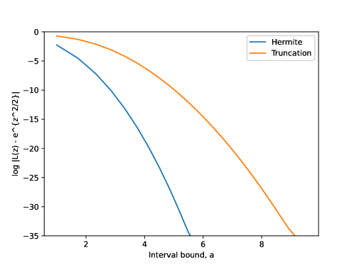
In this short note we study how well a Gaussian distribution can be approximated by distributions supported on [a,a][-a,a]. Perhaps, the natural conjecture is that for large aa the almost optimal choice is given by truncating the Gaussian to [a,a][-a,a]. Indeed, such approximation achieves the optimal rate of eΘ(a2)e^{-\Theta(a^{2})} in terms of the LL_{\infty}-distance between characteristic functions. However, if we consider the LL_{\infty}-distance between Laplace transforms on a complex disk, the optimal rate is eΘ(a2loga)e^{-\Theta(a^{2}\log a)}, while truncation still only attains eΘ(a2)e^{-\Theta(a^{2})}. The optimal rate can be attained by the Gauss-Hermite quadrature. As corollary, we also construct a “super-flat” Gaussian mixture of Θ(a2)\Theta(a^{2}) components with means in [a,a][-a,a] and whose density has all derivatives bounded by eΩ(a2log(a))e^{-\Omega(a^{2}\log(a))} in the O(1)O(1)-neighborhood of the origin.

1 Approximating the Gaussian

We study the best approximation of a Gaussian distribution by compact support measures, in the sense of the uniform approximation of the Laplace transform on a complex disk. Let Lπ(z)=𝑑π(y)ezyL_{\pi}(z)=\int_{\mathbb{R}}d\pi(y)e^{zy} be the Laplace transform, zz\in\mathbb{C}, of the measure π\pi and Ψπ(t)Lπ(it)\Psi_{\pi}(t)\triangleq L_{\pi}(it) be its characteristic function. Denote L0(z)=ez2/2L_{0}(z)=e^{z^{2}/2} and Ψ0(t)=et2/2\Psi_{0}(t)=e^{-t^{2}/2} the Laplace transform and the characteristic function corresponding to the standard Gaussian π0=𝒩(0,1)\pi_{0}=\mathcal{N}(0,1) with density

ϕ(x)1\over2πex2/2,x.\phi(x)\triangleq{1\over\sqrt{2\pi}}e^{-x^{2}/2}\,,\quad x\in\mathbb{R}\,.

How well can a measure π1\pi_{1} with support on [a,a][-a,a] approximate π0\pi_{0}? Perhaps the most natural choice for π1\pi_{1} is the truncated π0\pi_{0}:

π1(dx)ϕa(x)dx,ϕa(x)ϕ(x)\over12Q(a)1{|x|a},\pi_{1}(dx)\triangleq\phi_{a}(x)dx,\qquad\phi_{a}(x)\triangleq{\phi(x)\over 1-2Q(a)}1\{|x|\leq a\}\,, (1)

where Q(a)=[𝒩(0,1)>a]Q(a)=\mathbb{P}[\mathcal{N}(0,1)>a]. Indeed, truncation is asymptotically optimal (as aa\to\infty) in approximating the characteristic function, as made preicse by the following result:

Proposition 1.

There exists some c>0c>0 such that for all a1a\geq 1 and any probability measure π1\pi_{1} supported on [a,a][-a,a] we have

supt|Ψπ1(t)et2/2|ceca2.\sup_{t\in\mathbb{R}}|\Psi_{\pi_{1}}(t)-e^{-t^{2}/2}|\geq ce^{-ca^{2}}\,. (2)

Furthermore, truncation (1) satisfies (for a1a\geq 1)

supt|Ψπ1(t)et2/2|2ea2/2.\sup_{t\in\mathbb{R}}|\Psi_{\pi_{1}}(t)-e^{-t^{2}/2}|\leq 2e^{-a^{2}/2}\,. (3)
Proof.

Let us define B(z)Lπ(z)ez2/2B(z)\triangleq L_{\pi}(z)-e^{z^{2}/2}, a holomorphic (entire) function on \mathbb{C}. Note that if (z)=r\Re(z)=r then

|Lπ(z)|ea|r|,|ez2/2|er2/2,|L_{\pi}(z)|\leq e^{a|r|},\qquad|e^{z^{2}/2}|\leq e^{r^{2}/2}\,,

and thus for r2ar\geq 2a

b(r)sup{|B(z)|:(z)=r}ear+er2/22er2/2b(r)\triangleq\sup\{|B(z)|:\Re(z)=r\}\leq e^{ar}+e^{r^{2}/2}\leq 2e^{r^{2}/2} (4)

On the other hand, for every r3a,a1r\geq 3a,a\geq 1 we have

b(r)|B(r)|er2/2ear1\over2er2/2.b(r)\geq|B(r)|\geq e^{r^{2}/2}-e^{ar}\geq{1\over 2}e^{r^{2}/2}\,. (5)

Applying the Hadamard three-lines theorem to B(z)B(z), we conclude that rlogb(r)r\mapsto\log b(r) is convex and hence

b(3a)(b(0))1/2(b(6a))1/2.b(3a)\leq(b(0))^{1/2}(b(6a))^{1/2}\,. (6)

Since the left-hand side of (2) equals b(0)b(0), (2) then follows from (4)-(6).

For the converse part, in view of (1), the total variation between π0\pi_{0} and its conditional version π1\pi_{1} is given by

|ϕa(x)ϕ(x)|𝑑x=2π0π1TV=2π0([a,a]c)=4Q(a)\int_{\mathbb{R}}|\phi_{a}(x)-\phi(x)|dx=2\|\pi_{0}-\pi_{1}\|_{\rm TV}=2\pi_{0}([-a,a]^{c})=4Q(a)\,

Therefore for the Fourier transform of ϕaϕ\phi_{a}-\phi we get

supt|Ψπ1(t)et2/2|4Q(a)4\over2πaea2/22ea2/2.\sup_{t\in\mathbb{R}}|\Psi_{\pi_{1}}(t)-e^{-t^{2}/2}|\leq 4Q(a)\leq{4\over\sqrt{2\pi}a}e^{-a^{2}/2}\leq 2e^{-a^{2}/2}\,.

Despite this evidence, it turns out that for the purpose of approximating Laplace transform in a neighborhood of 0, there is a much better approximation than (1).

Theorem 2.

There exists some constant c>0c>0 such that for any probability measure π\pi supported on [a,a][-a,a], a1a\geq 1, we have

sup|z|1,z|ez2/2Lπ(z)|ceca2log(a),\sup_{|z|\leq 1,z\in\mathbb{C}}|e^{z^{2}/2}-L_{\pi}(z)|\geq ce^{-ca^{2}\log(a)}\,, (7)

Furthermore, there exists an absolute constant c1>0c_{1}>0 so that for all b1b\geq 1 and all a2c1ba\geq 2c_{1}b there exists distribution π\pi (the Gauss-Hermite quadrature) supported on [a,a][-a,a] such that

sup|z|b,z|ez2/2Lπ(z)|3(c1b/a)a2/4.\sup_{|z|\leq b,z\in\mathbb{C}}|e^{z^{2}/2}-L_{\pi}(z)|\leq 3(c_{1}b/a)^{a^{2}/4}\,.

Taking b=1b=1 implies that the bound (7) is order-optimal.

Remark 1.

When π1\pi_{1} is given by the truncation (1), then performing explicit calculation for zz\in\mathbb{R} we have

Lπ1(z)=ez2/2Φ(a+z)+Φ(az)12Φ(a)1.L_{\pi_{1}}(z)=e^{z^{2}/2}\frac{\Phi(a+z)+\Phi(a-z)-1}{2\Phi(a)-1}\,.

The same expression (by analytic continuation) holds for arbitrary zz\in\mathbb{C} if Φ(z)\Phi(z) is understood as solution of Φ(z)=ϕ(z),Φ(0)=1/2\Phi^{\prime}(z)=\phi(z),\Phi(0)=1/2. For |z|=O(1)|z|=O(1), the approximation error is eΩ(a2)e^{-\Omega(a^{2})}, rather than eΩ(a2loga)e^{-\Omega(a^{2}\log a)}. The suboptimality of truncation is demonstrated on Fig. 1.

Refer to caption
Figure 1: Comparison of approximations of 𝒩(0,1)\mathcal{N}(0,1) by distributions supported on [a,a][-a,a], as measured by the (log of) LL_{\infty} distance between the Laplace transform on the unit disk in \mathbb{C}.
Proof.

As above, denote B(z)=Lπ(z)ez2/2B(z)=L_{\pi}(z)-e^{z^{2}/2}, and define

M(r)=sup|z|r,z|B(z)|.M(r)=\sup_{|z|\leq r,z\in\mathbb{C}}|B(z)|\,.

From (5) we have for any r3a,a1r\geq 3a,a\geq 1

M(r)1\over2er2/2M(r)\geq{1\over 2}e^{r^{2}/2}

and from |Lπ(z)|ea|z||L_{\pi}(z)|\leq e^{a|z|} we also have (for any r2ar\geq 2a):

M(r)ear+er2/22er2/2.M(r)\leq e^{ar}+e^{r^{2}/2}\leq 2e^{r^{2}/2}\,.

Applying the Hadamard three-circles theorem, we have logrlogM(r)\log r\mapsto\log M(r) is convex, and hence

M(3a)(M(1))1λ(M(5a))λ,M(3a)\leq(M(1))^{1-\lambda}(M(5a))^{\lambda}\,,

where λ=log(5a)\overlog(3a)\lambda={\log(5a)\over\log(3a)} and 1λΘ(1\overloga)1-\lambda\Theta({1\over\log a}). From here we obtain for some constant c>0c>0

logM(1)c(a21)log(a),\log M(1)\geq c(-a^{2}-1)\log(a)\,,

which proves (7).

For the upper bound, take π\pi to be the kk-point Gauss-Hermite quadrature of 𝒩(0,1)\mathcal{N}(0,1) (cf. [SB02, Section 3.6]). This is the unique kk-atomic distribution that matches the first 2k12k-1 moments of 𝒩(0,1){\mathcal{N}}(0,1). Specifically, we have:

  • π\pi is supported on the roots of the degree-kk Hermite polynomial, which lie in [4k+2,4k+2][-\sqrt{4k+2},\sqrt{4k+2}] [Sze75, Theorem 6.32];

  • The ii-th moment of π\pi, denoted by mi(π)m_{i}(\pi), satisfies mi(π)=mi(N(0,1))m_{i}(\pi)=m_{i}(N(0,1)) for all i=1,,2k1i=1,\ldots,2k-1.

  • π\pi is symmetric so that all odd moments are zero.

We set k=a2/8k=\lceil a^{2}/8\rceil, so that π\pi is supported on [a,a][-a,a].

Let us denote XπX\sim\pi and G𝒩(0,1)G\sim\mathcal{N}(0,1). By Taylor expansion we get

B(z)=𝔼[ezX]𝔼[ezG]=m=2k1\overm!zm(𝔼[Xm]𝔼[Gm])==k1\over(2)!z2(𝔼[X2]𝔼[G2]).B(z)=\mathbb{E}[e^{zX}]-\mathbb{E}[e^{zG}]=\sum_{m=2k}^{\infty}{1\over m!}z^{m}(\mathbb{E}[X^{m}]-\mathbb{E}[G^{m}])=\sum_{\ell=k}^{\infty}{1\over(2\ell)!}z^{2\ell}(\mathbb{E}[X^{2\ell}]-\mathbb{E}[G^{2\ell}])\,.

Now, we will bound (2)!(2/e)2(2\ell)!\geq(2\ell/e)^{2\ell}, 𝔼[X2]a2\mathbb{E}[X^{2\ell}]\leq a^{2\ell}, 𝔼[G2]=(21)!!(2)\mathbb{E}[G^{2\ell}]=(2\ell-1)!!\leq(2\ell)^{\ell}. This implies that for all |z|b|z|\leq b we have

|B(z)|\displaystyle|B(z)| k{(ea\over2)2+(e\over2)2}|z|2\displaystyle\leq\sum_{\ell\geq k}\left\{\left(ea\over 2\ell\right)^{2\ell}+\left(e\over\sqrt{2\ell}\right)^{2\ell}\right\}|z|^{2\ell}
k{(ea\over2k)2+(e\over2k)2}|z|2\displaystyle\leq\sum_{\ell\geq k}\left\{\left(ea\over 2k\right)^{2\ell}+\left(e\over\sqrt{2k}\right)^{2\ell}\right\}|z|^{2\ell}
2k(c1b/a)2,\displaystyle\leq 2\sum_{\ell\geq k}(c_{1}b/a)^{2\ell}\,,

where in the last step we used ea\over2k,e\over2kc1\overa{ea\over 2k},{e\over\sqrt{2k}}\leq{c_{1}\over a} for some absolute constant c1c_{1}. In all, we have that whenever c1b/a<1/2c_{1}b/a<1/2 we get

|B(z)|2\over1(c1b/a)2(c1b/a)2k3(c1b/a)a2/4.|B(z)|\leq{2\over 1-(c_{1}b/a)^{2}}(c_{1}b/a)^{2k}\leq 3(c_{1}b/a)^{a^{2}/4}\,.

Remark 2.

Note that our proof does not show that for any π\pi supported on [a,a][-a,a], its characteristic function restricted on [1,1][-1,1] must satisfy:

sup|t|1|Ψπ(t)et2/2|ceca2loga.\sup_{|t|\leq 1}|\Psi_{\pi}(t)-e^{-t^{2}/2}|\geq ce^{-ca^{2}\log a}\,.

It is natural to conjecture that this should hold, though.

Remark 3.

Note also that the Gauss-Hermite quadrature considered in the theorem, while essentially optimal on complex disks, is not uniformly better than the naive truncation. For example, due to its finite support, the Gauss-Hermite quadrature is a very bad approximation in the sense of (2). Indeed, for any finite discrete distribution π1\pi_{1} we have lim supt|Ψπ1(t)|=1\limsup_{t\to\infty}|\Psi_{\pi_{1}}(t)|=1, thus only attaining the trivial bound of 11 in the right-hand side of (2). (To see this, note that Ψπ1(t)=j=1kpieitωj\Psi_{\pi_{1}}(t)=\sum_{j=1}^{k}p_{i}e^{it\omega_{j}}. By simultaneous rational approximation (see, e.g., [Cas72, Theorem VI, p. 13]), we have infinitely many values qq such that for all jj |qωj\over2πpj|<1\overq1/k|q{\omega_{j}\over 2\pi}-p_{j}|<{1\over q^{1/k}} for some pjp_{j}\in\mathbb{Z}. In turn, this implies that lim inftmaxj=1,,m(tωjmod2π)=0\liminf_{t\to\infty}\max_{j=1,\ldots,m}(t\omega_{j}\mod 2\pi)=0, and that Ψπ1(t)1\Psi_{\pi_{1}}(t)\to 1 along the subsequence of tt attaining lim inf\liminf.)

2 Super-flat Gaussian mixtures

As a corollary of construction in the previous section we can also derive a curious discrete distribution π2=mwmδxm\pi_{2}=\sum_{m}w_{m}\delta_{x_{m}} supported on [a,a][-a,a] such that its convolution with the Gaussian kernel π2ϕ\pi_{2}*\phi is maximally flat near the origin. More precisely, we have the following result.

Corollary 3.

There exist constants C1,C>0C_{1},C>0 such that for every a>0a>0 there exists k=Θ(a2)k=\Theta(a^{2}), wm0w_{m}\geq 0 with m=1kwm=1\sum_{m=1}^{k}w_{m}=1 and xm[a,a]x_{m}\in[-a,a], m{1,,k}m\in\{1,\ldots,k\}, such that

|(d\overdz)nm=1kwmϕ(zxm)|n!C1eCa2log(a)z,|z|1,n{1,2,}.\left|\left({d\over dz}\right)^{n}\sum_{m=1}^{k}w_{m}\phi(z-x_{m})\right|\leq n!\cdot C_{1}e^{-Ca^{2}\log(a)}\qquad\forall z\in\mathbb{C},|z|\leq 1,n\in\{1,2,\ldots\}\,.
Proof.

Consider the distribution π=m=1kw~mδxm\pi=\sum_{m=1}^{k}\widetilde{w}_{m}\delta_{x_{m}} claimed by Theorem 2 for b=2b=2. Then (here and below CC designates some absolute constant, possibly different in every occurence) we have

sup|z|2|Lπ(z)ez2/2|CeCa2log(a).\sup_{|z|\leq 2}|L_{\pi}(z)-e^{z^{2}/2}|\leq Ce^{-Ca^{2}\log(a)}\,.

Note that the function ez2/2e^{-z^{2}/2} is also bounded on |z|2|z|\leq 2 and thus we have

sup|z|2|Lπ(z)ez2/21|CeCa2log(a).\sup_{|z|\leq 2}|L_{\pi}(z)e^{-z^{2}/2}-1|\leq Ce^{-Ca^{2}\log(a)}\,.

By Cauchy formula, this also implies that derivatives of the two functions inside |||\cdot| must satisfy the same estimate on a smaller disk, i.e.

sup|z|1|(d\overdz)nLπ(z)ez2/2|n!CeCa2log(a).\sup_{|z|\leq 1}\left|\left({d\over dz}\right)^{n}L_{\pi}(z)e^{-z^{2}/2}\right|\leq n!\cdot Ce^{-Ca^{2}\log(a)}\,. (8)

Now, define wm=1\overBw~mexm2/2w_{m}={1\over B}\widetilde{w}_{m}e^{x_{m}^{2}/2}, where B=mw~mexm2/2B=\sum_{m}\widetilde{w}_{m}e^{x_{m}^{2}/2}. We then have an identity:

Lπ(z)ez2/2=Bmwme(zxm)2/2L_{\pi}(z)e^{-z^{2}/2}=B\sum_{m}w_{m}e^{-(z-x_{m})^{2}/2}

Plugging this into (8) and noticing that B1B\geq 1 we get the result. ∎

Remark 4.

This corollary was in fact the main motivation of this note. More exactly, in the study of the properties of non-parametric maximum-likelihood estimation of Gaussian mixtures, we conjectured that certain mixtures must possess some special z0z_{0} in the unit disk on \mathbb{C} such that |mwmϕ(z0xm)|eO(a2)\left|\sum_{m}w_{m}\phi^{\prime}(z_{0}-x_{m})\right|\geq e^{-O(a^{2})}. The stated corollary shows that this is not true for all mixtures. See [PW20, Section 5.3] for more details on why lower-bounding the derivative is important. In particular, one open question is whether the lower bound eO(a2)e^{-O(a^{2})} holds (with high probability) for the case when alogka\asymp\sqrt{\log k} and xm,m{1,,k}x_{m},m\in\{1,\ldots,k\}, are iid samples of 𝒩(0,1)\mathcal{N}(0,1), while wmw_{m}’s can be chosen arbitrarily given xmx_{m}’s.

References

  • [Cas72] J. W. S. Cassels. An Introduction to Diophantine Approximation. Cambridge University Press, Cambridge, United Kingdom, 1972.
  • [PW20] Yury Polyanskiy and Yihong Wu. Self-regularizing property of nonparametric maximum likelihood estimator in mixture models. Arxiv preprint arXiv:2008.08244, Aug 2020.
  • [SB02] J. Stoer and R. Bulirsch. Introduction to Numerical Analysis. Springer-Verlag, New York, NY, 3rd edition, 2002.
  • [Sze75] G. Szegö. Orthogonal polynomials. American Mathematical Society, Providence, RI, 4th edition, 1975.