Not All Noises Are Created Equally:
Diffusion Noise Selection and Optimization
Abstract
Diffusion models that can generate high-quality data from randomly sampled Gaussian noises have become the mainstream generative method in both academia and industry. Are randomly sampled Gaussian noises equally good for diffusion models? While a large body of works tried to understand and improve diffusion models, previous works overlooked the possibility to select or optimize the sampled noise the possibility of selecting or optimizing sampled noises for improving diffusion models. In this paper, we mainly made three contributions. First, we report that not all noises are created equally for diffusion models. We are the first to hypothesize and empirically observe that the generation quality of diffusion models significantly depend on the noise inversion stability. This naturally provides us a noise selection method according to the inversion stability. Second, we further propose a novel noise optimization method that actively enhances the inversion stability of arbitrary given noises. Our method is the first one that works on noise space to generally improve generated results without fine-tuning diffusion models. Third, our extensive experiments demonstrate that the proposed noise selection and noise optimization methods both significantly improve representative diffusion models, such as SDXL and SDXL-turbo, in terms of human preference and other objective evaluation metrics. For example, the human preference winning rates of noise selection and noise optimization over the baselines can be up to 57% and 72.5%, respectively, on DrawBench.
1 Introduction
Generative diffusion models, renowned for the impressive performance (Dhariwal and Nichol,, 2021), serve as the mainstream generative paradigm with wide applications in image generation (Nichol et al.,, 2021; Zhang et al.,, 2023; Saharia et al.,, 2022), image editing (Qi et al.,, 2023; Kawar et al.,, 2023), 3D generation (Gupta et al.,, 2023; Erkoç et al.,, 2023), and video generation (Ho et al., 2022a, ; Ho et al., 2022c, ). Diffusion-based Generative AI products attracted much attention and a large number users in recent years. Understanding and improving the capabilities of diffusion models has become an essentially important topic in machine learning.
A large body of works (Song et al.,, 2020; Fang et al.,, 2023; Podell et al.,, 2023; Sauer et al.,, 2023; Ho et al., 2022b, ; Lin et al.,, 2024) tried to enhance the generated results by working on model weight and architecture space. The importance of noise space is largely overlooked by previous studies, while it is known that diffusion models can generate diverse results, which, of course, contain good ones and bad ones. However, existing works suggest random noises are equal and fail to explore how the noises affect the quality of generated results.
In this work, we try to visit two fundamental issues on noise space of diffusion models. First, is it possible to select better noise according to some quantitative metric? Second, is it possible to optimize a given noise (rather than the model weights) to generate better results? Both answers are affirmative. Fortunately, we not only confirm the possibility but also propose practical algorithms.

Contributions. We summarize the three main contributions of this work as follows:
First, we are the first to hypothesize and empirically verify that not all noises are created equally. Specifically, random noises with high inversion stability usually lead to better generation than noises with lower inversion stability, where the inversion stability can be quantitatively given by the cosine similarity of the sampled noise and the inverse noise . This quantitative metric naturally provides us with a novel noise selection method to select stable noises (e.g. the seed with the highest inversion stability among 100 noise seeds), which often correspond to better generated results. We present several qualitative results of noise selection in Figures 1 and 4.
Second, we further proposed a novel noise optimization method that actively enhances the inversion stability of arbitrary given noises. More specifically, we optimize an inversion-stability loss via gradient descent with respect to the sampled noise (rather than the convention model weight space). The proposed noise optimization method is the first one that works on noise space rather than model weight space to improve diffusion models. We present several qualitative results of noise optimization in Figures 1 and 6.
Third, our extensive experiments demonstrate that the proposed noise selection and noise optimization methods both significantly improve representative diffusion models, such as SDXL and SDXL-turbo. On one hand, the human preference winning rates of noise selection and noise optimization over the baseline can be up to and , respectively, on DrawBench in terms of human preference. On the other hand, noise selection and noise optimization are also preferred by Human Preference Score (HPS) v2 (Wu et al., 2023b, ), the latest state-of-the-art human preference model trained on diverse high-quality human preference data, with winning rates up to and , respectively. Human preference, regarded as the ground-truth ultimate evaluation metric for text-to-image generation, and objective evaluation metrics generally support our methods.
2 Prerequisites
In this section, we formally introduce prerequisites and notations.
Notations. Suppose a diffusion model can generate a clean sample based on some condition , such as a text prompt, given a sampled random noise .111For simplicity, we abuse the latent space and the original data space in the presence of latent diffusion. We denote the score neural network as , the model weights as , the noisy sample at the -th step as , and as the total number of denoising steps.
Diffusion Models. The diffusion models (Ho et al.,, 2020) typically denoise a Gaussian noise along a reverse diffusion path (steps: ) to generate an image step by step. The probability via , denoted as , represents the sampling probability given the previous step’s data. The starting point sampled from a Gaussian distribution, . The probability of the whole chain, , is shown as follows:
| (1) |
where , . The and are the pre-defined parameters for scheduling the scales of adding noises. The is an additional sampling noise at the -th step.
Noise Inversion. The noise inversion is to invert a clean data into a noise along a pre-defined diffusion path. We can write the DDIM inversion process (Hertz et al.,, 2022) as
| (2) |
where people approximate the denoising score prediction at with the inversion score prediction at . Equation (1) can gradually transform a sampled noise into a generated sample along the denoising path, and Equation (2) can gradually transform a generated sample back to a noise along the noise inversion path. We note that the standard noising path which adds independent Gaussian noises is essentially different from the noise inversion path which adds the predicted noise of the score neural network . While the generation denoising path and the noise inversion path are both guided by the score neural network , the sampled noise and the inverse noise are close but not identical due to the cumulative numerical differences.
Fixed Points. We denote the denoising-inversion transformation, , as the transformation function . If and are ideally identical, namely , we call a fixed point of this mapping function . In this case, the inverse noise can perfectly recover the sample generated from . This suggests that a state can remain fixed under some transformation. The fixed points have various great properties and many important applications in various fields, such as projective geometry (Coxeter,, 1998), Nash Equilibrium (Nash Jr,, 1950), and Phase Transition (Wilson,, 1971).
3 Methodology
In this section, we first introduce the noise inversion stability hypothesis and show how it naturally leads to two novel noise-space algorithms, including noise selection and noise optimization.

Noise Inversion Stability. It is well known that fixed points are stable under the transformation and, thus, have great properties (Burton,, 2003; Connell,, 1959; Pata et al.,, 2019). May the fixed-point Gaussian noises under the denoising-inversion transformation also exhibit some advantages? As finding the fixed points of this complex dynamical system is intractable, unfortunately, we cannot empirically verify it. Instead, we can formulate Definition 1 to measure the stability of noise for the denoising-inversion transformation .
Definition 1 (Noise Inversion Stability).
Suppose a sampled noise has its inverse noise for the denoising-inversion transformation given by a diffusion model with the condition . We define the noise inversion stability of the sampled noise as
| (3) |
for the diffusion with the condition , where is the cosine similarity between two vectors.
We use cosine similarity to measure stability for simplicity, while it is also possible to use other similarity metrics. Our empirical analysis in Section 4 suggests that the simple cosine similarity metric works well.
Noise Selection. Inspired by the intriguing mathematical properties of fixed points, we hypothesize that the noise with higher inversion stability can lead to better generated results. If this hypothesis is reasonable, this naturally provides a novel and useful noise selection algorithm that selects the noise seed with the highest stability score from noise seeds (e.g. in this work). We present the pseudocode in Algorithm 1.
Noise Optimization. As we have an objective to increase the noise inversion stability, is it possible to actively optimize a given noise by maximizing the stability score? We further propose the noise optimization algorithm that directly performs Gradient Descent (GD) on the loss, , with respect to , where we keep the diffusion model weights and constant for each optimization step. We present the illustration of noise optimization in the right column of Figure 2. We present the pseudocode in Algorithm 2.
4 Empirical Analysis
In this section, we conduct extensive experiments to demonstrate the effectiveness of our methods. We take text-to-image generation as our main setting.
4.1 Experimental Settings
Models: SDXL-turbo (Sauer et al.,, 2023) and SDXL (Podell et al.,, 2023). SDXL is a representative and powerful diffusion model. SDXL-turbo is a recent accelerated diffusion model which can produce results better than standard SDXL but only take 4 denoising steps. We choose the denoising steps for SDXL-turbo as 4 steps and SDXL as 10 steps for reducing computational time and carbon emissions, unless we specify it otherwise. We also empirically study how the proposed methods depend on the denoising steps in Appendix B.
Dataset: We use all 200 test prompts from the DrawBench dataset (Saharia et al.,, 2022) which contain comprehensive and diverse descriptions beyond the scope of the common training data. We use the first 100 test prompts from the Pick-a-Pic (Kirstain et al.,, 2024) which consist of interesting prompts gathered from the users of the Pick-a-Pic web application. In case studies on color, style, text rendering, object co-occurrence, position, and counting, we specifically collected some prompts from the GenEval dataset (Ghosh et al.,, 2024).
Evaluation metrics: We evaluate the quality of the generated images using both human preference and popular objective evaluation metrics, including HPS v2 (Wu et al., 2023b, ), AES (Schuhmann et al.,, 2022), PickScore (Kirstain et al.,, 2024), and ImageReward (Xu et al.,, 2024). AES indicates a conventional aesthetic score for images, while HPS v2, PickScore, and ImageReward are all emerging human reward models that approximate human preference for text-to-image generation. Particularly, HPS v2 is the state-of-the-art human reward model so far and offers a metric more close to human preference (see Table 6 in (Wu et al., 2023b, )) than other objective evaluation metrics. Moreover, human preference is regarded as the ground-truth and ultimate evaluation method for text-to-image generation. Thus, we regard human preference and HPS v2 as the two most important metrics.
Hyperparameters: For the noise selection experiments, we select the (most) stable noise and the (most) unstable noise from 100 noise seeds according the noise inversion stability. We evaluate generated results using human preference and objective evaluation metrics. For the noise optimization experiments, we initialize the noise using one random seed and perform GD to optimize the noise with 100 steps. The default values of the learning rate and the momentum are 100 and 0.5, respectively.
4.2 The Experiments of Noise Selection
| Dataset | Noise | HPS v2 | AES | PickScore | ImageReward | Average |
|---|---|---|---|---|---|---|
| Pick-a-Pic | Unstable noise | 27.2688 | 5.9265 | 21.6227 | 0.7812 | 13.8998 |
| Stable noise | 27.4934 | 5.9960 | 21.6372 | 0.8981 | 14.0062 | |
| DrawBench | Unstable noise | 28.1377 | 5.3945 | 22.4251 | 0.7021 | 14.1646 |
| Stable noise | 28.4266 | 5.6082 | 22.4200 | 0.7325 | 14.2968 |

The noise selection experiments are to compare the results denoised from stable noises and unstable noises, where the noise with the highest stability score is the stable noise and the noise with the lowest stability score score is defined as unstable noise.
Quantitative results. We present the objective evaluation scores in Table 1. The HPS v2 is the main objective evaluation metric, as it is the state-of-the-art human reward model. The HPS v2 score of stable noises surpasses it counterpart of unstable noise by 0.225 and 0.289, respectively, on Pick-a-Pic and DrawBench. The average scores also support the advantage of stable noises over unstable noises. The quantitative results supports the noise inversion stability hypothesis and suggest that stable noises often significantly outperform unstable noises in practice.
Besides the scores, the winning rates can tell the percentage of one result better than the other on the evaluated prompts. We particularly show the winning rates of human preference and and HPS v2 in Figure 3 to visualize two representative evaluation metrics. All winning rates are significantly higher than 50%. The human preference winning rates are higher than 56%. The HPS v2 winning rates are even up to 65% and 67% over Pick-a-Pic and DrawBench.
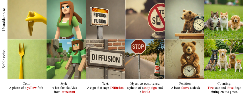
Qualitative results. We conduct case studies for qualitative comparison. We not only care about the standard visual quality, but also further focus on those challenging cases for diffusion models, such as color, style, text rendering, object co-occurrence, position, and counting. The results in Figure 4 show that the images denoised from stable noise are significantly better than images denoised from unstable noise in various aspects. 1) Color: the stable noise leads to a yellow fork accurately, while the unstable noise can only lead to a yellow hand with an incorrect fork. 2) Style: the stable noise obviously correspond to the “Minecraft” style more precisely with rich background details. 3) Text rendering: the stable noise can render the correct “diffusion”. 4) Object co-occurrence, the stable noise can generate correct combinations of two objects, while the unstable noise falsely merges two concepts together. 5) Position, the stable noise correct the wrong position relation of the unstable noises. 6) Counting, the stable noises accurately correct the number of both cats and dogs.
In summary, both quantitative and qualitative results demonstrate the significant effectiveness of noise selection according to the noise inversion stability.
4.3 The Experiments of Noise Optimization
| Dataset | Noise | HPS v2 | AES | PickScore | ImageReward | Average |
|---|---|---|---|---|---|---|
| Pick-a-Pic | Original Noise | 25.9800 | 5.9903 | 21.0183 | 0.2500 | 13.3207 |
| Optimized Noise | 26.6422 | 6.0504 | 21.2344 | 0.4622 | 13.5973 | |
| DrawBech | Original Noise | 26.6203 | 5.4889 | 21.4815 | 0.0575 | 13.4121 |
| Optimized Noise | 27.3651 | 5.5438 | 21.6508 | 0.1767 | 13.6841 |


The noise optimization experiments are to compare the results of original noises and optimized noises. For each prompt, we sample a Gaussian noise as the original noise and learn optimized noises by Algorithm 2. Note that optimized noises are approximately but not real Gaussian noises.
Quantitative results. We present quantitative results in Table 2. All objective evaluation metrics in the experiment consistently support the advantage of optimized noises over original noises. The HPS v2 score of optimized noises surpasses it counterpart of original noises by 0.662 and 0.745, respectively, on Pick-a-Pic and DrawBench. The average score again supports the advantage of optimized noises over original noises.
Similarly, we visualize the winning rates of two most important metrics, HPSv2 and human preference to show the percentage of improved cases in Figure 3. The human preference winning rates of noise optimization are 69% and 72.5%, respectively, over Pick-a-Pic and DrawBench, while the HPS v2 winning rates are even up to 87% and 88%. The winning rate improvements are comparable to the performance gap between two generations of SD models, such as SDXL-turbo (Sauer et al.,, 2023) and cascaded pixel diffusion models (IF-XL) (Saharia et al.,, 2022) .
Qualitative results. We presents the qualitative results of original noises and optimized noises in Figure 6. Similar to what we observe for noise selection, noise optimization also improve multiple challenging cases, such as color, style, text rendering, object co-occurrence, position, and counting we mentioned above. Moreover, we also present the examples that noise optimization can improve the details of human characters and bodies in Figure 7. Optimized noises can lead to more accurate human motion and appearance. For example, the huntress’s hand generated by the optimized noise are accurately holding the end of the arrow.
Robustness to the number of denoising steps . The noise inversion process directly depend on the number of denoising steps . We apply our noise optimization to SDXL with various denoising steps to study the robustness of noise optimization to the hyperparameter . We present the winning rates of noise selection with in Figure 8. The results shows that the improvement of noise optimization is relatively robust to a wide choice of denoising steps. Optimized noises are especially good for very few denoising steps.

Noise Optimization for 3D Generation. It is easy to see that the proposed methods can be generally applied to other diffusion models. Here, we provide an example. We apply noise optimization to 3D generation tasks with a popular image-to-3D generative model, SV3D (Voleti et al.,, 2024). We clearly observe the improvements in body details of these 3D characters. Due to the space limit, we leave more experimental details and results in Appendix C.
In summary, noise optimization can significantly improve generated results in multiple challenging aspects. It is especially surprising that optimized noises deviated from Gaussian noises can help diffusion models generate better results than real Gaussian noises.
5 Discussion and Limitations
In this section, we further discuss related works and the limitations of this work. While this work reports very interesting findings and proposes novel algorithms on noise space of diffusion models, it still has several limitations.
Related Work The noise inversion technique is mainly applied on image editing (Mokady et al.,, 2023; Meiri et al.,, 2023; Huberman-Spiegelglas et al.,, 2023) in very similar ways. They usually invert a clean image into a relatively noisy one via a few inverse steps and then denoise the inverse noisy images with another prompt to achieve instruction editing. Some works (Mao et al.,, 2023) in this line of research realized that editing noises can help editing generated results. Specifically, modifying a portion of the initial noise can affect the layout of the generated images. Other works (Liu et al.,, 2024; Shi et al.,, 2023) focused on dragging and dropping image content via interactive noise editing. However, the goal of previous studies is to control image layout under fine-grained control conditions, such as input layout or editing operations. In contrast, we focus on generally improving generated results of diffusion models by selecting or optimized a Gaussian noise according to the stability score.
Theoretical Understanding. With the inspirations from fixed points in dynamical systems, we still do not theoretically understand why not all noises are created for diffusion models. We formulated and empirically verified the hypothesis that random noises with higher inversion stability often lead to better generated results, it is still difficult to theoretically analyze how the performance of diffusion models mathematically depend on noise stability. We believe theoretically understanding noise selection and noise optimization will be a key step to further improve them.
Optimization Strategies. In this, we only applied simple gradient descent with multiple (e.g., ) steps to optimize the noise-space loss, but noise optimization seems like a difficult optimization task. In some cases, we observe that the loss does not converge smoothly. Due to computational costs and poor understanding towards noise-space loss landscape, we did not carefully fine-tune the hyperparameters or employ advanced optimizers, such as Adam (Kingma and Ba,, 2015) in this work. Thus, our current optimization strategy is far from releasing the power of noise-space algorithms. We think it will be very promising and important to better analyze and solve this emerging optimization task with advanced methods.
Computational Costs. Both noise selection and noise optimization require significantly more computational costs and time than the standard generation. For noise selection, we compute the inversion stability loss of 100 noise seeds and select the one with the highest stability score. Thus, we need to repeat the forward and inversion process for 100 times. For noise optimization, we perform gradient descent with 100 steps. Thus, we need to repeat the forward, inversion and gradient computing process each for 100 times. It may be difficult to specifically accelerate each step of noise selection, but it will be very likely to accelerate noise optimization with less GD steps in near future.
6 Conclusion
In this paper, we report an interesting noise inversion stability hypothesis and empirically observe that noises with higher inversion stability often lead to better generated results. This hypothesis motivates us to design two novel noise-space algorithms, noise selection and noise optimization, for diffusion models. To the best of our knowledge, we are the first to report that not all noises are created equally for diffusion models and the first to generally improve diffusion models without fine-tune the model parameters. Our extensive experiments demonstrate that the proposed methods can significantly improve multiple aspects of qualitative results and enhance human preference rates as well as objective evaluation scores. Moreover, the proposed methods can be generally applied to various diffusion models in a plug-and-play manner. While some limitations exist, our work has made the first solid step to explore this promising direction. We believe our work will motivate more studies on understanding and improving diffusion models from the perspective of noise space.
References
- Burton, (2003) Burton, T. (2003). Stability by fixed point theory or liapunov’s theory: A comparison. Fixed point theory, 4(1):15–32.
- Connell, (1959) Connell, E. H. (1959). Properties of fixed point spaces. Proceedings of the American Mathematical Society, 10(6):974–979.
- Coxeter, (1998) Coxeter, H. S. M. (1998). Non-euclidean geometry. Cambridge University Press.
- Dhariwal and Nichol, (2021) Dhariwal, P. and Nichol, A. (2021). Diffusion models beat gans on image synthesis. Advances in neural information processing systems, 34:8780–8794.
- Erkoç et al., (2023) Erkoç, Z., Ma, F., Shan, Q., Nießner, M., and Dai, A. (2023). Hyperdiffusion: Generating implicit neural fields with weight-space diffusion. In Proceedings of the IEEE/CVF International Conference on Computer Vision, pages 14300–14310.
- Fan et al., (2024) Fan, X., Bhattad, A., and Krishna, R. (2024). Videoshop: Localized semantic video editing with noise-extrapolated diffusion inversion. arXiv preprint arXiv:2403.14617.
- Fang et al., (2023) Fang, G., Ma, X., and Wang, X. (2023). Structural pruning for diffusion models.
- Ghosh et al., (2024) Ghosh, D., Hajishirzi, H., and Schmidt, L. (2024). Geneval: An object-focused framework for evaluating text-to-image alignment. Advances in Neural Information Processing Systems, 36.
- Gupta et al., (2023) Gupta, A., Xiong, W., Nie, Y., Jones, I., and Oğuz, B. (2023). 3dgen: Triplane latent diffusion for textured mesh generation. arXiv preprint arXiv:2303.05371.
- Hertz et al., (2022) Hertz, A., Mokady, R., Tenenbaum, J., Aberman, K., Pritch, Y., and Cohen-Or, D. (2022). Prompt-to-prompt image editing with cross attention control. arXiv preprint arXiv:2208.01626.
- (11) Ho, J., Chan, W., Saharia, C., Whang, J., Gao, R., Gritsenko, A., Kingma, D. P., Poole, B., Norouzi, M., Fleet, D. J., et al. (2022a). Imagen video: High definition video generation with diffusion models. arXiv preprint arXiv:2210.02303.
- Ho et al., (2020) Ho, J., Jain, A., and Abbeel, P. (2020). Denoising diffusion probabilistic models. Advances in neural information processing systems, 33:6840–6851.
- (13) Ho, J., Saharia, C., Chan, W., Fleet, D. J., Norouzi, M., and Salimans, T. (2022b). Cascaded diffusion models for high fidelity image generation. Journal of Machine Learning Research, 23(47):1–33.
- (14) Ho, J., Salimans, T., Gritsenko, A., Chan, W., Norouzi, M., and Fleet, D. J. (2022c). Video diffusion models. Advances in Neural Information Processing Systems, 35:8633–8646.
- Huberman-Spiegelglas et al., (2023) Huberman-Spiegelglas, I., Kulikov, V., and Michaeli, T. (2023). An edit friendly ddpm noise space: Inversion and manipulations. arXiv preprint arXiv:2304.06140.
- Ilharco et al., (2021) Ilharco, G., Wortsman, M., Wightman, R., Gordon, C., Carlini, N., Taori, R., Dave, A., Shankar, V., Namkoong, H., Miller, J., Hajishirzi, H., Farhadi, A., and Schmidt, L. (2021). Openclip. If you use this software, please cite it as below.
- Karras et al., (2022) Karras, T., Aittala, M., Aila, T., and Laine, S. (2022). Elucidating the design space of diffusion-based generative models. Advances in Neural Information Processing Systems, 35:26565–26577.
- Kawar et al., (2023) Kawar, B., Zada, S., Lang, O., Tov, O., Chang, H., Dekel, T., Mosseri, I., and Irani, M. (2023). Imagic: Text-based real image editing with diffusion models. In Proceedings of the IEEE/CVF Conference on Computer Vision and Pattern Recognition, pages 6007–6017.
- Kingma and Ba, (2015) Kingma, D. P. and Ba, J. (2015). Adam: A method for stochastic optimization. 3rd International Conference on Learning Representations, ICLR 2015.
- Kirstain et al., (2024) Kirstain, Y., Polyak, A., Singer, U., Matiana, S., Penna, J., and Levy, O. (2024). Pick-a-pic: An open dataset of user preferences for text-to-image generation. Advances in Neural Information Processing Systems, 36.
- Lin et al., (2024) Lin, S., Wang, A., and Yang, X. (2024). Sdxl-lightning: Progressive adversarial diffusion distillation. arXiv preprint arXiv:2402.13929.
- Liu et al., (2024) Liu, H., Xu, C., Yang, Y., Zeng, L., and He, S. (2024). Drag your noise: Interactive point-based editing via diffusion semantic propagation. arXiv preprint arXiv:2404.01050.
- Mao et al., (2023) Mao, J., Wang, X., and Aizawa, K. (2023). Guided image synthesis via initial image editing in diffusion model. In Proceedings of the 31st ACM International Conference on Multimedia, pages 5321–5329.
- Meiri et al., (2023) Meiri, B., Samuel, D., Darshan, N., Chechik, G., Avidan, S., and Ben-Ari, R. (2023). Fixed-point inversion for text-to-image diffusion models. arXiv preprint arXiv:2312.12540.
- Mokady et al., (2023) Mokady, R., Hertz, A., Aberman, K., Pritch, Y., and Cohen-Or, D. (2023). Null-text inversion for editing real images using guided diffusion models. In Proceedings of the IEEE/CVF Conference on Computer Vision and Pattern Recognition, pages 6038–6047.
- Murray et al., (2012) Murray, N., Marchesotti, L., and Perronnin, F. (2012). Ava: A large-scale database for aesthetic visual analysis. In 2012 IEEE conference on computer vision and pattern recognition, pages 2408–2415. IEEE.
- Nash Jr, (1950) Nash Jr, J. F. (1950). Equilibrium points in n-person games. Proceedings of the national academy of sciences, 36(1):48–49.
- Nichol et al., (2021) Nichol, A., Dhariwal, P., Ramesh, A., Shyam, P., Mishkin, P., McGrew, B., Sutskever, I., and Chen, M. (2021). Glide: Towards photorealistic image generation and editing with text-guided diffusion models. arXiv preprint arXiv:2112.10741.
- Pata et al., (2019) Pata, V. et al. (2019). Fixed point theorems and applications, volume 116. Springer.
- Podell et al., (2023) Podell, D., English, Z., Lacey, K., Blattmann, A., Dockhorn, T., Müller, J., Penna, J., and Rombach, R. (2023). Sdxl: Improving latent diffusion models for high-resolution image synthesis. arXiv preprint arXiv:2307.01952.
- Pressman et al., (2022) Pressman, J. D., Crowson, K., and Contributors, S. C. (2022). Simulacra aesthetic captions. Technical Report Version 1.0, Stability AI. url https://github.com/JD-P/simulacra-aesthetic-captions .
- Qi et al., (2023) Qi, Z., Huang, G., Huang, Z., Guo, Q., Chen, J., Han, J., Wang, J., Zhang, G., Liu, L., Ding, E., et al. (2023). Layered rendering diffusion model for zero-shot guided image synthesis. arXiv preprint arXiv:2311.18435.
- Saharia et al., (2022) Saharia, C., Chan, W., Saxena, S., Li, L., Whang, J., Denton, E. L., Ghasemipour, K., Gontijo Lopes, R., Karagol Ayan, B., Salimans, T., et al. (2022). Photorealistic text-to-image diffusion models with deep language understanding. Advances in neural information processing systems, 35:36479–36494.
- Sauer et al., (2023) Sauer, A., Lorenz, D., Blattmann, A., and Rombach, R. (2023). Adversarial diffusion distillation. arXiv preprint arXiv:2311.17042.
- Schuhmann et al., (2022) Schuhmann, C., Beaumont, R., Vencu, R., Gordon, C., Wightman, R., Cherti, M., Coombes, T., Katta, A., Mullis, C., Wortsman, M., et al. (2022). Laion-5b: An open large-scale dataset for training next generation image-text models. Advances in Neural Information Processing Systems, 35:25278–25294.
- Shi et al., (2023) Shi, Y., Xue, C., Pan, J., Zhang, W., Tan, V. Y., and Bai, S. (2023). Dragdiffusion: Harnessing diffusion models for interactive point-based image editing. arXiv preprint arXiv:2306.14435.
- Song et al., (2020) Song, J., Meng, C., and Ermon, S. (2020). Denoising diffusion implicit models. arXiv preprint arXiv:2010.02502.
- Voleti et al., (2024) Voleti, V., Yao, C.-H., Boss, M., Letts, A., Pankratz, D., Tochilkin, D., Laforte, C., Rombach, R., and Jampani, V. (2024). Sv3d: Novel multi-view synthesis and 3d generation from a single image using latent video diffusion. arXiv preprint arXiv:2403.12008.
- Wang et al., (2004) Wang, Z., Bovik, A. C., Sheikh, H. R., and Simoncelli, E. P. (2004). Image quality assessment: from error visibility to structural similarity. IEEE transactions on image processing, 13(4):600–612.
- Wilson, (1971) Wilson, K. G. (1971). Renormalization group and critical phenomena. i. renormalization group and the kadanoff scaling picture. Physical review B, 4(9):3174.
- (41) Wu, T., Zhang, J., Fu, X., Wang, Y., Ren, J., Pan, L., Wu, W., Yang, L., Wang, J., Qian, C., et al. (2023a). Omniobject3d: Large-vocabulary 3d object dataset for realistic perception, reconstruction and generation. In Proceedings of the IEEE/CVF Conference on Computer Vision and Pattern Recognition, pages 803–814.
- (42) Wu, X., Hao, Y., Sun, K., Chen, Y., Zhu, F., Zhao, R., and Li, H. (2023b). Human preference score v2: A solid benchmark for evaluating human preferences of text-to-image synthesis. arXiv preprint arXiv:2306.09341.
- Xu et al., (2024) Xu, J., Liu, X., Wu, Y., Tong, Y., Li, Q., Ding, M., Tang, J., and Dong, Y. (2024). Imagereward: Learning and evaluating human preferences for text-to-image generation. Advances in Neural Information Processing Systems, 36.
- Zhang et al., (2023) Zhang, L., Rao, A., and Agrawala, M. (2023). Adding conditional control to text-to-image diffusion models. In Proceedings of the IEEE/CVF International Conference on Computer Vision, pages 3836–3847.
- Zhang et al., (2018) Zhang, R., Isola, P., Efros, A. A., Shechtman, E., and Wang, O. (2018). The unreasonable effectiveness of deep features as a perceptual metric. In Proceedings of the IEEE conference on computer vision and pattern recognition, pages 586–595.
Appendix A Experimental Settings of Main Experiments
Computational environment. The experiments are conducted on a computing cluster with GPUs of NVIDIA® Tesla™ A100.
A.1 Datasets and Data Preprocessing
we conduct experiments across three datasets as follows:
Pick-a-Pic. (Kirstain et al.,, 2024): This dataset is composed of data collected from users of the Pick-a-Pic web application. Each example in this dataset consists of a text prompt, a pair of images, and a label indicating the preferred image. It is worth noting that for fast validation and saving computational resources, we only use the first 100 prompts as text conditions to generate images in the main experiment.
DrawBench. (Saharia et al.,, 2022): The examples in this dataset contain a prompt, a pair of images, and two labels for visual quality and prompt alignment. The total number of examples in this dataset is approximately 200. This dataset contains 11 categories of prompts that can be used to test various properties of generated images, such as color, number of objects, text in the scene, etc. The prompts also contain long, complex descriptions, rare words, etc.
GenEval. (Ghosh et al.,, 2024): This dataset contains 553 prompts spanning six attributes, including single object, two objects, counting, colors, positions, and attribute binding. The text prompts are generated from the templates222Templates and prompts are from https://github.com/djghosh13/geneval/tree/main/prompts.
The difference between these datasets: The prompts in Pick-a-Pic are from real users and have more daily descriptions. The prompts in DrawBench have more complex descriptions and contain rare words. The prompts in GenEval are simple but outstanding property descriptions.
In all main experiments, we set all tensor as half precision to improve experimental efficiency. In calculating the inversion stability, we expand the noise tensor to a one-dimensional vector along the channel dimension.
A.2 The Hyperparameters:
Noise Selection. In noise selection experiments, for each prompt, we sample 100 noises using random seeds from 0 to 99. According to the inversion stability score, we select the stable noise among all candidate noises, using the algorithm 1.
Noise Optimization. In noise optimization experiments, for each prompt, we first randomly sample a noise using a random seed selected from 0 to 99. This noise is denoted as original noise. We use algorithm 2 to optimize the original noise with 100 gradient descent steps. We set the defaulted learning rate is 100 and equip it the learning rate with a cosine annealing schedule. The default value of monument is 0.5.
A.3 Evaluation Metrics
Human Preference Score v2 (HPS v2): This score is calculated by a finetuned CLIP333The CLIP version is ViT-H/14 on the HPD v2 dataset (Wu et al., 2023b, ), a comprehensive human preference dataset. This human preference dataset is known for its diversity and representativeness. Each instance in the dataset contains a pair of images with prompt and a label of human preference.
Aesthetic Score (AES): The AES444The Github page: https://github.com/christophschuhmann/improved-aesthetic-predictor is calculated by the Aesthetic Score Predictor (Schuhmann et al.,, 2022), which is designed by adding five MLP layers on top of a frozen CLIP555The CLIP version is ViT-H/14 and only the MLP layers are fine-tuned by a regression loss term on SAC (Pressman et al.,, 2022), LAION-Logos666https://laion.ai/blog/laion-aesthetics/ and AVA (Murray et al.,, 2012) datasets. The score is ranged from 0 to 10. A higher score means the image has better visual quality.
PickScore: This is also a human preference model. The score is calculated by a finetuned CLIP which is trained on the Pick-a-Pic dataset with a large number of user-annotated human preference data samples.
ImageReward: This is an early human preference model (Xu et al.,, 2024).
Human evaluation: Human annotators select a better one from a pair of images following the criteria:
-
•
The correctness of semantic alignment
-
•
The correctness of object appearance and structure
-
•
The richness of details
-
•
The aesthetic appeal of the image
-
•
Your preference for upvoting or sharing it on social networks
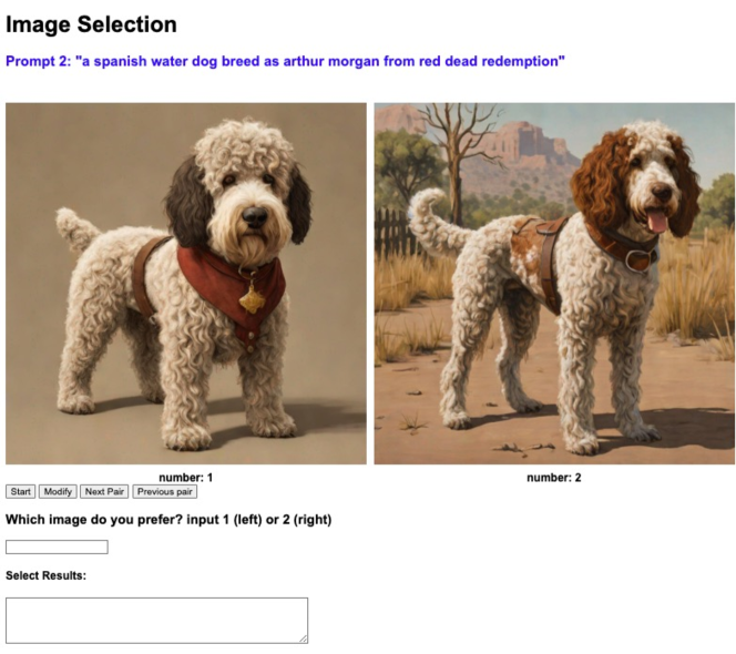
We built a web page for human evaluation, as shown in Figure 10.
The difference between these metrics: The AES is primary for evaluating the visual quality, while others are for human preference.
Appendix B Supplementary Experimental Results
We show more results of noise optimization experiments in Figure 11

Appendix C 3D Object Generation
In this section, we analyze noise optimization for 3D diffusion models.
C.1 Methodology
The noise inversion rule of image-to-3D diffusion models is different from text-to-image diffusion. Here we derive the noise inversion rule for the popular image-to-3D diffusion model, SV3D (Voleti et al.,, 2024).
SV3D employs the EDM framework (Karras et al.,, 2022), which improves upon DDIM with a reparameterized to the denoising process. Taking a single image as input, SV3D generates a multi-view consistent video sequence of the object based on a specified camera trajectory, showcasing remarkable spatio-temporal properties and generalization capabilities. Specifically, we choose the SV3D-U variant, which, during training, consistently conditions on a static trajectory to generate a 21-frame 3D video sequence, with each frame representing a 360/21 degree rotation of the object.
The denoising process within the EDM framework can be written as
| (4) |
| (5) |
We denote as the noise level of the scheduler at the -th time step and denotes the score network. , , , and are coefficients dependent on the noise schedule and the current time step in Euler sampling method. Subsequently, if we intend to achieve noise inversion , we can modify Equation accordingly as
| (6) |
Following previous work (Fan et al.,, 2024; Hertz et al.,, 2022), during the noise inversion process, we have utilized the noise prediction results at to approximate those at .
C.2 Experimental Setting
C.2.1 Datasets
We randomly sample 30 objects from the OmniObject3D Dataset (Wu et al., 2023a, ) and render them using Blender’s Eevee engine. Each object is rendered in a video sequence comprising 84 frames, with the camera rotating 360/84 degrees between each frame. Additionally, we set the ambient lighting to a white background to match the conditions stipulated by SV3D. It is important to note that, as SV3D has not disclosed the rendering details of its test dataset, achieving pixel-level similarity was challenging.
C.2.2 The Hyperparameters
We set the inference steps to 50 with a cfg coefficient of 2.5, following SV3D’s configuration, and utilize the Euler sampling method for denoising. Noise optimization comprises 20 steps using a gradient descent optimizer with a learning rate of 1500 and a momentum of 0.5.
C.3 Performance Evaluation
We mainly use Perceptual Similarity (LPIPS (Zhang et al.,, 2018)), Structural SIMilarity (SSIM (Wang et al.,, 2004)), and CLIP similarity score (CLIP-S (Ilharco et al.,, 2021)) to measure the quality of generated results. Due to the lack of multi-view ground truth, pixel-level evaluation metric, such as PSNR, is not applicable.
The quantitative results in Table 3 demonstrate that optimized noises lead to higher image-to-3D generation quality.
To facilitate a more intuitive comparison, we also present the qualitative results of original noises and optimized noises in Figure 9. It illustrates the significant difference between the optimized noise and the original noise. We can observe that the 3D objects of optimized generally exhibit fewer jagged edges, smoother surfaces, and better fidelity than the results of original noises.
| Model | Noise | LPIPS | SSIM |
|---|---|---|---|
| SV3D-U | Original Noise | 0.2538 | 0.8664 |
| Opti. Noise | 0.2523 | 0.8768 |
Broader Impact
This paper aims at improving diffusion models from the noise-space perspective. While it may have many potential societal consequences, we think none of them must be specifically discussed here.