Norm-in-Norm Loss with Faster Convergence and Better Performance for Image Quality Assessment
Abstract.
Currently, most image quality assessment (IQA) models are supervised by the MAE or MSE loss with empirically slow convergence. It is well-known that normalization can facilitate fast convergence. Therefore, we explore normalization in the design of loss functions for IQA. Specifically, we first normalize the predicted quality scores and the corresponding subjective quality scores. Then, the loss is defined based on the norm of the differences between these normalized values. The resulting “Norm-in-Norm” loss encourages the IQA model to make linear predictions with respect to subjective quality scores. After training, the least squares regression is applied to determine the linear mapping from the predicted quality to the subjective quality. It is shown that the new loss is closely connected with two common IQA performance criteria (PLCC and RMSE). Through theoretical analysis, it is proved that the embedded normalization makes the gradients of the loss function more stable and more predictable, which is conducive to the faster convergence of the IQA model. Furthermore, to experimentally verify the effectiveness of the proposed loss, it is applied to solve a challenging problem: quality assessment of in-the-wild images. Experiments on two relevant datasets (KonIQ-10k and CLIVE) show that, compared to MAE or MSE loss, the new loss enables the IQA model to converge about 10 times faster and the final model achieves better performance. The proposed model also achieves state-of-the-art prediction performance on this challenging problem. For reproducible scientific research, our code is publicly available at https://github.com/lidq92/LinearityIQA.
1. Introduction
Image quality assessment (IQA) has received considerable attention (Wang et al., 2004; Mittal et al., 2012; Ye et al., 2012; Kang et al., 2014; Ma et al., 2016; Hosu et al., 2020) and plays a key role in many vision applications, such as compression (Rippel et al., 2019) and super-resolution (Zhang et al., 2019). It can be achieved by subjective study or objective models. Subjective study uses mean opinion score (MOS) to assess image quality. This is considered as the most reliable and accurate way, whereas it is expensive and time-consuming. So the objective models that can automatically predict image quality are in urgent need. In terms of the availability of the reference image, objective IQA models can be divided into three categories: full-reference IQA (Wang et al., 2004; Zhang et al., 2014; Kim and Lee, 2017; Bosse et al., 2018), reduced-reference IQA (Ma et al., 2011; Xu et al., 2015; Bampis et al., 2017; Liu et al., 2018b), and no-reference IQA (Mittal et al., 2012; Kang et al., 2014; Liu et al., 2017; Ren et al., 2018).
Most classic learning-based IQA models are based on mapping the handcrafted features to image quality by support vector regression (SVR) (Mittal et al., 2012). Recently, deep learning-based models, which jointly learn feature representation and quality prediction, show great promise in IQA (Kang et al., 2014; Ren et al., 2018; Lin and Wang, 2018; Hosu et al., 2020). However, these models mostly treat IQA as a general regression problem. And they adopt standard regression loss functions for training, i.e., mean absolute error (MAE) and mean square error (MSE) between the predicted quality scores and the corresponding subjective quality scores. We notice a fact that the IQA models trained using MAE or MSE loss exhibit slow convergence. For example, on a dataset containing only about 10,000 images with a resolution of 664498, training the model on an NVIDIA GeForce RTX 2080 Ti GPU (11GB) takes more than one day to reach convergence. Since the size of the training dataset becomes larger and larger in the deep learning era, faster convergence is preferable to reduce the training time.
In this work, we tackle the slow convergence problem in the context of IQA. In fact, slow convergence problem is common in machine learning and computer vision, which may be due to the non-smooth loss landscape (Santurkar et al., 2018). To provide faster convergence for the learning process, it is widely-used to do input data normalization or intermediate feature rescaling (Ioffe and Szegedy, 2015; Hoffer et al., 2018). Normalizing the output predictions is rarely recommended. However, it is shown that normalizing the network output can lead to faster convergence of generative networks for image super-resolution (Mullery and Whelan, 2018). Inspired by this work, to achieve fast convergence of IQA model training, we explore normalization in the design of loss functions for IQA.

We propose a class of loss functions, denoted as “Norm-in-Norm”, for training an IQA model with fast convergence. Specifically, the predicted quality scores is firstly subtracted by their mean, and then they are divided by their norm after centralization. Similar normalization is applied to the subjective quality scores. After the normalization, we define the new loss based on the norm of the differences between the normalized values. The new loss normalizes both labels and predictions while label normalization only normalizes labels, and the new loss encourages the IQA model to make linear predictions with respect to (w.r.t.) subjective quality scores. Hence, after training, the linear relationship can be determined by applying least squares regression (LSR) on the whole training set for mapping the predictions to the subjective quality scores. In the testing phase, this learned linear relationship is applied to the model prediction to get the final predicted quality score for a test image.
There are two interesting findings about the new loss. First, we derive that Pearson’s linear correlation coefficient (PLCC)-induced loss (Ma et al., 2018; Liu et al., 2018a) is a special case of the proposed loss, where PLCC is a criterion for benchmarking IQA models. Second, after introducing a variant of the proposed loss, we show its connection to root mean square error (RMSE) — another IQA performance criterion.
Further, we conduct theoretical analysis on the property of the new loss. And it is proved that due to the embedded normalization, the new loss has stronger Lipschitzness and -smoothness (Nesterov, 2013), which means the gradients of the loss function is more stable and more predictable. Thus, the gradient-based algorithm for learning the IQA model has a smoother loss landscape. And this is conducive to the faster convergence of the IQA model.
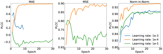
Generally, the proposed “Norm-in-Norm” loss can be applied to any regression problem, including IQA problems. In particular, we pick a challenging real-world IQA problem: quality assessment of in-the-wild images, to verify the effectiveness of the proposed loss. Quality assessment of in-the-wild images has two challenges, i.e., content dependency111Content dependency means human ratings of image quality depend on image content and distortion complexity. We design a no-reference IQA model based on aggregating and fusing multiple level deep features extracted from the image classification network. Deep features are considered for tackling the content dependency. And multiple level features are used for handling the distortion complexity. The model is trained with the proposed loss. The experiments are conducted on two benchmark datasets, i.e., CLIVE (Ghadiyaram and Bovik, 2016) and KonIQ-10k (Hosu et al., 2020). Figure 1 shows the convergence results on KonIQ-10k. By using the proposed loss, the model only needs to look at the training images once (i.e., in one epoch) to achieve a prediction performance indicated by the grey dash line. It is about 10 times faster than MAE loss and MSE loss. This verifies that the proposed loss facilitates faster convergence for training IQA models. We claim that it mainly benefits from the embedded normalization in our loss. Besides the faster convergence, we notice that the proposed loss also leads to a better prediction performance than MAE loss and MSE loss.
To sum up, our main contribution is that we propose a class of normalization-embedded loss functions in the context of IQA. The new loss is shown to have some connections to PLCC and RMSE. And our theoretical analysis proves that the embedded normalization in the proposed loss can facilitate faster convergence. For the quality assessment of in-the-wild images, it is experimentally verified that the new loss can provide both better prediction performance and faster convergence than MAE loss and MSE loss. What’s more, the proposed model outperforms state-of-the-art models on this challenging IQA problem.
2. “Norm-in-Norm” Loss
In this section, we explore the normalization in the design of loss functions, and propose a class of “Norm-in-Norm” loss functions for training IQA models with fast convergence. The idea is to apply normalization for the predicted quality scores and the subjective quality scores respectively using their own statistics when computing the loss.
Assume we have images on the training batch. For the -th image , we denote the predicted quality by an objective IQA model as and its subjective quality score (i.e., MOS) as .
2.1. Loss Computation
Our loss computation can be generally divided into three steps: computation of the statistics, normalization based on the statistics, and loss as the norm of the differences between the normalized values. The left part of Figure 2 shows an illustration of the forward path of the proposed loss. We detail each step in the following.
Computation of the Statistics
First, given the predicted quality scores , we calculate their mean . Similarly, given the subjective quality scores , their mean is calculated. The -norm of the centered values is then computed, respectively.
| (1) | ||||
| (2) |
where is a hyper-parameter. and are the norm of the centered predicted quality scores and the norm of the centered subjective quality scores, respectively.
Normalization Based on the Statistics
Second, we normalize the predicted quality scores and the subjective quality scores based on their own mean and centered norm, respectively. That is, we first subtract the mean from the predicted/subjective quality scores and then divide them by the norm.
| (3) | ||||
| (4) |
where are the normalized predicted quality scores, and are the normalized subjective quality scores.
Loss As the Norm of the Differences
The final step computes the differences between the normalized predicted quality scores and the normalized subjective quality scores . Then the loss is defined as the -th power of the -norm of the differences (), and it is normalized to .
| (5) |
where is a normalization factor. can be determined using Minkowski inequality and Hölder’s inequality (see the Supplementary Materials A), and it follows the following equation.
| (6) |
Based on the forward propagation, we can easily conduct the backward propagation by the chain rule, which is described in the right part of Figure 2.

Specifically, based on Eqn. (3), we have
| (7) |
where is an indicate function, and it equals 1 if , otherwise, 0.
Denote
| (8) |
Then
| (9) |
So we get the derivative of w.r.t. , i.e., .
| (10) |
which includes four terms. The first term is related to . The second term is related to . The thrid term is related to . And the fourth term is related to both and .
Remark: The normalization in Eqn. (3) is invariant to linear predictions. That is, for any , we derive the same . So, we have
| (11) |
The loss encourages the IQA model to make predictions that are linearly correlated with the subjective quality scores.
2.2. A Special Case: PLCC-induced Loss
Pearson’s Linear Correlation Coefficient (PLCC), , is a criterion for benchmarking IQA models, which is defined as follows.
| (12) |
In the following, we will prove that PLCC-induced loss is a special case of the “Norm-in-Norm” loss functions.
First, when is set to 2 in the “Norm-in-Norm” loss, and defined in Eqn. (3-4) relate to the well-known z-score transformation. And and have the following properties.
| (13) |
With the notation of and , we can reformulate PLCC.
When equals to 2, we have using Eqn. (6), then we derive the following equation.
| (14) |
That is, PLCC-induced loss is equivalent to the “Norm-in-Norm” loss when the are all set to 2.
2.3. A Variant and Its Connection to RMSE
In this subsection, we introduce a variant of the “Norm-in-Norm” loss and show its connection to root mean square error (RMSE). In the end of Section 2.1, we remark that the “Norm-in-Norm” loss focuses on training an IQA model to make linear predictions w.r.t. subjective quality scores. Under this linearity assumption, we can only require the normalized predicted quality scores and normalized subjective quality scores to be linearly correlated. That is . With this expectation, we can get a variant of the “Norm-in-Norm” loss as follows.
| (15) |
Connection to RMSE
We apply the least squares regression (LSR) to find the linear mapping between and .
| (16) |
where and are two free parameters.
It is equivalent to solving the following minimization problem.
| (17) | ||||
We substitute into formula (17), and can easily get the minimum loss as follows.
where are considered in our loss variant , and is the centered norm of as defined in Eqn. (2).
Thus, we derive the RMSE between the linearly mapped scores and the subjective quality scores as follows.
| (18) |
That is, a special case of the loss variant with is connected with RMSE — another criterion for benchmarking IQA models.
3. Theoretical Analysis
We introduce the concepts of Lipschitzness and -smoothness (Nesterov, 2013). For a univariate function , is -Lipschitz if . And is -smooth if its gradient is -Lipschitz, i.e., -smoothness corresponds to the Lipschitzness of the gradient. The proposed loss is a differentiate multivariate function w.r.t. the model predictions . Its Lipschitzness is indicated by its gradient magnitude and its -smoothness in the gradient direction is indicated by the quadratic form of its Hessian matrix. Smaller gradient magnitude and quadratic form of its Hessian correspond to better Lipschitzness and -smoothness, respectively.
In this section, we theoretically prove that, when equals 2, the embedded normalization can improve the Lipschitzness and the -smoothness of the proposed loss . That is, the gradient magnitude and the quadratic form of its Hessian are reduced by the embedded normalization, which indicates the gradients of the proposed loss is more stable and more predictable. This ensures that the gradient-based algorithm has a smoother loss landscape, so the training of the IQA model gets more robust and the model converges faster.
First, we prove a theorem about Lipschitzness. When , based on Eqn. (8), . Denote . Thus Eqn. (9) becomes
| (19) |
We show that the gradient magnitude of the new loss satisfies Eqn. (20) in Theorem 3.1 (See proof in Supplemental Materials C).
Theorem 3.1 (Lipschitzness).
When equals 2, the gradient magnitude of the proposed loss has the following property.
| (20) |
where the right side contains three terms. The first term is directly related to the gradient of the loss w.r.t. the normalized predicted quality scores, i.e., . The second term (non-positive) is contributed by . The third term (non-positive) is contributed by . The contributions of and are independent.
The left side of Eqn. (20), , indicates the Lipschitzness with the embedded normalization. Without the normalization, the Lipschitzness is indicated by . From Eqn. (20), we derive that the Lipschitzness of the proposed loss is improved whenever the sum of the gradient deviates from 0 or the gradient correlates the normalized predicted quality scores . In addition, is larger than 1 in practice (see Supplemental Materials B), which also contributes to the improvement of the Lipschitzness. So from Theorem 3.1, we can infer that the embedded normalization improves the Lipschitzness.
Next, we prove a theorem about -smoothness. Denote . We then prove that the quadratic form of the loss Hessian in the gradient direction satisfies Eqn. (3.2) in Theorem 3.2 (The proof is provided in the Supplemental Materials D).
Theorem 3.2 (-smoothness).
When equals 2, the Hessian matrix of the proposed loss has the following property.
| (21) |
Further, when equals 2, we have , where is the identity matrix of order . The above equation becomes
| (22) |
The left side of Eqn. (3.2), , indicates the -smoothness with the embedded normalization. Without the normalization, the -smoothness is indicated by . From Eqn. (3.2), we can see that the -smoothness is improved when the normalized subjective quality scores and normalized predicted quality scores are not linearly correlated (). And it is further improved if the gradient and the normalized predicted quality scores are also not linearly correlated (). In addition, also contributes to the improvement of the -smoothness. So from Theorem 3.2, we can infer that the embedded normalization improves the -smoothness.
4. Verification on Quality Assessment of In-the-Wild Images
Besides theoretical analysis, we also conduct an experimental verification. Quality assessment of in-the-wild images is important for many real-world applications, but few attention is paid to it. In-the-wild images contain lots of unique contents and complex distortions. The greatest challenge for this problem is how to handle the content dependency and distortion complexity. In this section, we pick this challenging problem for verifying the effectiveness of our “Norm-in-Norm” loss in comparison with MAE loss and MSE loss. In addition, we intend to provide state-of-the-art prediction performance on this challenging problem.

4.1. IQA Framework
Our IQA framework for in-the-wild images is shown in Figure 3. We introduce a model that extracts deep pre-trained features for tackling content dependency and fuses multi-level features for handling the distortion complexity. Specifically, it first extracts multi-level deep feature extraction from an image classification backbone (e.g., 32x8d ResNeXt-101 (Xie et al., 2017)). Then feature aggregation is achieved by global average pooling (GAP). Next, features are encoded by an encoder with three fully-connected (FC) layers, where each FC layer is followed by a batch normalization (BN) (Ioffe and Szegedy, 2015) layer and a ReLU activation function. After that, the IQA model concatenates the encoded features from different levels, and the concatenated features are finally mapped to the output by an FC layer. After training the IQA model, to determine the linear mapping from the predictions to the subjective quality scores, the least squares regression (LSR) method is applied on the whole training set. In the testing phase, based on the learned linear mapping, the prediction of the IQA model is linearly mapped to produce the final predicted quality score for a test image.
4.2. Experimental Setup
We conduct experiments on two benchmark datasets: CLIVE (Ghadiyaram and Bovik, 2016) and KonIQ-10k (Hosu et al., 2020). We follow the same experimental setup as described in (Hosu et al., 2020). KonIQ-10k contains 10073 images, and they are divided into three sets: a training set (7058 images), a validation set (1000 images), and a test set (2015 images). We train our model on the training set of KonIQ-10k, save the best performed model on the validation set of KonIQ-10k in terms of Spearman’s Rank-Order Correlation Coefficient (SROCC). We report the SROCC, PLCC, and RMSE values on the test set of KonIQ-10k for prediction performance evaluation. CLIVE includes 1162 images, and it is used for cross-dataset evaluation.
Implementation Details
The input images is resized . The backbone models for multi-level feature extraction are chosen from ResNet-18, ResNet-34, ResNet-50 (He et al., 2016), and ResNeXt-101 (Xie et al., 2017) pre-trained on ImageNet (Deng et al., 2009). And the features are extracted from the stage “conv4” and stage “conv5” of the backbone. To explicitly encode the features at each level to a task-aware feature space, we add auxiliary supervision to the encoded feature at each level. That is, the encoded feature is directly followed by a single FC layer to output the image quality score. Thus, beside the main stream loss, we get another two streams of losses. The final training loss is a weighted average of the three loss values, where the weight hyper-parameters for the main stream loss and the other two streams of losses set to 1, 0.1, 0.1, respectively. We train the model with NVIDIA GeForce RTX 2080 Ti GPU using Adam optimizer for 30 epochs, where the learning rate drops to its 1/10 every 10 epochs. The initial learning rate is chosen from 1e-3, 1e-4, and 1e-5. The batch size varies from 4, 8, 16. And the ratio between the learning rate of the backbone’s parameters and of the other parameters, denoted as “fine-tuned rate”, is selected from 0, 0.01, 0.1, and 1. By default, we use an initial learning rate 1e-4, batch size 8, and fine-tuned rate 0.1. The default values for hyper-parameters and in the “Norm-in-Norm” loss are 1 and 2, respectively. The proposed model is implemented with PyTorch (Paszke et al., 2019). To support reproducible scientific research, we have released our code at https://github.com/lidq92/LinearityIQA.
4.3. Results and Analysis
In this subsection, we show the experimental results and verify the proposed loss in different aspects.
4.3.1. Model Convergence With MAE, MSE, or the Proposed Loss
In this experiment, in the proposed loss are set to , and we adopt the backbone ResNeXt-101 for models trained with all losses. The training/validation/testing curves on KonIQ-10k are shown in Figure 1. Looking at the circle markers, to reach the prediction performance indicated by the grey dash line, MAE and MSE are empirically about ten times slower than the proposed loss. For MAE or MSE loss, to achieve a comparable prediction performance with the proposed loss, the models need to be trained with much more time. And the final state of the convergence also indicates that our proposed loss achieves better prediction performance (higher SROCC/PLCC and lower RMSE) than MAE loss and MSE loss. We experimentally conclude that the model trained with our proposed loss converges faster and better than that with MAE or MSE loss.

Our method may look similar to adding a BN layer to the output of the current model. Thus, our method is also compared with “bnMSE”, where a BN layer is added to the output of the model and the model is trained with MSE loss. Figure 4 shows the validation curves on KonIQ-10k. When compared to MSE, “bnMSE” leads to faster convergence and better performance. However, it is worse than the proposed “Norm-in-Norm”. This is because the learned linear relationship in “bnMSE” is based on the cumulation of the batch-sample statistics, which is not accurate at the beginning. Thus, it will slow down the convergence and somehow disturb the learning process. On the contrast, the proposed method separates the network learning and the learning of the linear relationship, where the network first focuses on making linear predictions and then LSR is applied on the whole training set to determine a more accurate linear relationship. Besides, it should be noted that, unlike “bnMSE”, the proposed method does not change the architecture and it also normalizes subjective quality scores.


| Backbone | , i.e. | |||
|---|---|---|---|---|
| PLCC-induced loss | ||||
| ResNet-18 | 0.916 | 0.918 | 0.912 | 0.913 |
| ResNet-34 | 0.924 | 0.926 | 0.923 | 0.924 |
| ResNet-50 | 0.928 | 0.930 | 0.927 | 0.929 |
| ResNeXt-101 | 0.946 | 0.947 | 0.944 | 0.945 |
4.3.2. Effects of in the “Norm-in-Norm” Loss
In this experiment, we explore the effect of in the proposed loss functions. We consider four choices: , , , and (i.e., PLCC-induced loss). The PLCC values on KonIQ-10k test set for different under different backbones are shown in Table 1. We can see that is generally better than . This can be explained by the fact that the loss with is more sensitive to the outliers than the loss with . Although the loss with is slightly inferior to the loss with , normalization (i.e., ) may improve numerical stability in low-precision implementations as pointed out in (Hoffer et al., 2018). Besides, we now only focus on the task of quality assessment for in-the-wild images, and the results shows that is the best choice for KonIQ-10k. However, the best may be task-dependent and dataset-dependent. It deserves a further study on how to adaptively determine these hyper-parameters in a probability framework, just like the study described in (Barron, 2019).
4.3.3. Training Stability With MAE, MSE, or the Proposed Loss Under Different Learning Hyper-parameters
In this experiment, we consider use ResNet-50 as the backbone model, and vary the default initial learning rate, batch size, and fine-tuned rate to see the training stability under these hyper-parameters. The validation curves on KonIQ-10k are shown in Figure 5. We can see that training models with MAE or MSE loss are unstable when varying the learning rates, batch sizes. And training the model with MAE loss is unstable when fine-tuned rate is too large. Compared to MAE loss and MSE loss, the “Norm-in-Norm” loss is more stable under different choices. For all losses, the best results are achieved under an initial learning rate 1e-4 and a fine-tuned rate 0.1. However, our “Norm-in-Norm” loss can achieve a better validation performance under batch size 16 than under batch size 8, while the MAE or MSE loss does not. This is because our loss is a batch-correlated loss, and a larger batch size may lead to a more accurate estimation of the sample statistics. For fair comparison, in other experiments, we also use the default batch size, i.e., 8, for the proposed loss.


4.3.4. Performance Consistency for MAE, MSE, or the Proposed Loss Among Different Backbone Architectures
In this experiment, we consider ResNet-18, ResNet-34, ResNet-50, and ResNeXt-101 as the backbone architectures, and train the models with MAE, MSE, and the proposed loss. The PLCC on KonIQ-10k test set and the SROCC on CLIVE are shown in Figure 6. It can be seen that our proposed loss consistently achieves the best prediction performance under different backbone architectures. The scatter plots between the predicted quality scores by the models using backbone ResNeXt-101 and MOSs on KonIQ-10k test set are shown in Figure 7. The scatter points of the model with our loss are more centered in the diagonal line, which means a better prediction of image quality.

| Model | Loss | KonIQ-10k | CLIVE | ||
|---|---|---|---|---|---|
| SROCC | PLCC | SROCC | PLCC | ||
| BRISQUE (TIP’12) | SVR loss | 0.705 | 0.707 | 0.561 | 0.598 |
| CORNIA (CVPR’12) | SVR loss | 0.780 | 0.808 | 0.621 | 0.644 |
| HOSA (TIP’16) | SVR loss | 0.805 | 0.828 | 0.628 | 0.668 |
| DeepBIQ (SIViP’18) | SVR loss | 0.872 | 0.886 | 0.742 | 0.747 |
| CNNIQA (CVPR’14) | MAE loss | 0.572 | 0.584 | 0.465 | 0.450 |
| DeepRN (ICME’18) | Huber loss | 0.867 | 0.880 | 0.720 | 0.750 |
| KonCept512 (TIP’20) | MSE loss | 0.921 | 0.937 | 0.825 | 0.848 |
| Proposed | 0.937 | 0.947 | 0.834 | 0.849 | |
| 0.938 | 0.947 | 0.836 | 0.852 | ||
4.4. Performance Comparison with SOTA
In this part, we compare our final model with the state-of-the-art (SOTA) models, i.e., BRISQUE (Mittal et al., 2012), CORNIA (Ye et al., 2012), HOSA (Xu et al., 2016), DeepBIQ (Bianco et al., 2018), CNNIQA (Kang et al., 2014), DeepRN (Varga et al., 2018), and KonCept512 (Hosu et al., 2020). The first three models map handcrafted features to image quality by SVR. The fourth model maps the fine-tuned deep features to image quality by SVR. The last three deep learning-based models adopt MAE, MSE, or their variant Huber loss for network training. And the results of these models are taken from Hosu et al. (2020), while our results are obtained in the same setting. From Table 2, we can see that our model outperforms classic and current deep learning-based models. We note that by combining the loss and its variant with a weight of 1 and 0.1, our model can even achieve better results, e.g., SROCC values are 0.938 and 0.836 on KonIQ-10k test set and CLIVE, respectively.
5. Conclusion
Realizing that most IQA methods train models using MAE or MSE loss with empirically slow convergence, we address this problem by designing a class of loss functions with normalization. The proposed loss includes Pearson correlation-induced loss as a special case. And a special case of the loss variant is connected with RMSE between the linearly mapped predictions and the subjective ratings. We theoretically prove that the embedded normalization helps to improve the smoothness of the loss landscape. Besides, experimental verification of the proposed loss is conducted on the quality assessment of in-the-wild images. Results on two benchmark datasets (KonIQ-10k and CLIVE) show that the model converges faster and better with the proposed loss than that with MAE loss and MSE loss.
The proposed loss is invariant to the scale of subjective ratings. Facilitated with the new loss, we can easily mix multiple datasets with different scales of subjective ratings for training a universal IQA model. In the future study, we intend to verify the effectiveness of this new loss in the universal image and video quality assessment problems. Besides, it is a future direction on how to optimally choose the hyper-parameters and in the class of proposed loss functions for a specific regression task.
Acknowledgements.
This work was partially supported by the National Natural Science Foundation of China under contracts 61572042, 61527804 and 61520106004. We also acknowledge High-Performance Computing Platform of Peking University for providing computational resources.References
- (1)
- Bampis et al. (2017) Christos G Bampis, Praful Gupta, Rajiv Soundararajan, and Alan C Bovik. 2017. SpEED-QA: Spatial efficient entropic differencing for image and video quality. IEEE Signal Processing Letters 24, 9 (2017), 1333–1337.
- Barron (2019) Jonathan T Barron. 2019. A general and adaptive robust loss function. In IEEE Conference on Computer Vision and Pattern Recognition. IEEE, 4331–4339.
- Bianco et al. (2018) Simone Bianco, Luigi Celona, Paolo Napoletano, and Raimondo Schettini. 2018. On the use of deep learning for blind image quality assessment. Signal,Image and Video Processing 12, 2 (2018), 355–362.
- Bosse et al. (2018) Sebastian Bosse, Dominique Maniry, Klaus-Robert Müller, Thomas Wiegand, and Wojciech Samek. 2018. Deep Neural Networks for No-Reference and Full-Reference Image Quality Assessment. IEEE Transactions on Image Processing 27, 1 (2018), 206–219.
- Deng et al. (2009) Jia Deng, Wei Dong, Richard Socher, Li-Jia Li, Kai Li, and Li Fei-Fei. 2009. ImageNet: A large-scale hierarchical image database. In IEEE Conference on Computer Vision and Pattern Recognition. 248–255.
- Ghadiyaram and Bovik (2016) Deepti Ghadiyaram and Alan C. Bovik. 2016. Massive online crowdsourced study of subjective and objective picture quality. IEEE Transactions on Image Processing 25, 1 (2016), 372–387.
- He et al. (2016) Kaiming He, Xiangyu Zhang, Shaoqing Ren, and Jian Sun. 2016. Deep residual learning for image recognition. In IEEE Conference on Computer Vision and Pattern Recognition. 770–778.
- Hoffer et al. (2018) Elad Hoffer, Ron Banner, Itay Golan, and Daniel Soudry. 2018. Norm matters: Efficient and accurate normalization schemes in deep networks. In Advances in Neural Information Processing Systems. 2160–2170.
- Hosu et al. (2020) Vlad Hosu, Hanhe Lin, Tamas Sziranyi, and Dietmar Saupe. 2020. KonIQ-10k: An ecologically valid database for deep learning of blind image quality assessment. IEEE Transactions on Image Processing 29 (2020), 4041–4056.
- Ioffe and Szegedy (2015) Sergey Ioffe and Christian Szegedy. 2015. Batch normalization: Accelerating deep network training by reducing internal covariate shift. In International Conference on Machine Learning. 448–456.
- Kang et al. (2014) Le Kang, Peng Ye, Yi Li, and David Doermann. 2014. Convolutional neural networks for no-reference image quality assessment. In IEEE Conference on Computer Vision and Pattern Recognition. 1733–1740.
- Kim and Lee (2017) Jongyoo Kim and Sanghoon Lee. 2017. Deep learning of human visual sensitivity in image quality assessment framework. In IEEE Conference on Computer Vision and Pattern Recognition. 1676–1684.
- Lin and Wang (2018) Kwan-Yee Lin and Guanxiang Wang. 2018. Hallucinated-IQA: No-reference image quality assessment via adversarial learning. In IEEE Conference on Computer Vision and Pattern Recognition. 732–741.
- Liu et al. (2018a) Wentao Liu, Zhengfang Duanmu, and Zhou Wang. 2018a. End-to-end blind quality assessment of compressed videos using deep neural networks. In ACM International Conference on Multimedia. ACM, 546–554.
- Liu et al. (2017) Xialei Liu, Joost van de Weijer, and Andrew D Bagdanov. 2017. RankIQA: Learning from rankings for no-reference image quality assessment. In IEEE International Conference on Computer Vision. 1040–1049.
- Liu et al. (2018b) Yutao Liu, Guangtao Zhai, Ke Gu, Xianming Liu, Debin Zhao, and Wen Gao. 2018b. Reduced-reference image quality assessment in free-energy principle and sparse representation. IEEE Transactions on Multimedia 20, 2 (2018), 379–391.
- Ma et al. (2018) Kede Ma, Zhengfang Duanmu, and Zhou Wang. 2018. Geometric transformation invariant image quality assessment using convolutional neural networks. In IEEE International Conference on Acoustics, Speech and Signal Processing. 6732–6736.
- Ma et al. (2016) Kede Ma, Qingbo Wu, Zhou Wang, Zhengfang Duanmu, Hongwei Yong, Hongliang Li, and Lei Zhang. 2016. Group MAD competition-a new methodology to compare objective image quality models. In IEEE Conference on Computer Vision and Pattern Recognition. 1664–1673.
- Ma et al. (2011) Lin Ma, Songnan Li, Fan Zhang, and King Ngi Ngan. 2011. Reduced-reference image quality assessment using reorganized DCT-based image representation. IEEE Transactions on Multimedia 13, 4 (2011), 824–829.
- Mittal et al. (2012) Anish Mittal, Anush Krishna Moorthy, and Alan Conrad Bovik. 2012. No-reference image quality assessment in the spatial domain. IEEE Transactions on Image Processing 21, 12 (2012), 4695–4708.
- Mullery and Whelan (2018) Sean Mullery and Paul F Whelan. 2018. Batch normalization in the final layer of generative networks. arXiv preprint arXiv:1805.07389 (2018).
- Nesterov (2013) Yurii Nesterov. 2013. Introductory lectures on convex optimization: A basic course. Springer Science & Business Media.
- Paszke et al. (2019) Adam Paszke, Sam Gross, Francisco Massa, Adam Lerer, James Bradbury, Gregory Chanan, Trevor Killeen, Zeming Lin, Natalia Gimelshein, Luca Antiga, Alban Desmaison, Andreas Kopf, Edward Yang, Zachary DeVito, Martin Raison, Alykhan Tejani, Sasank Chilamkurthy, Benoit Steiner, Lu Fang, Junjie Bai, and Soumith Chintala. 2019. PyTorch: An imperative style, high-performance deep learning library. In Advances in Neural Information Processing Systems. 8024–8035.
- Ren et al. (2018) Hongyu Ren, Diqi Chen, and Yizhou Wang. 2018. RAN4IQA: Restorative adversarial nets for no-reference image quality assessment. In AAAI Conference on Artificial Intelligence. 7308–7314.
- Rippel et al. (2019) Oren Rippel, Sanjay Nair, Carissa Lew, Steve Branson, Alexander G Anderson, and Lubomir Bourdev. 2019. Learned video compression. In IEEE International Conference on Computer Vision. 3454–3463.
- Santurkar et al. (2018) Shibani Santurkar, Dimitris Tsipras, Andrew Ilyas, and Aleksander Madry. 2018. How does batch normalization help optimization?. In Advances in Neural Information Processing Systems. 2483–2493.
- Varga et al. (2018) Domonkos Varga, Dietmar Saupe, and Tamás Szirányi. 2018. DeepRN: A content preserving deep architecture for blind image quality assessment. In International Conference on Quality of Multimedia Experience. 1–6.
- Wang et al. (2004) Zhou Wang, Alan C. Bovik, Hamid R. Sheikh, and Eero P. Simoncelli. 2004. Image quality assessment: From error visibility to structural similarity. IEEE Transactions on Image Processing 13, 4 (2004), 600–612.
- Xie et al. (2017) Saining Xie, Ross Girshick, Piotr Dollár, Zhuowen Tu, and Kaiming He. 2017. Aggregated residual transformations for deep neural networks. In IEEE Conference on Computer Vision and Pattern Recognition. 1492–1500.
- Xu et al. (2016) Jingtao Xu, Peng Ye, Qiaohong Li, Haiqing Du, Yong Liu, and David Doermann. 2016. Blind Image Quality Assessment Based on High Order Statistics Aggregation. IEEE Transactions on Image Processing 25, 9 (2016), 4444–4457.
- Xu et al. (2015) Yong Xu, Delei Liu, Yuhui Quan, and Patrick Le Callet. 2015. Fractal analysis for reduced reference image quality assessment. IEEE Transactions on Image Processing 24, 7 (2015), 2098–2109.
- Ye et al. (2012) Peng Ye, Jayant Kumar, Le Kang, and David Doermann. 2012. Unsupervised feature learning framework for no-reference image quality assessment. In IEEE Conference on Computer Vision and Pattern Recognition. IEEE, 1098–1105.
- Zhang et al. (2014) Lin Zhang, Ying Shen, and Hongyu Li. 2014. VSI: A visual saliency-induced index for perceptual image quality assessment. IEEE Transactions on Image Processing 23, 10 (2014), 4270–4281.
- Zhang et al. (2019) Wenlong Zhang, Yihao Liu, Chao Dong, and Yu Qiao. 2019. RankSRGAN: Generative adversarial networks with ranker for image super-resolution. In IEEE International Conference on Computer Vision. 3096–3105.
Appendix A Derivation of in Eqn. (6)
Lemma A.1.
When , we have the following norm inequality.
| (23) |
Proof.
We will separately prove the left part and the right part.
1. Proof of the left part.
Denote . We have , , and . Then
| (24) |
That is
| (25) |
| (26) |
| (27) |
| (28) |
2. Proof of the right part.
Based on Hölder inequality, we directly get
| (29) |
Applying -th root calculation to the above equation, we derive
| (30) |
In summary, we proof the lemma. ∎
Derivation of in Eqn. (6):
Based on and the Minkowski inequality, we have
| (31) |
Together with the above lemma and , we can derive
| (32) |
Thus
| (33) |
Appendix B Curve in Our Experiment
Figure 8 shows the curve with respect to iteration, and Figure 9 shows the average curve with respect to epoch. We can see that is larger than 1 in practice.


Appendix C Proof of Theorem 3.1 (Lipschitzness)
Proof.
Denote , and based on , Eqn. (19) becomes
| (34) |
Thus
| (35) |
∎
Appendix D Proof of Theorem 3.2 (-smoothness)
Proof.
When equals 2, Eqn. (7) becomes
| (36) |
And based on , we derive the property of as follow.
| (37) |
Denote , and we know . Thus
| (38) |
| (39) |
| (40) |
| (41) |
So
| (42) |
Note that , and we have
| (43) |
Then
| (44) |
That is
| (45) |
Further, when equals 2, we derive . Then
| (46) |
| (47) |
And
| (48) |
Based on the above equation and Theorem 3.1, we have
| (49) |
Use the above four equations to substitute the corresponding parts in Eqn. (45), we can derive the following equation.
| (50) |
∎
Remark: Based on Cauchy inequality, . So . This indicates that the embedded normalization reduces the quadratic form of the loss Hessian. At the meantime, since , does not contribute to the reduction and it is all provided by .
Appendix E Additional Results
E.1. Different Optimizers
Besides Adam, we show additional results with the SGD/Adadelta optimizer. The experimental setting for Table 3 is similar to the experimental setting for Figure 5LABEL:sub@fig:learningrate. We just replaced Adam with SGD or Adadelta. It can be seen that the model performances are very sensitive to the initial learning rates when using the SGD or Adadelta optimizer. Besides, the best initial learning rate is 1e-1 for the proposed loss, 1e-2 for the MAE loss, and 1e-4 for the MSE loss. From Table 3, we can see that the proposed loss is better than the MAE and MSE losses when the SGD or Adadelta optimizer is used and the best initial learning rate is chosen.
| Initial learning rate | MAE loss | MSE loss | Proposed loss |
|---|---|---|---|
| 1e-1 | 0.843/0.780 | Failed/0.069 | 0.931/0.930 |
| 1e-2 | 0.909/0.861 | 0.781/0.690 | 0.916/0.911 |
| 1e-3 | 0.868/0.068 | 0.839/0.701 | 0.899/0.889 |
| 1e-4 | 0.620/0.007 | 0.890/0.739 | 0.868/0.808 |
| 1e-5 | 0.090/0.138 | 0.851/0.458 | 0.770/0.458 |
E.2. Different Architectures
The experimental setting for Table 4 is similar to the experimental setting for Sec. 4.3.4. We just used the non-BN network architecture (AlexNet or VGG-16) instead of the ResNet-based network as the backbone. From Table 4, we can see that the proposed loss is better than the MSE and MSE losses when AlexNet/VGG-16 is used as the backbone. Together with the experiments on ResNet-based backbones, it can be seen that Batch Normalization layers in networks will not affect the superiority new loss.
| Backbone | MAE loss | MSE loss | Proposed loss |
|---|---|---|---|
| AlexNet | 0.788/0.779 | 0.811/0.799 | 0.879/0.886 |
| VGG-16 | 0.840/0.834 | 0.844/0.835 | 0.910/0.913 |
E.3. t-test
In the paper, the results shown in Table 1 and Table 2 were based on the experiments on one train-validation-test split provided by the KonIQ-10k dataset’s owner. However, for performing the t-test to verify whether the performance gains in Table 1 and Table 2 are statistically significant or not, we need several experiments on different train-validation-test splits. We conducted experiments on 10 random splits of CLIVE with the ResNet-18 backbone and performed the t-test for different combinations of p and q, as well as “” and “”. The results show that, in terms of PLCC, (a) “” is significantly better than “” (p-value 0.018) and “” (p-value 0.028), while it is on par with “” (p-value 0.385). (b) “” is slightly (but not significantly) better than “” (p-value 0.172).