Nonparametric Estimation of the Continuous Treatment Effect with Measurement Error
Abstract
We identify the average dose-response function (ADRF) for a continuously valued error contaminated treatment by a weighted conditional expectation. We then estimate the weights nonparametrically by maximising a local generalised empirical likelihood subject to an expanding set of conditional moment equations incorporated into the deconvolution kernels. Thereafter, we construct a deconvolution kernel estimator of ADRF. We derive the asymptotic bias and variance of our ADRF estimator and provide its asymptotic linear expansion, which helps conduct statistical inference. To select our smoothing parameters, we adopt the simulation-extrapolation method and propose a new extrapolation procedure to stabilise the computation. Monte Carlo simulations and a real data study illustrate our method’s practical performance.
keywords:
continuous treatment, deconvolution kernel, measurement error, sieve estimator, simulation-extrapolation method, stabilised weights1 Introduction
Identifying and estimating the causal effect of a treatment or policy from observational studies is of great interest to economics, social science, and public health researchers. There, confounding issues usually exist (i.e. individual characteristics are related to both the treatment selection and the potential outcome), making the causal effect not directly identifiable from the data. Early studies focused on whether an individual receives the treatment or not (e.g. Rosenbaum and Rubin, 1983, 1984; Hahn, 1998; Hirano et al., 2003). More recently, as opposed to such binary treatments, researchers have been investigating the causal effect of a continuously valued treatment, where the effect depends not only on the introduction of the treatment but also on the intensity; see Hirano and Imbens (2004); Galvao and Wang (2015); Kennedy et al. (2017); Fong et al. (2018); Huber et al. (2020); Dong et al. (2021); Ai et al. (2021, 2022), and Huang et al. (2021), among others. However, all these methods require the treatment data to be measured without errors.
In many empirical applications, the treatment and confounding variables may be inaccurately observed. For example, Mahajan (2006) studied the binary treatment effect when the observed treatment indicators are subject to misclassification; see also Lewbel (2007) and Molinari (2008), among others. Battistin and Chesher (2014) investigated the extent to which confounder measurement error affects the analysis of the treatment effect. Continuous treatment variables are also likely to be measured with error in practice. For example, in the Epidemiologic Study Cohort data from the first National Health and Nutrition Examination (NHANES-I) (see Carroll et al., 2006), over 75% of the variance in the fat intake data is made up of measurement error. However, to the best of our knowledge, no existing work has considered the identification and estimation of the causal effect from such error-contaminated continuous treatment data. To bridge this gap in the body of knowledge, we focus on continuous treatment data measured with classical error; that is, instead of observing the received treatment, researchers only observe the sum of the treatment and a random error.
In particular, we study a causal parameter of primary interest to scholars in the literature, the average dose-response function (ADRF). It is defined as the population mean of the individual potential outcome corresponding to certain levels of the treatment. To resolve the confounding problem, we adopt the most widely imposed assumption in the literature on treatment effects, the unconfoundedness condition (e.g. Rosenbaum and Rubin, 1983, 1984; Hirano and Imbens, 2004), which assumes that the assignment of the treatment is independent of the potential outcome of interest given a set of observable covariates.
Perhaps, the most straightforward approach to this problem is based on some parametric model specifying how the outcome relates to confounders and the treatment. Then one may apply the parametric methods to measurement error data in the literature (see e.g. Carroll et al., 2006). However, the parametric approach suffers from the model misspecification problem and does not incorporate available information on the treatment mechanism. Thus, this paper focuses on robust nonparametric estimation of ADRF.
In the literature on error-free continuous treatment data, nonparametric estimation of ADRF under unconfoundedness assumption has been extensively studied. For example, Galvao and Wang (2015) identified the ADRF via an unconditional weighted expectation, with the weighting function being the ratio of two conditional densities of the treatment variable. They estimated these two conditional densities separately and then constructed the estimator for the ADRF. However, it is well known that such a ratio estimator can be unstable owing to its sensitivity to the denominator estimation (Kang and Schafer, 2007). To improve the robustness of estimation, Kennedy et al. (2017) developed a doubly robust estimator for ADRF by regressing a doubly robust mapping on the treatment; see more detailed discussion in Remark 2 of Section 3.1. Ai et al. (2021) identified ADRF via a weighted conditional expectation on the treatment variable, where the weighting function is the ratio of the treatment variable’s marginal density and its conditional density given the confounders. They estimated the weighting function (but not the two densities in the ratio separately) by maximising entropy subject to some moment restrictions that identify the weighting function, then obtained the nonparametric weighted estimator of the ADRF. The idea of estimating the density ratio directly has also been exploited in the literature in (bio)statistics based on parametric modeling (Qin, 1998), semiparametric modeling (Cheng and Chu, 2004), and machine learning with an augmented dataset (Díaz et al., 2021).
However, no existing methods for the error-free treatment data can be easily extended to the error-contaminated treatment data. Indeed, under the unconfoundedness assumption, all those methods depend on estimating a weighting function with the treatment’s conditional density given the confounders in the denominator. Its estimation is a critical step and full of challenges in the presence of measurement error. Although the nonparametric method of estimating the (conditional) density of a variable measured with the classical error has been developed (see e.g. Fan, 1991a, b; Meister, 2006), estimating the density and plugging it into the denominator suffers from the instability issue mentioned above. Such an issue can be even worse when the treatment is measured with errors. Unfortunately, existing techniques of improving the robustness cannot apply to the measurement error data; for example, Ai et al.’s 2021 approach heavily relies on the moment information of a general function of the treatment variable, which is hard to obtain in the presence of measurement error. To our best knowledge, estimating the moment of a general function of a variable measured with errors and its associated theoretical behaviour are challenging problems and remain open in the literature (see Hall and Lahiri, 2008 and our discussion in section 3.1 for more details).
We propose a broad class of novel and robust nonparametric estimators for the ADRF when the treatment data are measured with error. We first represent the ADRF as in Ai et al. (2021), i.e. a weighted expectation of the observed outcome on the treatment variable, where the weighting function is a ratio of the treatment variable’s marginal density and its conditional density given the confounders. Then we propose a novel approach to identify the weighting function with no need to estimate the moment of a general function of the treatment. Specifically, we propose a local empirical likelihood technique that only requires estimating the conditional moment of a general function of the error-free confounders given each fixed value of the treatment. A consistent nonparametric estimator of such a conditional moment can be obtained by using a local constant deconvolution kernel estimator in the literature on errors-in-variables regression; see Fan and Truong (1993); Carroll and Hall (2004); Hall et al. (2007); Delaigle et al. (2009), and Meister (2009), among others. Moreover, by choosing different criterion functions for the local generalised empirical likelihood, the proposed method produces a wide class of weights, including exponential tilting, empirical likelihood and generalised regression as important special cases. Once the weights are consistently estimated, we construct our estimator of the ADRF by estimating the weighted conditional expectation of the observed outcome using another local constant deconvolution kernel estimator.
Based on our identification theorem and the literature on the local constant deconvolution kernel estimator, it is not hard to see the consistency of our estimator. However, the asymptotic behaviour of a local constant deconvolution kernel estimator incorporated with such local generalised empirical likelihood weight has never been investigated. We show the asymptotic bias of our estimator consists of two parts: the one from estimating the weights and the one from estimating the weighted conditional expectation, but it can achieve the same convergence rate as that in the error-free case. The asymptotic variance depends on the type of measurement error. We study the most commonly used two types of measurement errors: the ordinary smooth and the supersmooth ones. The convergence rate of the variance is slower than that in the error-free case but can achieve the optimal rate for the nonparametric estimation in measurement error literature.
Moreover, without imposing additional conditions, it is well known that the explicit expression of the asymptotic variance of the deconvolution kernel for supersmooth error (e.g. Gaussian error) is not derivable; even the exact convergence rate remains unknown. Therefore, it is common to use residual bootstrap methods to make the inference (see e.g. Fan, 1991a; Delaigle et al., 2009, 2015). However, residual bootstrap methods do not work well in our treatment effect framework. We thus provide the asymptotic linear expansion of our ADRF estimator. Based on this, we propose an undersmoothing (pointwise) confidence interval for the ADRF.
A data-driven method to select the bandwidth for a local polynomial deconvolution kernel estimator is challenging. The only method in the literature to our best knowledge is the simulation-extrapolation (SIMEX) method proposed by Delaigle and Hall (2008). However, the linear back-extrapolation method suggested by the authors performed unstably in our numerical studies. We, thus, propose a new local constant extrapolant function. Monte Carlo simulations show that our estimator is stable and outperforms the naive estimator that does not adjust to the measurement error. We also demonstrate the practical value of our estimator by studying the causal effect of fat intake on breast cancer using the Epidemiologic Study Cohort data from NHANES-I (Carroll et al., 2006).
The remainder of the paper is organised as follows. We introduce the basic framework and notations in Section 2. Section 3 presents our estimation procedure, followed by the asymptotic studies of our estimator in Section 4. We discuss the method of selecting our smoothing parameters in Section 5. Finally, we present our simulation results and real data analysis in Section 6.
2 Basic Framework
We consider a continuously valued treatment in which the observed treatment variable is denoted by with the probability density function and support . Let denote the potential outcome if one was treated at level for . In practice, each individual can only receive one treatment level and we only observe the corresponding outcome . We are also given a vector of covariates , with a positive integer, which is related to both and for . Moreover, we consider the situation in which the treatment level is measured with classical error, that is, instead of observing , we observe such that
| (1) |
where is the measurement error, independent of and , and its characteristic function is known; see Remark 1 for the case in which is unknown.
The goal of this paper is to nonparametrically estimate of the unconditional ADRF from an independent and identically distributed (i.i.d.) sample drawn from the joint distribution of .
is never observed simultaneously for all or even on a dense subset of for any individual, but only at a particular level of treatment, . Thus, to identify from the observed data, the following assumption is imposed in most of the treatment effect literature (e.g. rubin1990comment; Kennedy et al., 2017; Ai et al., 2021, 2022; D’Amour et al., 2021).
Assumption 1
We assume
-
(i)
(Unconfoundedness) for all , given , is independent of , that is, ;
-
(ii)
(No Interference) For , the outcome of individual is not affected by the treatment assignments to any other individuals. That is, for any , , where is the potential outcome of individual given the treatment assignments to individual and the others are and , respectively;
-
(iii)
(Consistency) a.s. if ;
-
(iv)
(Positivity) the generalised propensity score satisfies a.s. for all .
Under Assumption 1, for every fixed , can be identified as follows:
| (2) |
where
| (3) |
with and being the density function of and the conditional density of given , respectively. The function is called the stabilised weights in Ai et al. (2021).
If is fully observable and is known, estimating in (2) is reduced to a standard regression problem. For example, can be consistently estimated using the Nadaraya–Watson estimator:
| (4) |
where is a prespecified univariate kernel function such that , is the bandwidth. However, we do not observe but only in (1) and is also unknown in practice. We address these issues in the next section.
Remark 1
The characteristic function of the measurement error may be unknown in some empirical applications. Several methods of consistently estimating it have been proposed in the literature. For example, Diggle and Hall (1993) assumed that the data from the error distribution are observable and proposed estimating from the error data nonparametrically. In some applications, the error-contaminated observations are replicated, and we can estimate the density from these replicates; see Delaigle et al. (2009). When is known up to certain parameters, parametric methods are applicable (e.g. Meister, 2006). Finally, a nonparametric method without using any additional data is also available (e.g. Delaigle and Hall, 2016). Once a consistent estimator of is obtained, our proposed method can be directly applied.
In particular, the assumptions that, (a) the error distribution is known up to certain parameters that are identifiable from some previous studies and (b) repeated error-contaminated data are available, are commonly met in practice. When assumption (a) is satisfied, we can usually obtain -consistent estimators of the parameters and thus a -consistent estimators of uniformly in , where is the sample size of the previous studies. For example, in our real data example in Section 6.3, the error distribution is known up to the variance. Since the convergence rate of our proposed estimator is slower than , the asymptotic behaviour is insensitive to the estimation of provided that . Under assumption (b), we observe
where the ’s are i.i.d.. Note that
Delaigle et al. (2008) proposed to estimate by . They showed that the deconvolution kernel local constant estimator using this and that using asymptotically behave the same under some regularity conditions. Specifically, when is ordinary smooth (as defined in (18)), they require to be sufficiently smooth relative to ’s density. In the contrast, if is supersmooth as in (19), the optimal convergence rate of a deconvolution kernel local constant estimator is logarithmic in , which is so slow that the error incurred by estimating is negligible. This result can be extended to our setting.
3 Estimation Procedure
To overcome the problem that the ’s are not empirically accessible, we apply the deconvolution kernel approach (e.g. Stefanski and Carroll, 1990; Fan and Truong, 1993). This method is often used in nonparametric regression in which the covariates are measured with classical error, as in (1), and the idea is introduced as follows. The density of is the convolution of the densities of and , meaning that , where and are the characteristic functions of and , respectively. We consider with for all . Using the Fourier inversion theorem, if is integrable, we have
| (5) |
This inspired Stefanski and Carroll (1990) to estimate by , where
| (6) |
with the Fourier transform of the kernel , which aims to prevent from becoming unreliably large in its tails.
Based on this idea, Fan and Truong (1993) proposed a consistent errors-in-variables regression estimator by replacing the ’s in (4) with the ’s. In our context, an errors-in-variables estimator of is
| (7) |
Note that , we have
| (8) |
where the last equation comes from the Fourier inversion theorem. Using this property, has the same asymptotic bias as that of , which shrinks to zero as . Then, to verify its consistency to , it suffices to show that its asymptotic variance decays to zero as , using a straightforward extension of the proof in Fan and Truong (1993).
However, the challenge is that is unknown in practice. We next show how to estimate from the error-contaminated data , .
3.1 Estimating
Observing (3), a straightforward way to estimate is to estimate and and then compute the ratio. However, this ratio estimator is sensitive to low values of since small errors in estimating lead to large errors in the ratio estimator (see Ai et al., 2021, 2022 for an example and Appendix A.1.1 in the supplementary file for a detailed illustration). As in the literature of error-free treatment effect, we treat as a whole and estimated directly to mitigate this problem. In paticular, we estimated it nonparametrically from an expanding set of equations, which is closely related to the idea in Ai et al. (2021). However, their method is not applicable to error-contaminated data.
Specifically, when the ’s are fully observable, Ai et al. (2021) found that the moment equation
| (9) |
holds for any integrable function and , and that it identifies . They further estimated the function by maximising a generalised empirical likelihood, subject to the restrictions of the sample version of (9); see LABEL:Remark:AiEstimator in the supplementary file for more details. However, those restrictions are not computable in our context since is not observable, and the nonparametric estimation of the moment for a general function from contaminated data is challenging and its theoretical properties are difficult to derive, if not impossible. For example, Hall and Lahiri (2008) studied the nonparametric estimation of the absolute moment with subject to ordinary smooth error (see the definition (18)) and found that the theoretical behaviour of the estimator differs depending on : if is an even integer, the -consistency is only achievable under a strong condition ; if is an odd integer, the -consistency is achievable if and only if the distribution of the measurement error is sufficiently “rough” in terms of the convergence rate of to zero in its tails; for not a positive integer, -consistency is generally impossible. For other forms of or the involvement of supersmooth error (see the definition (19)), the consistent nonparametric estimation of as well as the corresponding theoretical behaviour are still open problems to our best knowledge.
Thus, to stabilise the estimation of , we derive another expanding set of equations that can identify from the error-contaminated data and avoids estimating . Specifically, instead of estimating the function , we turn to estimate its projection for every fixed , and find that
| (10) |
holds for any integrable function . Although the equation (10) still depends on the unobservable , can be estimated using the deconvolution kernel introduced in (8) from the observable . In the following theorem, we show that the corresponding moment condition can identify the function from for every fixed .
Theorem 3.1
Let be the deconvolution kernel function defined in (6). For every fixed and any integrable function ,
| (11) |
holds if and only if a.s.
The proof is provided in Appendix A.2 in the supplementary file. Theorem 3.1 suggests a way of estimating the weighting function (i.e. solving a sample analogue of (11) for any integrable function , where goes to 0 as the sample size tends to infinity). However, this implies solving an infinite number of equations, which is impossible using a finite sample of observations in practice. To overcome this difficulty, we approximate the infinite-dimensional function space of using a sequence of finite-dimensional sieves. Specifically, let denote the known basis functions with dimension (e.g. the power series, B-splines, or trigonometric polynomials). The function provides approximation sieves that can approximate any suitable functions arbitrarily well as (see Chen, 2007 for a discussion on the sieve approximation). Since the sieve approximates a subspace of the original function space, also satisfies
| (12) |
Equation (12) asymptotically identifies as . We observe that for any increasing and globally concave function ,
| (13) |
solves (12), where is the derivative of , and is a strictly concave function defined by
Indeed, by the first-order condition , we see that (12) holds with . The estimator of is then expected to be defined as the empirical counterpart of (13). Therefore, for every fixed , we propose estimating by
| (14) |
with and
| (15) |
Some of the deconvolution kernel ’s may take negative values, making the objective function not strictly concave in a finite sample. However, as and , and is a strictly concave function. Therefore, with probability approaching one, is strictly concave and uniquely exists. Remark 3 in Section 5 introduces a way of solving this maximisation problem fast and stably from finite samples.
Our estimator has a local generalised empirical likelihood interpretation. To see this, Appendix A.3 shows that is the dual solution to the following local generalised empirical likelihood maximisation problem: for every fixed ,
| (16) |
where is a distance measure from to 1 for , which is continuously differentiable and satisfies that and
Equation (16) aims to minimise some distance measure between the desired weight and the empirical frequencies locally around a small neighbourhood of , subject to the sample analogue of the moment restriction (12).
Since the dual formulation (14) is equivalent to the primal problem (16) and will simplify the following discussions, we shall express the estimator in terms of in the rest of the discussions. In particular, corresponds to exponential tilting (Kitamura and Stutzer, 1997; Imbens et al., 1998; Ai et al., 2022), corresponds to the empirical likelihood (Owen, 2001), corresponds to the continuous updating of the generalised method of moments (Hansen, 1982), and corresponds to the inverse logistic.
Now, replacing in (7) with , we obtain an estimator of :
| (17) |
Remark 2
When is observed without error, Kennedy et al. (2017) propose a doubly-robust estimator for by regressing a pseudo-outcome
onto , i.e. , where is the outcome regression function, and
with being a prespecified kernel function, and are some consistent estimators for and . Kennedy et al. (2017) showed that enjoys double robustness: (i) when both and are consistently estimated and the product of the estimators’ local rates of convergence is sufficiently small, asymptotically behaves the same as the standard local linear estimator of in (2) with known ; (ii) when either or is consistently estimated and the other is misspecified, is still consistent.
This idea can be adapted to the our setup with measurement error (1) by replacing the standard kernel with the deconvolution one. For example, we can define a doubly-robust estimator of by
where
and is some consistent estimator of . Comparing to our proposed estimator in (17), requires additionally a consistent estimator of from the error-contaminated data . Establishing practical estimators (with tuning parameter techniques) and the corresponding theoretical results for this method is beyond the scope of this paper and will be resolved in future work.
4 Large Sample Properties
In this section, we establish the and convergence rates of for every fixed . We then investigate the asymptotic behaviour of the proposed ADRF estimator . Note that (resp. ) is a nonparametric estimator and that its asymptotic behaviour is affected by the asymptotic bias and variance, which are respectively defined as the expectation and variance of the limiting distribution of (resp. ). Based on (8), we will show that the asymptotic biases of the two estimators are the same as their counterparts in the error-free case. That is, they depend on the smoothness of , , and the density of , and the approximation error based on the sieve basis . In particular, the following conditions are required:
Assumption 2
The kernel function is an even function such that and has finite moments of order 3.
Assumption 3
We assume
-
(i)
the support of is a compact subset of . The support of the treatment variable is a compact subset of .
-
(ii)
(Strict Positivity) there exist a positive constant such that , for all .
Assumption 4
(i) The densities , and are third-order continuously differentiable w.r.t. almost surely. (ii) The derivatives of and , denoted by , are integrable almost surely in .
Assumption 5
For every , (i) the function is -times continuously differentiable w.r.t. , where is an integer; (ii) there exist and a positive constant such that .
Assumption 6
(i) For every , the eigenvalues of are bounded away from zero and infinity, and twice differentiable w.r.t. for . (ii) There is a sequence of constants satisfying , such that as , where denotes the Euclidean norm.
Assumption 7
For every , there exist and a positive constant such that , where .
Assumption 8
, and are bounded for some , for all .
Assumption 3 (i) restricts the covariates and the treatment to be bounded. This condition is commonly imposed in the nonparametric regression literature. Assumption 3 (i) can be relaxed if we restrict the tail distributions of and . For example, Chen et al. (2008, Assumption 3) allowed the support of to be the entire Euclidean space but imposed for some .
Assumption 3 (ii) is a strict positivity condition requires every subject having certain chance of receiving every treatment level regardless of covariates. This condition is also imposed in a large body of literature in the absence of measurement error (see e.g. Kennedy et al., 2017, Assumption 2 and D’Amour et al., 2021, Assumption 3), particularly when no restrictions are imposed on the potential outcome distribution. This condition can be relaxed if other smoothness conditions are imposed on the potential outcome distribution (Ma and Wang, 2020), or if different target parameters are considered; for example, Muñoz and Van Der Laan (2012) studied the estimation of a stochastic intervention causal parameter, defined by , based on a weaker positivity condition, i.e. a.e., where is a user specified intervention function. Díaz and van der Laan (2013) studied the estimation of a conditional causal dose-response curve defined by , where is a subset of observed covariates, based on a weaker positivity condition, i.e. a.e., for a user specified weight function . Although Assumption 3 (ii) is not the mildest condition in the literature, we maintain it throughout this paper owing to its technical benefits, especially in the presence of measurement error.
Assumption 4 includes smoothness conditions required for nonparametric estimation. Under Assumption 1, the parameter of interest can be also written as . Note that Assumption 4 (i) implies that is third-order continuously differentiable almost surely. Furthermore, using Leibniz integral rule and Assumption 4 (ii), we have that the target parameter is third-order continuously differentiable.
Assumption 5 (i) is used to control the complexity (measured by the uniform entropy integral) of the function class such that it forms a Donsker class and the empirical process theory can be applied (Van Der Vaart et al., 1996, Corollary 2.7.2). Despite of its stringency, the smoothness condition of this type is commonly adopted in the literature of nonparametric inference, see Chen et al. (2008, Assumption 4 (i)) and Fan et al. (2021, Condition E.1.7).
Assumption 5 (ii) requires the sieve approximation error of to shrink at a polynomial rate. This condition is satisfied for a variety of sieve basis functions. For example, it can be satisfied with if is discrete, and with if is continuous and is a power series or a B-spline, where is the smoothness of the approximand and is the dimension of . Assumption 7 imposes a similar sieve approximation error for .
Assumption 6 (i) rules out near multicollinearity in the approximating basis functions, which is common in the sieve regression literature. Assumption 6 (ii) is satisfied with if is a power series and with if is a B-spline (Newey, 1997). Assumption 8 imposes the boundedness conditions on the moment of the response variable, which are also standard in the errors-in-variables problem (e.g. Fan and Truong, 1993; Delaigle et al., 2009). This condition is needed for deriving the asymptotic distribution of the proposed estimator by applying the Lyapunov central limit theorem.
Depending on the type of the distribution of and decaying rates of and , the asymptotic variance of our estimator differs. This is different from the error-free case. We consider two types of : the ordinary smooth case and supersmooth case, which are standard in the literature of errors-in-variables problem (see e.g. Fan and Truong, 1993, Delaigle et al., 2009, and Meister, 2009, among others, for more details).
An ordinary smooth error of order satisfies
| (18) |
for some constant . A supersmooth error of order satisfies
| (19) |
for some positive constants and some constants and . Examples of ordinary smooth errors include Laplace errors, Gamma errors, and their convolutions. Cauchy errors, Gaussian errors, and their convolutions are supersmooth errors. The order describes the decaying rate of the characteristic function as , which corresponds to the smoothness of the error distribution (e.g. for Cauchy distribution, for Laplace and Gaussian distribution and for Gamma distribution, it relates to both the shape and the scale parameters).
Since in the inverse Fourier transform representation (5), division by appears, it is natural to expect better estimation results for a larger (i.e. a smaller ); indeed, it is found in the literature (see e.g. Fan, 1991b, Fan and Truong, 1993, Delaigle et al., 2009, and Meister, 2009, among others) that for both the ordinary smooth and supersmooth cases, the higher the order is, the harder the deconvolution will be, i.e. the slower the variance of a deconvolution kernel estimator converges. This is an intrinsic difficulty to the nonparametric estimation with errors in variables (Fan and Truong, 1993, Carroll et al., 2006).
Such an influence will be seen in the convergence rate of our estimator in the following theorems.
Depending on the type of the distribution of , we need the following different conditions on to derive the asymptotic variance:
Assumption O (Ordinary Smooth Case): , and .
Assumption S (Supersmooth Case): is support on and bounded.
These assumptions concern the prespecified kernel function and can be satisfied easily. For example, the one whose Fourier transform is satisfies these conditions (e.g. Fan and Truong, 1993 and Delaigle et al., 2009). In the following two sections, we establish the large sample properties of and under the two types of .
4.1 Asymptotics for the Ordinary Smooth Error
To establish the large sample properties of , we first show that the estimated weight function is consistent and compute its convergence rates under both the norm and the norm.
Theorem 4.1
The proof of Theorem 4.1 is presented in Appendix C. The first part of the rates, and , are the rates of the asymptotic bias. and correspond to the asymptotic variance.
We next establish the asymptotic linear expansion and asymptotic normality of . To aid the presentation, we define the following quantities. For , , where
with . The population mean of both and are zero. Let denote the convolution operator, we define
where , with defined in (18), and defined in Assumption 8. Moreover, let and .
Theorem 4.2
The proof of Theorem 4.2 is presented in Appendix D. From the theorem, we see that as long as and are sufficiently smooth or grows sufficiently fast, and decays fast enough, so that , the error arising from the sieve approximation is asymptotically negligible. For example, using the usual trade-off between the squared bias and variance, achieves the optimal convergence rate, , if . In such a case, we require , and if spline basis is used and if a power series is used (The detailed derivation can be found in Appendix A.5).
The convergence rate above is optimal for all possible nonparametric regression estimators when the regressors are measured with ordinary smooth errors showed in Fan and Truong (1993). Note that for error-free local constant estimator, the convergence rates of the asymptotic bias and variance are and , respectively (see e.g. Fan and Gijbels, 1996). Our proposed estimator has the same rate of asymptotic bias as that in the error-free case, but the asymptotic variance is degenerated by , owing to the ordinary smoothness of the error distribution.
In addition to asymptotic normality, we provide in (20) the asymptotic linear expansion of , which can help conduct statistical inference. It is known in the literature on measurement error (see e.g. Delaigle et al., 2015 Appendix C) that the closed-form asymptotic variances and are difficult to estimate. However, using our linear expansion in (20), to estimate the asymptotic variance, we only need consistent estimators of and . For example, and can be estimated respectively using our and , and can be estimated using Liang’s (2000) method. Then, we can construct a pointwise confidence interval for using the undersmoothing technique (see Appendix A.4 for the detailed method and some simulation results). Other confidence intervals based on bias-correction (see e.g. Calonico et al., 2018; takatsu2022debiased) are also possible but require a better estimation of the asymptotic bias and corresponding adjustments of the variance estimation with theoretical justification. That is beyond the scope of this paper and will be resolved in future work.
4.2 Asymptotics for the Supersmooth Error
The next two theorems establish the asymptotic properties of our estimator for the supersmooth case.
Theorem 4.3
The proof of Theorem 4.3 is presented in Appendix C. Comparing these results with those in Theorem 4.1, the asymptotic bias is the same as that in the ordinary smooth case. The rate of the asymptotic variance, however, becomes much slower, which is expected in the errors-in-variables context; see Fan and Truong (1993) and Delaigle et al. (2009).
Theorem 4.4
The proof of Theorem 4.4 is presented in Appendix D. As in the ordinary smooth case, as long as is sufficiently smooth or grows sufficiently fast, and decays fast enough, the sieve approximation error of our estimator is asymptotically negligible and the dominating bias term is the same as that in the ordinary smooth case. The asymptotic variance is affected by the measurement error . The convergence rate of the variance for bandwidth or , , is degenerated by compared to the rate for the error-free case, owing to the supersmoothness of the error distribution.
From the theorem, when and for a constant , one finds that the rate of variance, , is negligible compared to the asymptotic bias, and the convergence rate of is . This result is analogue to that in the literature on nonparametric regression with measurement error (see e.g. Fan, 1991a, a; Fan and Truong, 1993; Delaigle et al., 2015 among others) and it achieves the optimal convergence rate for all possible nonparametric regression estimators when the regressors are measured with supersmooth errors showed in Fan and Truong (1993).
Note that under the case of supersmooth error, an explicit expression and the exact convergence rate of is extremely hard (if not impossible) to derive without additional assumptions. In order to establish the asymptotic distribution of using Lyapunov central limit theorem, a lower bound of the deconvolution kernel’s second moment is required. In particular, we require . This is commonly imposed in the measurement error literature; see Fan (1991a) and Delaigle et al. (2015) among others. Fan (1991a) showed that this lower bound holds under some mild conditions on and (e.g. (19) and Assumption S hold, for for some , and the real part and the imaginary part of satisfy or as ). These assumptions do not exclude the usually-used kernel function defined below Assumption S and error distributions such as Gaussian, Cauchy and Gaussian mixture.
Our explicit asymptotic linear expansion of in (21) is particularly helpful for statistical inference in the supersmooth error case due to the difficulty of deriving an explicit expression of the asymptotic variance. Most of the literature provides only the convergence rate; see Fan and Truong (1993), Meister (2006), and Meister (2009), among others.
5 Select the Smoothing Parameters
In this section, we discuss how to choose the three smoothing parameters , and to calculate our estimator (see (14), (15), and (17)). Before delving into our method, we need some preliminaries.
5.1 Preliminaries
The smoothing parameters in nonparametric regression are usually selected by either minimising certain cross-validation (CV) criteria or minimising an approximation of the asymptotic bias and variance of the estimator.
In nonparametric errors-in-variables regression, as pointed out by Carroll et al. (2006) and Meister (2009), approximating the asymptotic bias and variance of the estimator can be extremely challenging, if not impossible. Unfortunately, the CV criteria are also not computable. To see this, we assume that and in (14) and (15) are given for now and adapt the CV criteria to our context to choose , which would be
| (22) |
where is a weight function that prevents the CV from becoming too large because of the unreliable data points from the tails of the distributions of and denotes the estimator obtained as in (17), but without using the observations from individual . Now, we see that (22) is not computable in errors-in-variables regression problems since the ’s are not observable.
To tackle this problem, Delaigle and Hall (2008) proposed combining the CV and SIMEX methods (e.g. Cook and Stefanski, 1994 and Stefanski and Cook, 1995). Specifically, in the simulation step, we generate two additional sets of contaminated data, namely and , for and with a large number, where the ’s and ’s are i.i.d. as in (1). Now, inserting first the ’s and then the ’s in (14) and (17) instead of the ’s, we obtain respectively and for . The authors then suggested deriving two CV-type bandwidths, and , which minimise and , respectively, where
for , where and are obtained respectively as and , but without using the observations from individual .
The ’s are the contaminated version of the ’s, which is the same role as the ’s play to the ’s and the ’s play to the ’s. Intuitively, we then expect the relationship between and our target bandwidth to be similar to that between and . Thus, the authors proposed an extrapolation step to obtain an estimator of . Specifically, they considered that and used a linear back-extrapolation procedure that, in our context, would give the bandwidth
| (23) |
5.2 Two-step Procedure and Local Constant Extrapolation
In our case, recall that we have two more smoothing parameters, and . We can either extend the SIMEX method to choose three parameters simultaneously or choose and using other methods first and then apply SIMEX to choose . The first option incurs a high computational burden and is unstable in practice. Thus, we adopt the second choice, which leads to a two-step procedure.
Note from Theorems 4.2 and 4.4 that our estimator achieves optimal rate when trades off the rate of the bias and that of the standard deviation . Note also that the plug-in bandwidth for the kernel deconvolution estimator with bandwidth of the density of proposed by Delaigle and Gijbels (2002) minimises the asymptotic MSE of the estimator, whose bias is of rate of and standard deviation . Thus, we should have our . Moreover, to make satisfy all the conditions in our theorems when , we require .
Thus, we first set . Then, to choose , we note from (11) that holds. We propose to choose such that , where the constant minimises the following generalised CV criterion (Craven and Wahba, 1978):
Such a choice of and is not guaranteed to minimise the error of our final estimator . However, with our choice of below, they guarantee the optimal convergence rate of if B-spline basis is used. For the polynomial sieve basis, the smooth parameter defined in Assumption 5 need to be larger than 1 (see Appendix A.5). Moreover, the simulation results showed that this works well (see Section 6 for more discussion).
In the second step, we could simply adopt in (23). However, in our numerical study, the linear back-extrapolation sometimes gave highly unstable results. We expected a larger number of to reduce the variability; for example, Delaigle and Hall (2008) used . However, even with , we still found some unacceptable results, which was somewhat expected, as which extrapolant function should be used in practice is unknown (Carroll et al., 2006, Section 5.3.2). Therefore, we introduce a new extrapolation procedure.
In particular, instead of extrapolating parametrically from and , we suggest approximating the relationship between the ’s and ’s using a local constant estimator (see Fan and Gijbels, 1996), where and with the constants minimise and , respectively, for . Then, we take this approximated relationship as the extrapolant function. Specifically, we choose the bandwidth to be
| (24) |
where is the Gaussian kernel function. The bandwidth here is selected by leave-one-out cross-validation. Local constant estimator has been well studied and widely used, and can work fairly fast and stable. In our simulation study, we found that is sufficiently large to ensure good performance.
Remark 3
Recall from (15) that some of the deconvolution kernel ’s may take negative values, making the maximisation of not strictly concave in finite samples. With , truncating those negative ’s to 0 is a fast and stable way to solve the problem. The simulation performed well.
6 Numerical Properties


6.1 Simulation Settings
Let be i.i.d. uniform random variables supported on and . We consider the following four models in which is generated from a standard normal distribution for models 1 and 4 and from a uniform distribution supported on for models 2 and 3:
-
1.
, , and ( affects and linearly);
-
2.
, , and ( affects nonlinearly and linearly);
-
3.
, , and ( affects linearly but nonlinearly);
-
4.
, , and ( affects and nonlinearly).
For each model, we generate 200 samples of of size 250 or 500, where with either a Laplace random variable with mean 0 and or a mean zero Gaussian random variable with .
For each combination of the model, sample size, and measurement error type, we calculate our estimator in (17). To measure the quality of the estimator, we calculate the integrated squared errors , where are the 10th and 90th quantiles of , respectively.
To highlight the importance of considering the measurement errors in the estimation, we also calculate the naive estimator that ignored the error for each sample. That is, we apply the estimator of Ai et al. (2021, 2022) to our data by replacing the ’s there with the ’s. Specifically, the naive estimator is
| (25) |
where is the standard normal density function and is calculated using (LABEL:AipiEst) (see Ai et al., 2021, 2022 for more details).
Unless otherwise specified, we take the kernel function for the deconvolution kernel method to be the one whose Fourier transform is given by
To illustrate the potential benefit of using our methods over the naive estimator without confounding the effect of the smoothing parameter selectors, we first use the theoretically optimal smoothing parameters for each method. These parameters simultaneously minimise the integrated squared error (ISE) for each method, resulting in the optimal naive estimator (NV) and the proposed conditional moment estimator (CM).
Recall from Section 5.2 that we do not choose and by minimising the estimated ISE of our estimator. To see how much we might lose by doing so, we calculate the estimator with our choice of and and the optimal that minimised the ISE, which is denoted by .
Finally, to assess the performance of our method in practice, we calculate using the smoothing parameters selected from the data using the method in Section 5.2 and denote it by . We take the weight function to be an indicator function that equals 1 when the ’s or ’s are within their 5% to 95% quantiles, and 0 otherwise. We also compute the naive estimator in (25) with the , and selected using the 10-fold CV method, denoted by , to make a comparison.
6.2 Simulation Results
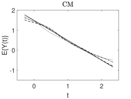
In this section, we show our simulation results. The full simulation results of the 200 values of the ISE of each estimator obtained from the 200 simulated samples for models 1 to 4 can be seen in the boxplots in Appendix A.6. Figures 1 to 3 depict the true curve of the model and three estimated curves corresponding to the 1st, 2nd, and 3rd quartiles of the 200 ISE values.
Overall, the simulation results show that our methods with the theoretically optimal smoothing parameters (CM) perform better than that of the naive one (NV). This confirms the advantages of our methods over the naive one by adapting the estimation to the measurement errors. A graphical example is presented in Figure 1, which shows the quartile curves of NV and CM for models 1 and 2 with Laplace measurement errors and .
The simulation results also confirm our theoretical proportion that the performance of our method improves as the sample size increases. Figure 2 exemplifies the effect of increasing by depicting the quartile curves and ISE boxplots of CM and for model 3 when the measurement errors follow a Laplace distribution with and . The improvement with the increase in sample size can also be seen in the boxplots in the Appendex A.6.
Comparing the ISE values of with those of CM, we find that our choice of and discussed in Section 5.2 lowers the performance of our estimator only marginally in most cases. Recall that is the number of polynomial basis functions of used to estimate and is the bandwidth used to estimate , which are related to the relationship between and as well as that between and . We thus consider the nonlinear relationship between and or between and in the simulation models (see models 2 to 4). Our choice of and still works well compared with the optimal one. Figure 3 provides a graphical example from model 4, where affects both and nonlinearly, with Gaussian measurement errors and .
6.3 Real Data Example
We demonstrate the practical value of our data-driven estimator using Epidemiologic Study Cohort data from NHANES-I. We estimate the causal effect of the long-term log-transformed daily saturated fat intake on the risk of breast cancer based on a sample of 3,145 women aged 25 to 50. The data were analysed by Carroll et al. (2006) using a logistic regression calibration method, and they are available from https://carroll.stat.tamu.edu/data-and-documentation. The daily saturated fat intake was measured using a single 24-hour recall. Specifically, the log-transformation was taken as . Previous nutrition studies have estimated that over 75% of the variance in those data is made up of measurement error. According to Carroll et al. (2006), it is reasonable to assume the classical measurement error model (i.e. (1)), with a Gaussian measurement error on the data. The outcome variable takes 1 if the individual has breast cancer and 0 otherwise. The covariates in are age, the poverty index ratio, the body mass index, alcohol use (yes or no), family history of breast cancer, age at menarche (a dummy variable taking 1 if age is ), menopausal status (pre or post), and race, which are assumed to have been measured without appreciable error.
We first apply our estimator to the data for a Gaussian measurement error with an error variance . That corresponds to . As pointed out by Delaigle and Gijbels (2004), the error variances estimated by other nutrition studies may be inaccurate. Thus, we also consider cases in which , , and (i.e. , and the error-free case).

Figure 4 presents the estimated curves using the smoothing parameters selected as described in section 5 and a 95% undersmoothing pointwise confidence band for (see Appendix A.4 for the method and the confidence bands for and 0.75). Overall, the estimated risk of breast cancer shows a decreasing trend across the range of transformed saturated fat intake. When the measurement error variance is 0.17 of or 0, there is a marginal increasing trend between and 3.4. The 95% confidence bands for and 0.43 show an overall decreasing trend with a slight increase between and 3.4. These findings concur with the results of Carroll et al. (2006), who found in their multivariate logistic regression calibration that the coefficient of the log-transformed saturated fat intake on the risk of breast cancer was significant and negative. However, the results should be treated with extreme caution because of possible misclassification in the breast cancer data and the lack of follow-up of breast cancer cases with high fat intakes; see Carroll et al. (2006, Chap 3.3).
Acknowledgements
The authors would like to sincerely thank the Steffen Lauritzen, the Associate Editor, and the two referees for their constructive suggestions and comments. Wei Huang’s research was supported by the Professor Maurice H. Belz Fund of the University of Melbourne. Zheng Zhang is supported by the fund from the National Natural Science Foundation of China [grant number 12001535], Natural Science Foundation of Beijing [grant number 1222007], and the fund for building world-class universities (disciplines) of Renmin University of China [project number KYGJC2022014]. The authors contributed equally to this work and are listed in the alphabetical order.
References
- Ai et al. (2021) Ai, C., Linton, O., Motegi, K. and Zhang, Z. (2021) A unified framework for efficient estimation of general treatment models. Quantitative Economics, 12, 779–816.
- Ai et al. (2022) Ai, C., Linton, O. and Zhang, Z. (2022) Estimation and inference for the counterfactual distribution and quantile functions in continuous treatment models. Journal of Econometrics, 228, 39–61.
- Battistin and Chesher (2014) Battistin, E. and Chesher, A. (2014) Treatment effect estimation with covariate measurement error. Journal of Econometrics, 178, 707–715.
- Calonico et al. (2018) Calonico, S., Cattaneo, M. D. and Farrell, M. H. (2018) On the effect of bias estimation on coverage accuracy in nonparametric inference. Journal of the American Statistical Association, 113, 767–779.
- Carroll and Hall (2004) Carroll, R. J. and Hall, P. (2004) Low order approximations in deconvolution and regression with errors in variables. Journal of the Royal Statistical Society: Series B (Statistical Methodology), 66, 31–46.
- Carroll et al. (2006) Carroll, R. J., Rupper, D., Stefanski, L. A. and Crainiceanu, C. M. (2006) Measurement Error in Nonlinear Models: A Modern Perspective. Chapman & Hall/CRC.
- Chen (2007) Chen, X. (2007) Large sample sieve estiamtion of semi-nonparametric models. Handbook of Econometrics, 6, 5549–5632.
- Chen et al. (2008) Chen, X., Hong, H. and Tarozzi, A. (2008) Semiparametric efficiency in gmm models with auxiliary data. The Annals of Statistics, 36, 808–843.
- Cheng and Chu (2004) Cheng, K. F. and Chu, C.-K. (2004) Semiparametric density estimation under a two-sample density ratio model. Bernoulli, 10, 583–604.
- Cook and Stefanski (1994) Cook, J. and Stefanski, L. (1994) Simulation-extrapolation estimation in parametric measurement error models. Journal of the American Statistical Association, 89, 1314–1328.
- Craven and Wahba (1978) Craven, P. and Wahba, G. (1978) Smoothing noisy data with spline functions. Numerische Mathematik, 31, 377–403.
- Delaigle et al. (2009) Delaigle, A., Fan, J. and Carroll, R. J. (2009) A design-adaptive local polynomial estimator for the errors-in-variables problem. Journal of the American Statistical Association, 104, 348–359.
- Delaigle and Gijbels (2002) Delaigle, A. and Gijbels, I. (2002) Estimation of integrated squared density derivatives from a contaminated sample. Journal of Royal Statistical Society: Series B (Statistical Methodology), 64, 869–886.
- Delaigle and Gijbels (2004) — (2004) Bootstrap bandwidth selection in kernel density estimation from a contaminated sample. Annals of the Institute of Statistical Mathematics, 56, 19–47.
- Delaigle and Hall (2008) Delaigle, A. and Hall, P. (2008) Using simex for smoothing-parameter choice in errors-in-variables problems. Journal of the American Statistical Association, 103, 280–287.
- Delaigle and Hall (2016) — (2016) Methodology for non-parametric deconvolution when the error distribution is unknown. Journal of the Royal Statistical Society: Series B: Statistical Methodology, 231–252.
- Delaigle et al. (2008) Delaigle, A., Hall, P., Meister, A. et al. (2008) On deconvolution with repeated measurements. The Annals of Statistics, 36, 665–685.
- Delaigle et al. (2015) Delaigle, A., Hall, P. and Wishart, J. (2015) Confidence bands in nonparametric errors-in-variables regression. Journal of Royal Statistical Society: Series B (Statistical Methodology), 77, 149–169.
- Díaz and van der Laan (2013) Díaz, I. and van der Laan, M. J. (2013) Targeted data adaptive estimation of the causal dose–response curve. Journal of Causal Inference, 1, 171–192.
- Díaz et al. (2021) Díaz, I., Williams, N., Hoffman, K. L. and Schenck, E. J. (2021) Nonparametric causal effects based on longitudinal modified treatment policies. Journal of the American Statistical Association, 1–16.
- Diggle and Hall (1993) Diggle, P. J. and Hall, P. (1993) A fourier approach to nonparametric deconvolution of a density estimate. Journal of the Royal Statistical Society: Series B (Methodological), 55, 523–531.
- Dong et al. (2021) Dong, Y., Lee, Y.-Y. and Gou, M. (2021) Regression discontinuity designs with a continuous treatment. Journal of the American Statistical Association, 1–31.
- D’Amour et al. (2021) D’Amour, A., Ding, P., Feller, A., Lei, L. and Sekhon, J. (2021) Overlap in observational studies with high-dimensional covariates. Journal of Econometrics, 221, 644–654.
- Fan (1991a) Fan, J. (1991a) Asymptotic normality for deconvolution kernel density estimators. Sankhyā: The Indian Journal of Statistics, Series A, 97–110.
- Fan (1991b) — (1991b) On the optimal rates of convergence for nonparametric deconvolution problems. The Annals of Statistics, 1257–1272.
- Fan and Gijbels (1996) Fan, J. and Gijbels, I. (1996) Local Polynomial Modelling and Its Applications. Chapman & Hall/CRC.
- Fan et al. (2021) Fan, J., Imai, K., Lee, I., Liu, H., Ning, Y. and Yang, X. (2021) Optimal covariate balancing conditions in propensity score estimation. Journal of Business & Economic Statistics, 1–14.
- Fan and Truong (1993) Fan, J. and Truong, Y. K. (1993) Nonparametric regression with errors in variables. The Annals of Statistics, 21, 1900–1925.
- Fong et al. (2018) Fong, C., Hazlett, C. and Imai, K. (2018) Covariate balancing propensity score for a continuous treatment: Application to the efficacy of political advertisements. The Annals of Applied Statistics, 12, 156–177.
- Galvao and Wang (2015) Galvao, A. F. and Wang, L. (2015) Uniformly semiparametric efficient estimation of treatment effects with a continuous treatment. Journal of the American Statistical Association, 110, 1528–1542.
- Hahn (1998) Hahn, J. (1998) On the role of the propensity score in efficient semiparametric estimation of average treatment effects. Econometrica, 66, 315–331.
- Hall and Lahiri (2008) Hall, P. and Lahiri, S. N. (2008) Estimation of distributions, moments and quantiles in deconvolution problems. The Annals of Statistics, 36, 2110–2134.
- Hall et al. (2007) Hall, P., Meister, A. et al. (2007) A ridge-parameter approach to deconvolution. The Annals of Statistics, 35, 1535–1558.
- Hansen (1982) Hansen, L. (1982) Large sample properties of generalized method of moments estimators. Econometrica, 50, 1029–1054.
- Hirano and Imbens (2004) Hirano, K. and Imbens, G. W. (2004) The propensity score with continuous treatments. Applied Bayesian Modeling and Causal Inference from Incomplete-data Perspectives, 226164, 73–84.
- Hirano et al. (2003) Hirano, K., Imbens, G. W. and Ridder, G. (2003) Efficient estimation of average treatment effects using the estimated propensity score. Econometrica, 71, 1161–1189.
- Huang et al. (2021) Huang, W., Linton, O. and Zhang, Z. (2021) A unified framework for specification tests of continuous treatment effect models. Journal of Business & Economic Statistics, forthcoming.
- Huber et al. (2020) Huber, M., Hsu, Y.-C., Lee, Y.-Y. and Lettry, L. (2020) Direct and indirect effects of continuous treatments based on generalized propensity score weighting. Journal of Applied Econometrics, 35, 814–840.
- Imbens et al. (1998) Imbens, G., Johnson, P. and Spady, R. H. (1998) Information theoretic approaches to inference in moment condition models. Econometrica, 66, 333–357.
- Kang and Schafer (2007) Kang, J. D. and Schafer, J. L. (2007) Demystifying double robustness: A comparison of alternative strategies for estimating a population mean from incomplete data. Statistical science, 22, 523–539.
- Kennedy et al. (2017) Kennedy, E. H., Ma, Z., McHugh, M. D. and Small, D. S. (2017) Non-parametric methods for doubly robust estimation of continuous treatment effects. Journal of the Royal Statistical Society: Series B (Statistical Methodology), 79, 1229–1245.
- Kitamura and Stutzer (1997) Kitamura, Y. and Stutzer, M. (1997) An information-theoretic alternative to generalized method of moments estimation. Econometrica: Journal of the Econometric Society, 861–874.
- Lewbel (2007) Lewbel, A. (2007) Estimation of average treatment effects with misclassification. Econometrica, 75, 537–551.
- Liang (2000) Liang, H. (2000) Asymptotic normality of parametric part in partially linear models with measurement error in the nonparametric part. Journal of Statistical Planning and Inference, 86, 51–62.
- Ma and Wang (2020) Ma, X. and Wang, J. (2020) Robust inference using inverse probability weighting. Journal of the American Statistical Association, 115, 1851–1860.
- Mahajan (2006) Mahajan, A. (2006) Identification and estimation of regression models with misclassification. Econometrica, 74, 631–665.
- Meister (2006) Meister, A. (2006) Density estimation with normal measurement error with unknown variance. Statistica Sinica, 195–211.
- Meister (2009) — (2009) Deconvolution Problems in Nonparametric Statistics. Springer-Verlag Berlin Heidelberg.
- Molinari (2008) Molinari, F. (2008) Partial identification of probability distributions with misclassified data. Journal of Econometrics, 144, 81–117.
- Muñoz and Van Der Laan (2012) Muñoz, I. D. and Van Der Laan, M. (2012) Population intervention causal effects based on stochastic interventions. Biometrics, 68, 541–549.
- Newey (1997) Newey, W. K. (1997) Convergence rates and asymptotic normality for series estimators. Journal of Econometrics, 79, 147–168.
- Owen (2001) Owen, A. B. (2001) Empirical likelihood. Chapman and Hall/CRC.
- Qin (1998) Qin, J. (1998) Inferences for case-control and semiparametric two-sample density ratio models. Biometrika, 85, 619–630.
- Rosenbaum and Rubin (1983) Rosenbaum, P. R. and Rubin, D. B. (1983) The central role of the propensity score in observational studies for causal effects. Biometrika, 70, 45–55.
- Rosenbaum and Rubin (1984) — (1984) Reducing bias in observational studies using subclassification on the propensity score. Journal of the American Statistical Association, 79, 516–524.
- Stefanski and Carroll (1990) Stefanski, L. and Carroll, R. J. (1990) Deconvoluting kernel density estimators. Statistics, 2, 169–184.
- Stefanski and Cook (1995) Stefanski, L. and Cook, J. (1995) Simulation-extrapolation: the measurement error jackknife. Journal of the American Statistical Association, 90, 1247–1256.
- Van Der Vaart et al. (1996) Van Der Vaart, A. W., van der Vaart, A., van der Vaart, A. W. and Wellner, J. (1996) Weak Convergence and Empirical Processes: With Applications to Statistics. Springer Science & Business Media.