Nonminimally Assisted Inflation:
A General Analysis
Abstract
The effects of a scalar field, known as the “assistant field,” which nonminimally couples to gravity, on single-field inflationary models are studied. The analysis provides analytical expressions for inflationary observables such as the spectral index (), the tensor-to-scalar ratio (), and the local-type nonlinearity parameter (). The presence of the assistant field leads to a lowering of and in most of the parameter space, compared to the original predictions. In some cases, may increase due to the assistant field. This revives compatibility between ruled-out single-field models and the latest observations by Planck-BICEP/Keck. The results are demonstrated using three example models: loop inflation, power-law inflation, and hybrid inflation.
1 Introduction
The latest joint analysis of the Planck results [1] and BICEP/Keck (BK) data [2] has put a strong constraint on the spectral index, (95% C.L.), and a stringent upper bound on the tensor-to-scalar ratio, (95% C.L.). As a consequence, a plethora of single-field inflationary models have been ruled out. Notably, the chaotic inflation model [3] with a power-law potential , the power-law inflation model [4] with an exponential potential , the hybrid inflation model [5] with an effectively single-field potential , and the loop inflation (also known as spontaneously broken SUSY) model [6] with are ruled out as either the tensor-to-scalar ratio or the spectral index is too large to be allowed by the latest bounds.
To save single-field inflationary models, many mechanisms have been proposed. For instance, an introduction of the so-called nonminimal coupling of the inflaton field to gravity of the form [7, 8, 9, 10, 11, 12], where is the Ricci scalar, is known to reduce the tensor-to-scalar ratio111 See also, e.g., Refs. [13, 14, 15, 16, 17, 18, 19, 20, 21, 22, 23, 24, 25, 26] for the analysis of the effects of the nonminimal coupling to gravity in single-field inflation models for observables such as the spectral index and tensor-to-scalar ratio. . The nonminimally-coupled models predict similar tensor-to-scalar ratio and spectral index values as Starobinsky’s model [27] as they are approximately equivalent to each other under the slow-roll assumption for a particular combination of the inflaton potential and the nonminimal coupling function222 See, e.g., Refs. [28, 29, 30, 31] for the -type models in the Palatini formulation. . Alternatively, one may modify the inflaton kinetic term. The -attractor model [32, 33] is a well-known example where the kinetic term has a pole. All of the aforementioned models, the nonminimally-coupled model, Starobinsky’s model, and the -attractor model, have one thing in common: The potential in the Einstein frame which can be achieved via the Weyl rescaling features a plateau region in the large-field limit where the inflaton slowly rolls during inflation.
In Ref. [34], an alternative approach has been proposed. Instead of directly modifying the inflaton sector in such a way that the Einstein-frame potential becomes flat, an extra scalar field , dubbed an assistant field, is introduced. The assistant field does not directly interact with the inflaton field , while it talks to gravity through the nonminimal coupling with . The assistant field is further assumed to be effectively massless. Therefore, the potential in the original Jordan frame is given only by the original field. Even though the additional assistant field has no direct interaction with the original inflaton field , due to its nonminimal coupling to the Ricci scalar, the potential in the Einstein frame and the dynamics of inflation become nontrivial. It was shown in Ref. [34] that the chaotic inflation model, when assisted by the assistant field, may be revived and become compatible with the latest observational constraints.
In this work, we generalise the analysis of Ref. [34] to a general inflationary model for the original inflaton field . We remain agnostic as to the form of the -field potential. We follow the same nomenclature as Ref. [34] and call the extra scalar field the assistant field. The characteristics of the assistant field are: (i) it does not directly couple to the original inflaton field , (ii) it nonminimally couples to gravity through , and (iii) it is effectively massless. Including the assistant field and its explicit nonminimal coupling term, we perform a general analytical study about inflationary observables such as the spectral index and the tensor-to-scalar ratio. Our analytical formulae for the spectral index and the tensor-to-scalar ratio can readily be applied to a vast range of inflationary models, and one may easily see whether an otherwise ruled-out model can become revived with the help of the assistant field. We also discuss the non-Gaussianity and running of the spectral index that may become sizeable for multifield models, providing the corresponding analytical formula. To demonstrate how the assistant field affects observables in concrete models, we consider as an example three models for the original field, namely the loop inflation model, the power-law inflation model, and the hybrid inflation model, and show how the presence of the assistant field may bring the models to the observationally-favoured region.
The rest of the paper is organised as follows. In Sec. 2, we start with a generic action for a multifield inflation model with a nonminimal coupling to gravity and perform the Weyl rescaling to the Einstein frame, setting the notations. Defining properties for the assistant field are introduced, and we set our model with a general potential for the original field. Section 3 presents the general analytical study for the spectral index, the tensor-to-scalar ratio, and the non-Gaussianity. We show how the inflationary observables are modified in comparison with the original predictions due to the presence of the assistant field. As an application of our general analytical formulae, three examples, the loop inflation model, power-law inflation, and hybrid inflation, are discussed in Sec. 4. We show how these models become compatible with the latest observational data. We conclude in Sec. 5. Appendix A summarises the computation and general behaviour of the running of the spectral index.
2 Model
Let us consider the following generic action for multifield inflation:
| (2.1) |
where the subscript J indicates that the action is written in the Jordan frame, is a function of fields that represents the nonminimal coupling, denotes the kinetic mixing between fields, and is the Jordan-frame potential333 Multifield inflation models with the nonminimal coupling to gravity have been discussed in a certain range of contexts. See, e.g., Refs. [35, 36, 37, 38, 39, 40, 41, 42, 43, 44, 45, 46, 47, 48, 49, 50, 51, 52] for such works. . Here, the Ricci tensor is given as a function of the connection to capture not only the standard metric formulation, but also the Palatini formulation. In the Palatini formulation, the metric and the connection are a priori independent to each other, while in the metric formulation, the connection is related to the metric, becoming the Levi-Civita connection. The connection is assumed to be torsion free.
Through the Weyl rescaling, , the Jordan-frame action (2.1) can be brought to the Einstein frame, denoted by the subscript E. The conformal factor is chosen to be with being the reduced Planck mass. After the Weyl rescaling, we obtain the Einstein-frame action as follows:
| (2.2) |
where is the Einstein-frame potential given by
| (2.3) |
and
| (2.4) |
with , represents the field-space metric. The parameter parametrises which framework we work in; denotes the Palatini formulation while corresponds to the metric formulation. Hereinafter, we omit the subscript E for brevity.
Our interests are the cases where the system is comprised of two fields, namely the original inflaton field and the assistant field . The assistant field is effectively massless and does not directly couple to the field in the Jordan frame. These properties indicate that , i.e., no kinetic mixing between the two scalar fields in the original Jordan frame, and that the Jordan-frame potential becomes a function of only the field, i.e., . Furthermore, the assistant field nonminimally couples to gravity, i.e., . Upon imposing a symmetry, a natural choice for the nonminimal coupling from the dimensional analysis viewpoint would be
| (2.5) |
where is a dimensionless coupling. Moreover, in order for the assistant field not to significantly alter, but to merely assist the inflationary dynamics, the nonminimal coupling term takes not too large values, i.e., . We further note that the limit corresponds to the original -field inflation. In the current work, we focus on the quadratic nonminimal coupling of the form (2.5). However, our results can easily be extended to with in a straightforward manner.
The action in the Einstein frame (2.2) is therefore obtained as follows:
| (2.6) |
where
| (2.7) | ||||
| (2.8) |
and the Einstein-frame potential is given by
| (2.9) |
We note that the potential is product-separable, , where . Upon canonically normalising the field through
| (2.10) |
we may rewrite the action as
| (2.11) |
where is defined via
| (2.12) |
We note that the action (2.11) has been explored in detail in Refs. [53, 54]. For brevity, in the following, we set .
3 General Analysis
Inflationary observables such as the scalar power spectrum , the scalar spectral index , the tensor-to-scalar ratio , and the local-type shape-independent nonlinearity parameter for the action (2.11) have been obtained in, e.g., Refs. [54, 34] by using the formalism [55, 56, 57, 58, 59] under the slow-roll approximation. We do not repeat the derivation here and simply list the resultant expressions. The spectral index and the tensor-to-scalar ratio are given by
| (3.1) | ||||
| (3.2) |
where
| (3.3) |
Here, and denote the signs of the potential and derivatives with respect to the field , respectively. The subscript () indicates that the quantities are evaluated at the pivot scale (end of inflation). The slow-roll parameters are defined as
| (3.4) |
and . The local-type, shape-independent, nonlinearity parameter is given by
| (3.5) |
where
| (3.6) |
We leave detailed discussion on the running of the spectral index in Appendix A.
The Einstein-frame potential for the assistant field is given by
| (3.7) |
as can be seen from Eqs. (2.5) and (2.9). Thus, it is straightforward to obtain the slow-roll parameters for the field or, equivalently, its canonically-normalised version . They are given by
| (3.8) |
where we have used Eq. (2.10). Note also that . One may regard the -field value at the pivot scale, , as an input parameter444 Quantum kick for the assistant field in the de Sitter phase can be estimated as , where is the magnitude of the scalar power spectrum at the pivot scale and is the number of -folds. In the limit, we find () for (0.035) with . As far as a relatively larger value of is considered, such fluctuations can safely be neglected. . The -field value at the end of inflation is then given by requiring the number of -folds, , to be ; in this work, we choose from the end of inflation. The number of -folds can be solely given by the assistant field ,
| (3.9) |
In the Palatini formulation, , and one may obtain an exact analytical solution for as
| (3.10) |
In the metric formulation, on the other hand, such a closed analytical form for the solution does not exist. However, an approximated form may be found. In this paper, we assume that the nonminimal coupling of the assistant field is small. Thus, we can take the small nonminimal coupling limit where . In this limit, we may approximate the number of -folds as
| (3.11) |
Requiring then gives
| (3.12) |

Figure 1 shows the comparison between the analytical solution for in the Palatini formulation (3.10), the approximated analytical solution for in the metric formulation (3.12), and the numerical solution for found by using with Eq. (3.9) in the metric formulation. We stress that the solution (3.10) in the Palatini case is exact. Deviations between the approximated solution and the exact numerical solution in the metric case start to appear when the assumption of the small nonminimal coupling breaks down; we shall use as the condition for the small nonminimal coupling in this paper. We also observe that the difference between the Palatini case and the metric case is negligible in the small nonminimal coupling limit; deviations become visible when the nonminimal coupling gets larger.
In order to discuss effects of the assistant field on the original -field inflation model in a general way, we remain as agnostic as possible as to the form for the -field potential, . In the absence of the assistant field, the spectral index and the tensor-to-scalar ratio for the original -field inflation model, denoted respectively by and , are given by
| (3.13) |
under the slow-roll approximation, where the slow-roll parameters are defined as
| (3.14) |
Comparing with the slow-roll parameters defined in Eq. (3.4), we see that
| (3.15) |
Writing and in terms of and , we get
| (3.16) |
We may thus substitute Eq. (3.16) into the observables, Eqs. (3.1), (3.2), and (3.5), to get rid of the information on the field at the pivot scale. There still remains, however, dependence on the field at the end of inflation through the -field slow-roll parameters and or, equivalently, and . In the current work, we consider two classes.
3.1 Class I: End of inflation via slow-roll violations
The first class we consider is the case where end of inflation is set by , i.e., violation of slow roll. Examples include the chaotic inflation model with a power-law potential [3] and the loop inflation model with a logarithmic correction [6]. In this case, one may replace by . Utilising Eq. (3.16), one may express and in terms of , , , , and . The spectral index is given by
| (3.17) |
where
| (3.18) | ||||
| (3.19) |
The same procedure can be repeated for the tensor-to-scalar ratio. We obtain
| (3.20) |
The expressions (3.17) and (3.20) are exact so long as the slow-roll approximation holds. Together with Eq. (3.10) or Eq. (3.12), we can determine the spectral index as well as the tensor-to-scalar ratio with a set of input parameters 555 To be precise, both and depend on the assistant field, namely and , as the -field value at the end of inflation changes when we take into account the dynamics of the assistant field. The dependence is, however, negligible as the small nonmiminal coupling limit is taken. .
The local-type nonlinearity parameter for Class I is given by
| (3.21) |
Compared to the tensor-to-scalar ratio and the spectral index, the nonlinearity parameter contains one more parameter, namely . From Eq. (3.21), we note that the prefactor associated with is naturally small in the small nonminimal coupling limit. Consequently, the dependence on is negligible. Thus, when presenting model-independent results, we shall consider . Different choices of do not lead to any visible difference.


The upper panel of Fig. 2 shows the dependence of the spectral index (right panel) and the tensor-to-scalar ratio (left panel) on for three different values with the choice of . The ranges of are chosen such that satisfies the condition in order that the analytic formulae work well. One may observe that both the spectral index and the tensor-to-scalar ratio decrease as the nonminimal coupling parameter increases. The lower panel of Fig. 2 presents the behaviour of the tensor-to-scalar ratio (left panel) and the spectral index (right panel) for rather small values of and , respectively, with a relatively large value of . In this case, we observe the opposite behaviour; both the spectral index and the tensor-to-scalar ratio increase as the nonminimal coupling parameter increases. However, the change of the tensor-to-scalar ratio is minuscule, and the increase of the spectral index is not large enough to be allowed by the latest Planck-BK bounds. For all the cases presented, the difference between the Palatini and metric formulations is negligible as the nonminimal coupling is small. For most of the parameter space, the general tendency is that both the spectral index as well as the tensor-to-scalar ratio become lowered as we increase . Therefore, we may bring models that originally predict large to the observationally-favoured region as demonstrated in Fig. 3 on the – plane.


The behaviour of the nonlinearity parameter as we increase the nonminimal coupling parameter is shown in the upper panel of Fig. 4. There is little difference between the metric and the Palatini formulations, and thus, only the metric formulation is presented. Four different choices of are considered, , , , and , and two values of are chosen, 0.001 and 0.1. We observe that initially increases as we increase , and then it decreases. Moreover, we note that the value becomes larger when the value is small which is an expected behaviour from the analytical expression (3.21). In the lower panel of Fig. 4, the predictions are shown in the – plane together with the observationally-allowed bound for the spectral index. For the case of , the nonlinearity parameter for the case becomes slightly larger than the Planck 2-sigma bound [60], . In the case of , however, all the constraints are safely satisfied. It is interesting to note that constraints on can be improved as in future galaxy surveys and 21 cm line of neutral hydrogen observations [61, 62, 63, 64, 65, 66, 67, 68, 69]. Hence, the currently allowed parameter range can even further be probed by such future observations of non-Gaussianity.
3.2 Class II: End of inflation via a separate sector
The second class we consider includes scenarios where end of inflation is provided by a separate sector other than the and fields. Examples include the power-law inflation with an exponential potential [4] and the hybrid inflation model [5]. In the case of power-law inflation, the slow-roll parameters in the original -field model become constant. Thus, inflation does not end via the standard slow-roll violation, and a separate end-of-inflation mechanism is needed. In the hybrid inflation model, the end of inflation is achieved by the so-called waterfall field666 There exists a parameter space where end of inflation via the breaking of the slow-roll condition is possible. This case falls into Class I discussed in Sec. 3.1. . In the presence of the assistant field , one may use the field to end inflation via the slow-roll violation, , in which case Class I applies777 When the assistant field is responsible for end of inflation, (or ) becomes a given quantity rather than a free, input parameter. . The violation of slow-roll via a nonminimal coupling can also be realised in some single-field nonminimal inflation models [23]. In this subsection, we do not assume that the assistant field is responsible for end of inflation. Instead, we assume that there is a separate mechanism that ends inflation without substantially modifying the observables.
As we do not have the condition , we are no longer able to replace . In other words, information on the field at the end of inflation or, equivalently, , is required. One exception is when the -field slow-roll parameters are approximately constant, as in the power-law inflation case; in this special case, we have , and thus, we do not need any information on the -field value at the end of inflation. We aim to present a general analysis without relying on a specific model. Therefore, we remain agnostic with respect to the original -field model and treat as an independent parameter. Choosing a specific model for the field would correspond to choosing a specific value for .
From Eq. (3.1), we obtain the spectral index as follows:
| (3.22) |
where
| (3.23) | ||||
| (3.24) |
Similarly, we find the tensor-to-scalar ratio as
| (3.25) |
Note that these expressions are exact so long as the slow-roll approximation holds. Together with the solution for , Eq. (3.10) or Eq. (3.12), the spectral index (3.22) as well as the tensor-to-scalar ratio (3.25) can be computed with a set of input parameters . Class II is more general than Class I in the sense that the expressions for Class I, Eq. (3.17) and Eq. (3.20), can be obtained by taking . The special case of the constant slow-roll parameter can be captured by setting .
The local-type nonlinearity parameter for Class II is given by
| (3.26) |
Similar to the case of Class I, the nonlinearity parameter contains one more parameter compared to the tensor-to-scalar ratio and the spectral index, namely . As the prefactor associated with is naturally small in the small nonminimal coupling limit, the dependence on is negligible. Thus, when presenting model-independent results, we shall consider . Different choices of do not lead to any visible difference.


In the upper panel of Fig. 5, we present how the spectral index and the tensor-to-scalar ratio behave as we change for different sets of with a specific choice of . The maximum values of are chosen such that the small nonminimal coupling condition holds, i.e., . The result is similar to Class I; both the spectral index and the tensor-to-scalar ratio decrease as the nonminimal coupling parameter increases. Furthermore, we see that the difference between the Palatini and metric formulations is negligible. Thus, models that originally predict large and that belong to Class II can as well be brought to the observationally-favoured region. In the lower panel of Fig. 5, we show the behaviour of the tensor-to-scalar ratio (left panel) and the spectral index (right panel) for rather small and values, respectively, when , , and . When , the results are similar to Class I; the tensor-to-scalar ratio as well as the spectral index show an increasing behaviour, but the change is not significant. On the other hand, when takes a very small value, the tensor-to-scalar ratio initially decreases and then increases again. The spectral index initially increases and then decreases again, which remains to be similar to Class I, but, unlike Class I, the increase of the spectral index is strong enough to bring the prediction to the allowed bounds. This is a stark difference between Class I and Class II: Not only can models that originally predict large spectral index and/or tensor-to-scalar ratio be brought to the observationally-favoured region, but models that predict small spectral index values may also be revived and become compatible with the latest Planck-BK bounds in the presence of the assistant field. These behaviours are observed for different choices of as demonstrated in Fig. 6 on the – plane.


The behaviour of the nonlinearity parameter as we increase the nonminimal coupling parameter is shown in the upper panel of Fig. 7. Only the metric formulation is presented as the difference between the metric and the Palatini formulations is negligible. Four different choices of are considered, , , , and , and two values of are chosen, 0.001 and 0.1. We additionally considered two scenarios of and . Similar to Class I, we observe that initially increases as we increase , and then it decreases. Moreover, the value tends to be larger when the value is small. In the lower panel of Fig. 7, the predictions are shown in the – plane. In the case of with , the nonlinearity parameter for the case becomes slightly larger than the Planck 2-sigma bound, . When , only a narrow parameter range is allowed for the case, while the rest cases are ruled out. In the case of , however, all the constraints are safely satisfied for both and . The currently allowed parameter range can even further be probed by future observations of non-Gaussianity such as galaxy surveys and 21 cm line of neutral hydrogen observations [61, 62, 63, 64, 65, 66, 67, 68, 69] as the constraints on can be improved as .
4 Examples
As an application of our general analysis presented in Sec. 3, we consider three examples: the loop inflation model which belongs to Class I888 Chaotic inflation model is also categorised as Class I, and it has already been studied in Ref. [34]. and the power-law inflation and hybrid inflation models which belong to Class II. These models are ruled out by the latest Planck-BK results. We show that, with the help of the assistant field, these three models may become compatible with the latest observations. When presenting results, we only choose the metric formulation as there exists little difference between the metric and the Palatini formulations.
4.1 Loop inflation – an example for Class I

Loop inflation is described by the following potential:
| (4.1) |
where is the coefficient of one-loop correction term [6]. As we are interested in phenomenological aspects of the model, we take as a free parameter rather than focusing on its origin. For the potential (4.1), we obtain the slow-roll parameters (3.14) as
| (4.2) |
The field value of the inflaton at the end of inflation, , characterised by , is then given by
| (4.3) |
where is the zero-branch of Lambert’s function, and we have assumed . Since end of inflation may be achieved via the slow-roll violation, the loop inflation model belongs to Class I. Imposing 60 -folds, i.e., , we obtain the field value at the pivot scale. We depict the original prediction for the spectral index and the tensor-to-scalar ratio in Fig. 8 by varying (magenta line). The original loop inflation model is clearly ruled out by the latest observational constraints.
Using the analytical expressions (3.17) and (3.20), the effect of the assistant field is presented in Fig. 8 for and with two values of , (solid line) and (dashed line). We see that the spectral index decreases as the nonminimal coupling parameter increases. Hence, we may rescue the original loop inflation model. For example, in the case of , the model becomes compatible with the Planck-BK 2-sigma bounds for the range of for and for . In the case of , the corresponding ranges for the nonminimal coupling parameter are for and for . For each case, we present in Fig. 9 the field trajectory during inflation that yields .


Figure 10 shows the nonlinearity parameter , obtained by using Eq. (3.21), as a function of the spectral index for the loop inflation model. Similar to Fig. 8, two choices of , 0.001 and 0.1, are considered. The shaded grey region indicates the Planck 2-sigma bound on the spectral index. We note that, for both the and cases, the nonlinearity parameter is well within the Planck 2-sigma bound, . We further observe that, for a relatively large value of such as the case, the nonlinearity parameter tends to be tiny.


Finally, we present the prediction for the running of the spectral index , discussed in Appendix A, in Fig. 11. We have considered two choices of and two values for the parameter as before. We observe that the running of the spectral index shows an increasing behaviour as the spectral index decreases. We further see that the running of the spectral index tends to be smaller when a larger value is considered for .
4.2 Power-law inflation – an example for Class II

Power-law inflation [4] is described by the potential
| (4.4) |
As the potential is given by an exponential function, the slow-roll parameters (3.14) become constants,
| (4.5) |
Therefore, inflation does not end via slow-roll violations, calling for a separate sector for end of inflation. The power-law inflation model thus belongs to Class II with a special property of . The spectral index and the tensor-to-scalar ratio are given by
| (4.6) |
The original predictions, and , are depicted in Fig. 12 as a magenta line for various values of . We see that the original model is ruled out by the latest Planck-BK bounds as either the spectral index or the tensor-to-scalar ratio is too large.
From the general analysis performed in Sec. 3.2, one expects that the inclusion of the assistant field may bring the original predictions to the observationally-favoured region; see, e.g., Fig. 6. Using the analytical expressions (3.22) and (3.25), the spectral index and the tensor-to-scalar ratio in the presence of the assistant field can be computed. In Fig. 12, we present the predictions in the – plane for , 0.05, and 0.01 with two choices of , 0.1 and 0.001, by varying the nonminimal coupling parameter . With the help of the assistant field, the power-law inflation model may thus become compatible again with the latest Planck-BK constraints. For example, in the case of , the predictions for the spectral index and the tensor-to-scalar ratio enter the Planck-BK -sigma bound for the range of for and for . In the case of , the corresponding range for the nonminimal coupling parameter is for and for . When , although and get smaller by increasing , and in particular, can be brought to the observationally allowed range, the suppression of is not enough to be allowed by the Planck-BK constraints. Field trajectories for aforementioned parameter choices are shown in Fig. 13 with as an example.
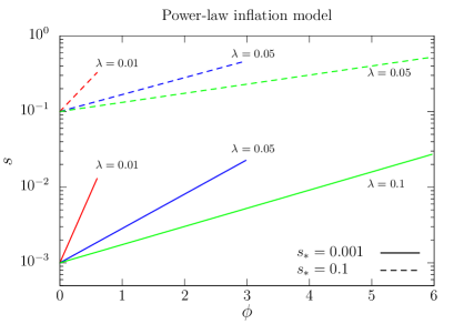

Figure 14 shows the nonlinearity parameter , obtained by using Eq. (3.26), as a function of the spectral index for the power-law inflation model. Similar to Figs. 12, two choices of , 0.001 and 0.1, are considered. The shaded grey region indicates the Planck 2-sigma bound on the spectral index. In the case of with , the nonlinearity parameter may become slightly larger than the Planck 2-sigma bound, . On the other hand, for a relatively large value of such as the case, the nonlinearity parameter tends to be tiny.


Finally, the running of the spectral index , discussed in Appendix A, is presented in Fig. 15. Again, two choices of and three values for the parameter are considered. We observe that, as the spectral index decreases, the running of the spectral index first shows an increasing behaviour, and then it decreases. We further see that the running of the spectral index tends to be smaller when a larger value is considered for . We note that this behaviour aligns with the general analysis presented in Appendix A.
4.3 Hybrid inflation – an example for Class II
The scalar potential for the hybrid inflation model [5] is given by
| (4.7) |
where is the waterfall field, is a mass of , and are dimensionless coupling constants, and is a constant parameter that has the dimension of mass. The inflationary trajectory mainly goes through the valley of the potential along . Thus, during inflation, the hybrid inflation model can effectively be described by a single-field model with the inflaton potential given by
| (4.8) |
where and . The slow-roll parameters (3.14) are given by
| (4.9) |
We are interested in the parameter space where end of inflation is governed by the waterfall phase, not by slow-roll violations. We thus focus on the region so that the slow-roll parameters remain to be smaller than unity for any value of . In this case, the model falls into Class II. We shall view , the field value of the inflaton at the end of inflation, as a free parameter, together with . Once and are fixed, we use 60 -folds, i.e., , to find the field value at the pivot scale and thus the values of the spectral index and the tensor-to-scalar ratio. The original predictions are shown in Fig. 16 for and (magenta lines) by varying . We see that the original model is ruled out by the latest observational constraints.


In Fig. 16, using the analytical expressions (3.22) and (3.25), the spectral index and the tensor-to-scalar ratio in the presence of the assistant field are presented for with for the case of and with for the case of . As expected, the inclusion of the assistant field brings the original predictions to the observationally-favoured region by suppressing the spectral index as well as the tensor-to-scalar ratio. For example, in the case of and , the prediction becomes compatible with the Planck-BK 2-sigma bounds for the range of for and for . In the case of and , the corresponding ranges for the nonminimal coupling parameter are and for and , respectively. Field trajectories for all the parameter choices are shown in Fig. 17.

Figure 18 shows the nonlinearity parameter , obtained by using Eq. (3.26), as a function of the spectral index for the hybrid inflation model. Similar to Fig. 16, two choices of , 0.001 and 0.1, are considered with and . The shaded grey region indicates the Planck 2-sigma bound on the spectral index. In the case of , the nonlinearity parameter may become large. For example, in the cases of , , and , the nonlinearity parameter is incompatible with the Planck 2-sigma bound, . On the other hand, the nonlinearity parameter tends to be tiny in the case.


The running of the spectral index , discussed in Appendix A, is presented in Fig. 19. Similar to Fig. 18, two choices of and two values for are considered. The general tendency of the behaviour of remains the same as those for the previous two example models. In other words, the running of the spectral index shows an increasing behaviour before it decreases again, and it tends to take a smaller value when takes a larger value. For the detailed discussion of the running of the spectral index, see Appendix A.
5 Conclusion
We have investigated the impact of the assistant field on single-field inflationary models. The assistant field is characterised by being nonminimally coupled to gravity, effectively massless, and having no direct coupling to the original inflaton field. Without specifying a potential for the inflaton field, we performed a general analysis and presented analytical expressions for inflationary observables such as the spectral index , the tensor-to-scalar ratio , and the local-type nonlinearity parameter , for both the metric and Palatini formulations.
For Class I, where the end of inflation is achieved through slow-roll violations, the assistant field reduces both and , potentially reviving many single-field models that were previously ruled out by observations. For Class II, where the end of inflation is determined by a separate sector, a small value may bring a small into the observationally-favoured region. The compatibility of the nonlinearity parameter with observations is also shown for both Class I and Class II.
Our results are demonstrated using three example models: loop inflation (Class I), power-law inflation, and hybrid inflation (Class II). These models were previously ruled out due to large values of and/or . Our findings show that the presence of the assistant field can bring the predictions of and into the observationally-favoured region, making the models compatible with the current observational bounds.
It is worth noting that not all single-field models can be revived with the help of the assistant field. For instance, models that originally predict a small and belong to either Class I or Class II with a large cannot be revived. The impact of a massive assistant field on such models remains an open question and will be the subject of future study.
Acknowledgments
This work was supported by National Research Foundation grants funded by the Korean government (NRF-2021R1A4A2001897) and (NRF-2019R1A2C1089334) (S.C.P.), and JSPS KAKENHI Grants No. 19K03874 (T.T.).
Appendix A Running of the Spectral Index
The running of the scalar spectral index in a general multi-field inflation model is given by [70]
| (A.1) |
evaluated at the horizon crossing, which we denote by the subscript , where
| (A.2) |
with being the background fields. For the two-field model under consideration, one finds that
and
where
and
From the definition of in Eq. (A.2), we find that
and
Here, we have defined
Combining all the individual terms, together with Eq. (3.1), into Eq. (A.1) gives the slow-roll-approximated analytical expression for the running of the scalar spectral index. As the calculation is straightforward and the resultant expression is rather long, we do not present the final expression here.


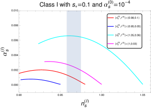


Figure 20 shows the behaviour of the running of the spectral index as a function of the nonminimal coupling parameter (upper panel) and the spectral index (lower panel) for Class I. Two values of , 0.001 (left) and 0.1 (right), are considered, together with various choices of . For all cases, we have fixed to be . We observe that the running of the spectral index first grows as the nonminimal coupling parameter increases. Eventually, the running of the spectral index decreases. This behaviour is similar to that of the nonlinearity parameter. For Class II, the behaviour of the running of the spectral index remains the same as presented in Fig. 21. On top of the various choices for , , and , we have considered two values, and , for .
The latest Planck experiment constrains the running of the spectral index as, e.g., (Planck TT,TE,EE+lowEB+lensing) at 68% C.L. On the other hand, once the running of the running of the spectral index is taken into account, the constraint becomes
| (A.3) |
or (Planck TT,TE,EElowElensing), both at 68% C.L. [1]. For all cases we have considered, . We also note that the running of the spectral index tends to be smaller when takes a larger value, giving , which is well within the allowed bounds obtained with the running of the running, while they are larger than the bounds where the running of the running is not taken into account.
References
- [1] Planck collaboration, Planck 2018 results. X. Constraints on inflation, Astron. Astrophys. 641 (2020) A10 [1807.06211].
- [2] BICEP, Keck collaboration, Improved Constraints on Primordial Gravitational Waves using Planck, WMAP, and BICEP/Keck Observations through the 2018 Observing Season, Phys. Rev. Lett. 127 (2021) 151301 [2110.00483].
- [3] A.D. Linde, Chaotic Inflation, Phys. Lett. B 129 (1983) 177.
- [4] F. Lucchin and S. Matarrese, Power Law Inflation, Phys. Rev. D 32 (1985) 1316.
- [5] M. Cortes and A.R. Liddle, Viable inflationary models ending with a first-order phase transition, Phys. Rev. D 80 (2009) 083524 [0905.0289].
- [6] G.R. Dvali, Q. Shafi and R.K. Schaefer, Large scale structure and supersymmetric inflation without fine tuning, Phys. Rev. Lett. 73 (1994) 1886 [hep-ph/9406319].
- [7] T. Futamase and K.-i. Maeda, Chaotic Inflationary Scenario in Models Having Nonminimal Coupling With Curvature, Phys. Rev. D 39 (1989) 399.
- [8] R. Fakir and W.G. Unruh, Improvement on cosmological chaotic inflation through nonminimal coupling, Phys. Rev. D 41 (1990) 1783.
- [9] J.L. Cervantes-Cota and H. Dehnen, Induced gravity inflation in the standard model of particle physics, Nucl. Phys. B 442 (1995) 391 [astro-ph/9505069].
- [10] E. Komatsu and T. Futamase, Complete constraints on a nonminimally coupled chaotic inflationary scenario from the cosmic microwave background, Phys. Rev. D 59 (1999) 064029 [astro-ph/9901127].
- [11] F.L. Bezrukov and M. Shaposhnikov, The Standard Model Higgs boson as the inflaton, Phys. Lett. B 659 (2008) 703 [0710.3755].
- [12] S.C. Park and S. Yamaguchi, Inflation by non-minimal coupling, JCAP 08 (2008) 009 [0801.1722].
- [13] R.N. Lerner and J. McDonald, Distinguishing Higgs inflation and its variants, Phys. Rev. D 83 (2011) 123522 [1104.2468].
- [14] A. Linde, M. Noorbala and A. Westphal, Observational consequences of chaotic inflation with nonminimal coupling to gravity, JCAP 03 (2011) 013 [1101.2652].
- [15] J. Kim, P. Ko and W.-I. Park, Higgs-portal assisted Higgs inflation with a sizeable tensor-to-scalar ratio, JCAP 02 (2017) 003 [1405.1635].
- [16] L. Boubekeur, E. Giusarma, O. Mena and H. Ramírez, Does Current Data Prefer a Non-minimally Coupled Inflaton?, Phys. Rev. D 91 (2015) 103004 [1502.05193].
- [17] J. Kim and J. McDonald, Chaotic initial conditions for nonminimally coupled inflation via a conformal factor with a zero, Phys. Rev. D 95 (2017) 103501 [1612.04730].
- [18] T. Tenkanen, Resurrecting Quadratic Inflation with a non-minimal coupling to gravity, JCAP 12 (2017) 001 [1710.02758].
- [19] R.Z. Ferreira, A. Notari and G. Simeon, Natural Inflation with a periodic non-minimal coupling, JCAP 11 (2018) 021 [1806.05511].
- [20] I. Antoniadis, A. Karam, A. Lykkas, T. Pappas and K. Tamvakis, Rescuing Quartic and Natural Inflation in the Palatini Formalism, JCAP 03 (2019) 005 [1812.00847].
- [21] T. Takahashi and T. Tenkanen, Towards distinguishing variants of non-minimal inflation, JCAP 04 (2019) 035 [1812.08492].
- [22] M. Shokri, F. Renzi and A. Melchiorri, Cosmic Microwave Background constraints on non-minimal couplings in inflationary models with power law potentials, Phys. Dark Univ. 24 (2019) 100297 [1905.00649].
- [23] T. Takahashi, T. Tenkanen and S. Yokoyama, Violation of slow-roll in nonminimal inflation, Phys. Rev. D 102 (2020) 043524 [2003.10203].
- [24] Y. Reyimuaji and X. Zhang, Natural inflation with a nonminimal coupling to gravity, JCAP 03 (2021) 059 [2012.14248].
- [25] D.Y. Cheong, S.M. Lee and S.C. Park, Reheating in models with non-minimal coupling in metric and Palatini formalisms, JCAP 02 (2022) 029 [2111.00825].
- [26] T. Kodama and T. Takahashi, Relaxing inflation models with nonminimal coupling: A general study, Phys. Rev. D 105 (2022) 063542 [2112.05283].
- [27] A.A. Starobinsky, A New Type of Isotropic Cosmological Models Without Singularity, Phys. Lett. B 91 (1980) 99.
- [28] I.D. Gialamas and A.B. Lahanas, Reheating in Palatini inflationary models, Phys. Rev. D 101 (2020) 084007 [1911.11513].
- [29] I.D. Gialamas, A. Karam and A. Racioppi, Dynamically induced Planck scale and inflation in the Palatini formulation, JCAP 11 (2020) 014 [2006.09124].
- [30] I.D. Gialamas, A. Karam, T.D. Pappas and V.C. Spanos, Scale-invariant quadratic gravity and inflation in the Palatini formalism, Phys. Rev. D 104 (2021) 023521 [2104.04550].
- [31] I.D. Gialamas and K. Tamvakis, Inflation in Metric-Affine Quadratic Gravity, 2212.09896.
- [32] S. Ferrara, R. Kallosh, A. Linde and M. Porrati, Minimal Supergravity Models of Inflation, Phys. Rev. D 88 (2013) 085038 [1307.7696].
- [33] R. Kallosh, A. Linde and D. Roest, Superconformal Inflationary -Attractors, JHEP 11 (2013) 198 [1311.0472].
- [34] S.C. Hyun, J. Kim, S.C. Park and T. Takahashi, Non-minimally assisted chaotic inflation, JCAP 05 (2022) 045 [2203.09201].
- [35] D.I. Kaiser and A.T. Todhunter, Primordial Perturbations from Multifield Inflation with Nonminimal Couplings, Phys. Rev. D 81 (2010) 124037 [1004.3805].
- [36] J. White, M. Minamitsuji and M. Sasaki, Curvature perturbation in multi-field inflation with non-minimal coupling, JCAP 07 (2012) 039 [1205.0656].
- [37] D.I. Kaiser, E.A. Mazenc and E.I. Sfakianakis, Primordial Bispectrum from Multifield Inflation with Nonminimal Couplings, Phys. Rev. D 87 (2013) 064004 [1210.7487].
- [38] R.N. Greenwood, D.I. Kaiser and E.I. Sfakianakis, Multifield Dynamics of Higgs Inflation, Phys. Rev. D 87 (2013) 064021 [1210.8190].
- [39] D.I. Kaiser and E.I. Sfakianakis, Multifield Inflation after Planck: The Case for Nonminimal Couplings, Phys. Rev. Lett. 112 (2014) 011302 [1304.0363].
- [40] J. White, M. Minamitsuji and M. Sasaki, Non-linear curvature perturbation in multi-field inflation models with non-minimal coupling, JCAP 09 (2013) 015 [1306.6186].
- [41] K. Schutz, E.I. Sfakianakis and D.I. Kaiser, Multifield Inflation after Planck: Isocurvature Modes from Nonminimal Couplings, Phys. Rev. D 89 (2014) 064044 [1310.8285].
- [42] S. Kawai and J. Kim, Testing supersymmetric Higgs inflation with non-Gaussianity, Phys. Rev. D 91 (2015) 045021 [1411.5188].
- [43] S. Kawai and J. Kim, Multifield dynamics of supersymmetric Higgs inflation in SU(5) GUT, Phys. Rev. D 93 (2016) 065023 [1512.05861].
- [44] S. Karamitsos and A. Pilaftsis, Frame Covariant Nonminimal Multifield Inflation, Nucl. Phys. B 927 (2018) 219 [1706.07011].
- [45] S. Pi, Y.-l. Zhang, Q.-G. Huang and M. Sasaki, Scalaron from -gravity as a heavy field, JCAP 05 (2018) 042 [1712.09896].
- [46] D.Y. Cheong, S.M. Lee and S.C. Park, Primordial black holes in Higgs- inflation as the whole of dark matter, JCAP 01 (2021) 032 [1912.12032].
- [47] L.-H. Liu and T. Prokopec, Non-minimally coupled curvaton, JCAP 06 (2021) 033 [2005.11069].
- [48] S.M. Lee, T. Modak, K.-y. Oda and T. Takahashi, The -Higgs inflation with two Higgs doublets, Eur. Phys. J. C 82 (2022) 18 [2108.02383].
- [49] D.Y. Cheong, K. Kohri and S.C. Park, The inflaton that could: primordial black holes and second order gravitational waves from tachyonic instability induced in Higgs-R 2 inflation, JCAP 10 (2022) 015 [2205.14813].
- [50] M. Kubota, K.-y. Oda, S. Rusak and T. Takahashi, Double inflation via non-minimally coupled spectator, JCAP 06 (2022) 016 [2202.04869].
- [51] S.R. Geller, W. Qin, E. McDonough and D.I. Kaiser, Primordial black holes from multifield inflation with nonminimal couplings, Phys. Rev. D 106 (2022) 063535 [2205.04471].
- [52] S. Kawai and J. Kim, Primordial black holes and gravitational waves from nonminimally coupled supergravity inflation, 2209.15343.
- [53] K.-Y. Choi, L.M.H. Hall and C. van de Bruck, Spectral Running and Non-Gaussianity from Slow-Roll Inflation in Generalised Two-Field Models, JCAP 02 (2007) 029 [astro-ph/0701247].
- [54] J. Kim, Y. Kim and S.C. Park, Two-field inflation with non-minimal coupling, Class. Quant. Grav. 31 (2014) 135004 [1301.5472].
- [55] A.A. Starobinsky, Multicomponent de Sitter (Inflationary) Stages and the Generation of Perturbations, JETP Lett. 42 (1985) 152.
- [56] D.S. Salopek and J.R. Bond, Nonlinear evolution of long wavelength metric fluctuations in inflationary models, Phys. Rev. D 42 (1990) 3936.
- [57] M. Sasaki and E.D. Stewart, A General analytic formula for the spectral index of the density perturbations produced during inflation, Prog. Theor. Phys. 95 (1996) 71 [astro-ph/9507001].
- [58] M. Sasaki and T. Tanaka, Superhorizon scale dynamics of multiscalar inflation, Prog. Theor. Phys. 99 (1998) 763 [gr-qc/9801017].
- [59] D.H. Lyth, K.A. Malik and M. Sasaki, A General proof of the conservation of the curvature perturbation, JCAP 05 (2005) 004 [astro-ph/0411220].
- [60] Planck collaboration, Planck 2018 results. IX. Constraints on primordial non-Gaussianity, Astron. Astrophys. 641 (2020) A9 [1905.05697].
- [61] S. Camera, M.G. Santos, P.G. Ferreira and L. Ferramacho, Cosmology on Ultra-Large Scales with HI Intensity Mapping: Limits on Primordial non-Gaussianity, Phys. Rev. Lett. 111 (2013) 171302 [1305.6928].
- [62] L.D. Ferramacho, M.G. Santos, M.J. Jarvis and S. Camera, Radio galaxy populations and the multitracer technique: pushing the limits on primordial non-Gaussianity, Mon. Not. Roy. Astron. Soc. 442 (2014) 2511 [1402.2290].
- [63] A. Raccanelli et al., Probing primordial non-Gaussianity via iSW measurements with SKA continuum surveys, JCAP 01 (2015) 042 [1406.0010].
- [64] D. Yamauchi, K. Takahashi and M. Oguri, Constraining primordial non-Gaussianity via a multitracer technique with surveys by Euclid and the Square Kilometre Array, Phys. Rev. D 90 (2014) 083520 [1407.5453].
- [65] S. Camera, M.G. Santos and R. Maartens, Probing primordial non-Gaussianity with SKA galaxy redshift surveys: a fully relativistic analysis, Mon. Not. Roy. Astron. Soc. 448 (2015) 1035 [1409.8286].
- [66] R. de Putter and O. Doré, Designing an Inflation Galaxy Survey: how to measure using scale-dependent galaxy bias, Phys. Rev. D 95 (2017) 123513 [1412.3854].
- [67] J.B. Muñoz, Y. Ali-Haïmoud and M. Kamionkowski, Primordial non-gaussianity from the bispectrum of 21-cm fluctuations in the dark ages, Phys. Rev. D 92 (2015) 083508 [1506.04152].
- [68] D. Yamauchi and K. Takahashi, Probing higher-order primordial non-Gaussianity with galaxy surveys, Phys. Rev. D 93 (2016) 123506 [1509.07585].
- [69] T. Sekiguchi, T. Takahashi, H. Tashiro and S. Yokoyama, Probing primordial non-Gaussianity with 21 cm fluctuations from minihalos, JCAP 02 (2019) 033 [1807.02008].
- [70] J.-O. Gong, Running of scalar spectral index in multi-field inflation, JCAP 05 (2015) 041 [1409.8151].
- [71] K. Kohri, Y. Oyama, T. Sekiguchi and T. Takahashi, Precise Measurements of Primordial Power Spectrum with 21 cm Fluctuations, JCAP 10 (2013) 065 [1303.1688].
- [72] A. Pourtsidou, Synergistic tests of inflation, 1612.05138.
- [73] T. Sekiguchi, T. Takahashi, H. Tashiro and S. Yokoyama, 21 cm Angular Power Spectrum from Minihalos as a Probe of Primordial Spectral Runnings, JCAP 02 (2018) 053 [1705.00405].
- [74] T. Basse, J. Hamann, S. Hannestad and Y.Y.Y. Wong, Getting leverage on inflation with a large photometric redshift survey, JCAP 06 (2015) 042 [1409.3469].
- [75] J.B. Muñoz, E.D. Kovetz, A. Raccanelli, M. Kamionkowski and J. Silk, Towards a measurement of the spectral runnings, JCAP 05 (2017) 032 [1611.05883].
- [76] X. Li, N. Weaverdyck, S. Adhikari, D. Huterer, J. Muir and H.-Y. Wu, The Quest for the Inflationary Spectral Runnings in the Presence of Systematic Errors, Astrophys. J. 862 (2018) 137 [1806.02515].