Nonlocalization of singular potentials in quantum dynamics

As stated in [27, 26], the Gaussian wave packet

is usually adopted as the initial function to test the convergence rate as well as to investigate the quantum tunneling, where $(x^{0},k^{0})$ gives the initial center position and $\sigma$ is the minimum position spread. We will simulate its quantum scattering in the Dirac delta function potential, which has never been reported before in the literature. For the purpose of testing only, we set $\hbar=1~{}\text{eV}\cdot\text{fs}$, $m=1~{}\text{eV}\cdot\text{fs}^{2}\cdot\text{nm}^{-2}$, $x^{0}=-10~{}\text{nm}$, $k^{0}=2~{}\text{nm}^{-1}$, and $\sigma=2~{}\text{nm}$. The computational domain is chosen as $[X_{L},X_{R}]=[-30~{}\text{nm},30~{}\text{nm}]$ which is divided evenly into $Q=20$ cells, $-k_{min}=k_{max}=\pi~{}\text{nm}^{-1}$, and the quantum evolution with a fixed time step $\Delta t=0.01$ fs is stopped at $t_{fin}=10$ fs.

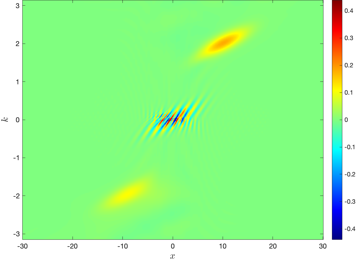
The first test tries $H=1$ in Eq. (1.2) and the resulting Wigner functions at $t=2.5,5,7.5,10$ fs are displayed in Fig. 2, which is obtained on the finest mesh we have tried: $N_{k}=512,M=55$. It is clearly observed there that the wave packet still goes partially through the barrier though the barrier whose height is infinite. That is a clear manifestation of quantum tunneling effect in the Dirac delta function potential [29], reflecting a fundamental difference between quantum world and macroscopic world. A possible explanation is that the width of the Dirac delta function barrier tends to be extremely small, very close to $0$ in particular, albeit the infinitely large height. To study the convergence rate with respect to $N_{k}$, the number of collocation points in each $x$-cell is fixed to be $M=55$. Similarly, when studying the convergence rate with respect to $M$, the number of collocation points in $k$-space is fixed to be $N_{k}=512$. Fig. 3 displays the spectral convergence of $\epsilon_{2}(10)$ and $\epsilon_{\infty}(10)$ against $N_{k}$ or $M$ where we have set $N_{um}=600$ in Eq. (2.7). That is, the numerical results in Fig. 2 are numerically converged.

To be more specific, the uncertainty

is adopted to measure the nonlocality, and its numerical value is still obtained on the uniform mesh given in Eq. (2.7), where $p=\hbar k$ is the momentum. We show in Table 1 that the numerical results with different mesh sizes and find that the numerically converged value for $\sigma_{x}(10)\sigma_{p}(10)$ is $20.8510$ for $H=1$.

In addition to the uncertainty, we continue to use the partial mass

for investigating the tunneling effect for ten different powers: $H=\pm 0.5$, $\pm 1$, $\pm 1.5$, $\pm 2$, and $\pm 2.5$. $P_{r}$ can also be regarded as the tunneling rate in view of that the total mass equals to one. Figs. 4 and 5 show the tunneling rates and uncertainties for potential barriers $H>0$ and potential wells with $H<0$, respectively. The curves in Fig. 4 exhibit the deceleration of $P_{r}(t)$ as $H$ increases, and uncertainty peaking at $H=1$. It can be further found that the moment when the uncertainty reaches the maximum coincides with that the tunneling rate reaches to about $0.5$. At this moment, the variances accumulate the most and it is difficult to observed the position and momentum of the wavepacket simultaneously. Moreover, when the power is high enough, i.e., $H\geq 1.5$, there are significant fluctuations of $\sigma_{x}(t)\,\sigma_{p}(t)$ and $P_{r}(t)$. That could be comprehended as follows. The influence of the power $H$ leads to the high oscillations in the Wigner function at the center $x=0$ nm. Therefore, these two observables fluctuate during the wave packet interacting with the barrier. When it comes to the wells with negative power, it can be observed in Fig. 5 that the trend of the tunneling rate $P_{r}(t)$ is opposite to that of the uncertainty $\sigma_{x}(t)\,\sigma_{p}(t)$: $P_{r}(t)$ decreases and $\sigma_{x}(t)\,\sigma_{p}(t)$ increases as as $|H|$ increases.

The point charge causes singularity because it has no size. In view of this, one may use a finite size model to avoid the singularity. The Gaussian function with size of $a$, denoted by $V_{a}(x)$, is usually used to mimic the point charge model [30, 1], the validity of which relies on the following limit

However, we would like to point out that there is a huge gap between the quantum behavior caused by the point charge $\delta(x)$ and finite-size charge $V_{a}(x)$.

Table 2 displays the numerically converged uncertainties at $t_{fin}=10~{}\text{fs}$ for decreasing sizes. When $a=10^{-16}$ nm, $\sigma_{x}(10)\,\sigma_{p}(10)$ is about $0.8003$, which is far less that $20.8510$ caused by $\delta(x)$. In fact, as the size gradually becomes smaller, the uncertainty first grows to $1.2272$, then gradually decreases, and finally stays around $0.8003$. Such apparent discrepancy can be also observed from the Wigner functions at the final instant in Fig. 6. Compared the Wigner function under $V_{a}(x)$ with $a=0.5$ nm in Fig. 6(a), it is obvious that the Wigner function under $\delta(x)$ in Fig. 6(b) reaches the extrema around $x=0$ nm, where the singular point exactly locates at, and the oscillation between positive and negative values is more vicious. More specifically, at the final instant, the average position and moment are $(\left<\hat{x}\right>_{10},\left<\hat{p}\right>_{10})=(9.7732,1.9840)$ under the Gaussian barrier, but alter to $(\left<\hat{x}\right>_{10},\left<\hat{p}\right>_{10})=(1.1313,0.0047)$ under $\delta(x)$. Fig. 6(c) provides the tunneling rate $P_{r}(t)$. It reaches almost to $1$ as expected under the Gaussian barrier, which is consistent with the weak presence of negative part of the Wigner function in Fig. 6(a). By contrast, it is manifested in Fig. 6(d) that the same wave packet can just partially pass through the Dirac delta function barrier and its uncertainty increases significantly, which should result from the infinite height of the potential.

In a word, our numerical experiments suggests an essential difference between the singular potential and its regularized counterpart as already shown in investigating nuclear magnetic shielding [30]. No matter how small the size of Gaussian barrier we choose, it is still a smooth and local potential. The Dirac delta function potential, on the contrary, an ideal model widely used to simulate the point charge field source of quantum chemical reactions, has some essentially difference from such regularized one in studying quantum phenomena.

In view of the high dimensionality of phase space, the foregoing treatment of singular potentials using the Wigner function approach can be also extended to high-dimensional scenarios. This section is devoted to scattering of the Fermi-Dirac distribution in 4-D phase space under a singular potential. Specifically, we adopt the following position-independent 2-D Fermi-Dirac distribution function [31, 32] as the initial data for the Wigner equation (1.5)

where $m=0.067\,m_{e}$, $m_{e}=5.68562966~{}\text{eV}\cdot\text{fs}^{2}\cdot\text{nm}^{-2}$, $\hbar=0.658211899~{}\text{eV}\cdot\text{fs}$, $k_{B}=8.61734279\times{10}^{-5}~{}\text{eV}\cdot{\text{K}}^{-1}$, $T$ is taken as $300~{}\text{K}$, and $E_{\text{F}}=0.1~{}\text{eV}$ signifies the Fermi energy. Meanwhile, we choose an annular singular potential $V(x_{1},x_{2})=\sum_{i=1}^{8}\delta(x_{1}-d^{i}_{1})\delta(x_{2}-d^{i}_{2})$, where all singular points, numbered $1$ to $8$ in an anti-clockwise direction with the right-most one being the first, are evenly distributed in a circle with radius equal to $2$ nm and $(d_{1}^{i},d_{2}^{i})$ gives the position of the $i$-th singular point.

The computational domain is $\mathcal{X}\times\mathcal{X}\times\mathcal{K}\times\mathcal{K}$ with $\mathcal{X}=[-10~{}\text{nm},10~{}\text{nm}]$ and $\mathcal{K}=[-\pi~{}{\text{nm}}^{-1},\pi~{}{\text{nm}}^{-1}]$. We use the same $N_{k}$ collocation points for all $\mathcal{K}$, the same number of elements $Q=5$ and $M$ collocation points in each element for all $\mathcal{X}$. The quantum dynamics is evolved to $t_{fin}=2.5~{}\text{fs}$ with time step $\Delta t=0.01~{}\text{fs}$. We measure the errors of spatial marginal distribution of the Wigner function,

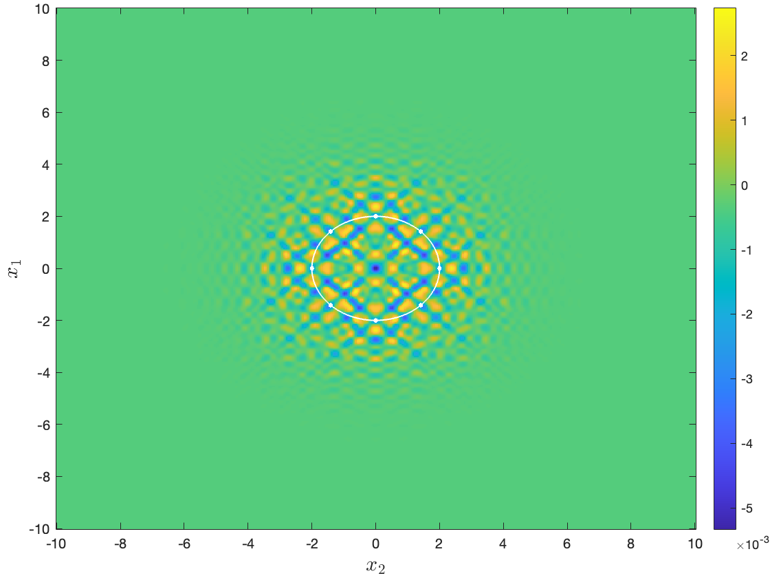
in a similar way to calculating Eqs. (2.5) and (2.6). Fig. 7 presents the errors against $N_{k}$ and $M$ after fixing $N_{um}=400$ in Eq. (2.7) and the spectral convergence is evident again. The spatial marginal distributions on the finest mesh at different instants are displayed in Fig. 8 where the corresponding constant distributions in the free space, $F_{sm}^{free}(x_{1},x_{2},t)\equiv 0.05384$, have been subtracted. It can be observed there that the Fermi-Dirac distribution first reacts strongly to the eight singular points in the circle during which many small oscillations are produced in the central area of the circle, and then gradually expands to the surroundings. Obviously, such expanding is blocked by the eight Dirac delta function potentials and the resulting interference forms $12$ branches outside the circle: $4$ big branches lie in the main directions, north, east, south and west, respectively, and the remaining $8$ small branches are equally distributed between them, where six lines that are determined by pairs of singular points: $(1,7)$, $(2,6)$, $(3,5)$, $(1,3)$, $(4,8)$ and $(5,7)$ serve as the boundaries of branches. Inside the circle, the interference pattern shows a clear square structure that is also shaped by the same six lines. At the final time $t=2.5~{}\text{fs}$, a basin structure emerges: The spatial marginal distribution inside the circle is reduced to less than $F_{sm}^{free}$ (see Fig. 8(i)), and that above $F_{sm}^{free}$ is all outside the circle (see Fig. 8(h)).

Plugging Eq. (3.1) into Eq. (1.7) yields the corresponding Wigner kernel

and then substituting it in Eq. (2.3) leads to

where $\varepsilon$ is a prescribed small parameter and $\tilde{\nu}=2\pi\nu/L_{k}$. Using the the Taylor expansion in $(0,\varepsilon)$ gives

and with the help of the cosine integral function $\operatorname{Ci}(x)=-\int_{x}^{+\infty}\frac{\cos t}{t}\,\mathrm{d}t$,we have

Accordingly, the expansion coefficient $c_{\nu}(x)$ given in an oscillatory improper integral (3.5) can be approximated to the machine resolution by choosing $\varepsilon=1$E-5. Other parameters are set to be: $H=1$, $-X_{L}=X_{R}=30~{}\text{nm}$, $-k_{min}=k_{max}=\pi~{}\text{nm}^{-1}$, $N_{k}=512$, $Q=20$, $M=55$, $\Delta t=0.01~{}\text{fs}$, and $N_{um}=600$. We use an initial Gaussian wave packet close to the origin by setting $x^{0}=-1~{}\text{nm}$ and $k^{0}=0.5~{}\text{nm}^{-1}$ in Eq. (2.8). Numerical convergence tests are given in Fig. 9 and show clearly the spectral accuracy. The left column of Fig. 10 plots the numerically converged Wigner functions at $t=2.5,\,5,\,7.5,\,10$ fs obtained on the finest mesh. It can be observed there that, the wave packet is attracted by the logarithmic potential (3.1), and keeps moving around the singular point, during which many small oscillations appear around the origin along with the singularity.

It has been shown that the Poisson summation formula can be used to approximate the Wigner kernel (1.7) well ($y_{\zeta}=\zeta\,\Delta y$ and $\Delta y$ being the spacing):

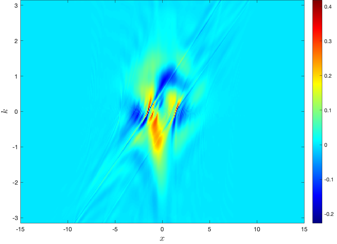
when the external potential $V(x)$ is smooth and localized [26], but fails when taking the Coulomb interaction into account [23]. Here we would like to confirm this failure using the logarithmic potential. After using the “approximate” Wigner kernel (3.6) to replace the analytical one (3.4) and keeping all other settings unchanged, we rerun the simulations in the left column of Fig. 10 and display the resulting Wigner functions in the middle column of Fig. 10, which shows some obvious discrepancy. Compared with the reference solutions, the Wigner functions obtained with Eq. (3.6) display much more severe oscillations with higher peaks and deeper valleys, and the corresponding spatial marginal distributions show some spurious oscillations and non-physical negative values (see the right column of Fig. 10).

According to the Fourier transform of the inverse power function with $\alpha\in(0,1)$: $\mathcal{F}[|x|^{\alpha}](\xi)=-2\sin(\frac{\pi}{2}(\alpha-1))\Gamma(\alpha)|\xi|^{-\alpha}$, the Wigner kernel of Eq. (3.2) reads

where $\Gamma(x)$ gives the Gamma function. Combining Eqs. (3.7) and (2.3) together yields

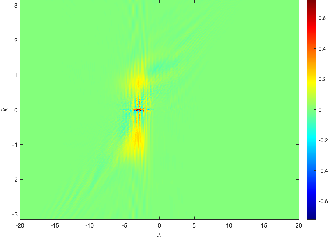
which can be efficiently approximated to the machine accuracy with the help of the Generalized Hypergeometric function ${}_{1}F_{2}((1-\alpha)/2;\,1/2,(3-\alpha)/2;\,x)$ [35]. For example, when $\alpha=1/2$, that Generalized Hypergeometric function reduces to the Fresnel function $\operatorname{C}(x)=\int_{0}^{x}\cos(\pi t^{2}/2)\,\mathrm{d}t$. We adopt the same parameters as in Section 3.1 to simulate the scattering between the Gauss wave packet and the inverse power potential. Fig. 11 shows the spectral convergence with respect to $N_{k}$ and $M$ again, and Fig. 12 the Wigner functions at four different instants. We are able to observe there that the wave packet partially passes through the inverse power potential barrier; and the negative Wigner function, sandwiched between two scattered wave packets in opposite directions, strongly implies the uncertainty principle around the singularity. Fig. 13 further plots the effect of power $\alpha$ on the tunneling rate $P_{r}(t)$ in Eq. (2.10) and uncertainty $\sigma_{x}(t)\,\sigma_{p}(t)$ in Eq. (2.9). It is evident that, the tunneling rate gradually increases as $\alpha$ rises, which reflects that the width of the potential becomes steadily smaller. Since $P_{r}(t)$ never rises over $0.5$ throughout the scattering, the uncertainty $\sigma_{x}(t)\,\sigma_{p}(t)$ shows a mounting tendency whilst $P_{r}(t)$ ascends, which is incurred by the shape change of the potential, namely the increase of $\alpha$.

The Wigner kernel of the inverse square potential (3.3) is

and plugging it into Eq. (2.3), we are able to get a close form for $c_{\nu}(x)$ like Eq. (2.4). The parameters are: $[X_{L},X_{R}]=[-30~{}\text{nm},30~{}\text{nm}]$, $[k_{min},k_{max}]=[-\pi~{}\text{nm}^{-1},\pi~{}\text{nm}^{-1}]$, $N_{k}=512$, $Q=40$, $M=55$, $N_{um}=600$, $\Delta t=0.005~{}\text{fs}$, $H=1$, $x^{0}=-5~{}\text{nm}$, $k^{0}=1~{}\text{nm}^{-1}$. Fig. 14 verifies the spectral convergence against both $N_{k}$ and $M$. Fig. 15 displays the quantum dynamics where the Gaussian wave packet is almost totally reflected after hitting the singular barrier. The tunneling rate $P_{r}(t)$ are $0.01158$, $0.009115$, $0.006731$ and $0.002025$ at $t=2$, $4$, $5$, and $8$ fs, respectively, indicating transparently that it is difficult for the wave packet to pass through the barrier due to the strong singularity of the inverse power potential. This is very different from the scattering shown in Section 3.2 with the inverse power potential which has much weaker singularity. Moreover, severe oscillations of positive and negative Wigner functions clearly appear around the origin, which accords with the summary that the quantum behavior near the singularities is difficult to be measured.

References

- [1] L. Visscher and K. G. Dyall. Dirac–Fock atomic electronic structure calculations using different nuclear charge distributions. Atomic Data and Nuclear Data Tables, 67:207, 1997.
- [2] A. K. Roy. Studies on some singular potentials in quantum mechanics. International Journal of Quantum Chemistry, 104:861, 2005.
- [3] K. M. Case. Singular potentials. Physical Review, 80:797, 1950.
- [4] A. M. Perelomov and V. S. Popov. “Fall to the center” in quantum mechanics. Theoretical and Mathematical Physics, 4:664, 1970.
- [5] K. Meetz. Singular potentials in nonrelativistic quantum mechanics. Il Nuovo Cimento (1955-1965), 34:690, 1964.
- [6] W. M. Frank, D. J. Land, and R. M. Spector. Singular potentials. Reviews of Modern Physics, 43:36, 1971.
- [7] S. Keraani. Wigner measures dynamics in a Coulomb potential. Journal of Mathematical Physics, 46:063512, 2005.
- [8] M. Cinal. Highly accurate numerical solution of Hartree–Fock equation with pseudospectral method for closed-shell atoms. Journal of Mathematical Chemistry, 58:1571, 2020.
- [9] G. W. Wei. Discrete singular convolution for the solution of the Fokker–Planck equation. Journal of Chemical Physics, 110:8930, 1999.
- [10] G. Esposito. Scattering from singular potentials in quantum mechanics. Journal of Physics A: Mathematical and General, 31:9493, 1998.
- [11] S. Tan. Energetics of a strongly correlated Fermi gas. Annals of Physics, 323:2952, 2008.
- [12] M. F. Gusson, A. O. O. Gonçalves, R. O. Francisco, R. G. Furtado, J. C. Fabris, and J. A. Nogueira. Dirac -function potential in quasiposition representation of a minimal-length scenario. European Physical Journal C, 78:1, 2018.
- [13] M. W. Ray, E. Ruokokoski, S. Kandel, M. Möttönen, and D. S. Hall. Observation of Dirac monopoles in a synthetic magnetic field. Nature, 505:657, 2014.
- [14] C. G. Gal, A. Giorgini, and M. Grasselli. The nonlocal Cahn–Hilliard equation with singular potential: well-posedness, regularity and strict separation property. Journal of Differential Equations, 263:5253, 2017.
- [15] M. Belloni and R. W. Robinett. The infinite well and Dirac delta function potentials as pedagogical, mathematical and physical models in quantum mechanics. Physics Reports, 540:25, 2014.
- [16] R. Araya, E. Behrens, and R. Rodríguez. A posteriori error estimates for elliptic problems with Dirac delta source terms. Numerische Mathematik, 105:193, 2006.
- [17] R. Scott. Finite element convergence for singular data. Numerische Mathematik, 21:317, 1973.
- [18] E. Wigner. On the quantum correction for thermodynamic equilibrium. Physical Review, 40:749, 1932.
- [19] T. L. Curtright, D. B. Fairlie, and C. K. Zachos. A concise treatise on quantum mechanics in phase space. World Scientific Publishing Company, 2013.
- [20] M. D’Elia, Q. Du, C. Glusa, M. Gunzburger, X. Tian, and Z. Zhou. Numerical methods for nonlocal and fractional models. Acta Numerica, 29:1124, 2020.
- [21] L. Greengard, S. Jiang, and Y. Zhang. The anisotropic truncated kernel method for convolution with free-space Green’s functions. SIAM Journal on Scientific Computing, 40:A3733, 2018.
- [22] F. Vico, L. Greengard, and M. Ferrando. Fast convolution with free-space Green’s functions. Journal of Computational Physics, 323:191, 2016.
- [23] Y. Xiong, Y. Zhang, and S. Shao. A characteristic-spectral-mixed scheme for six-dimensional Wigner-Coulomb dynamics. arXiv:2205.02380, 2022.
- [24] B. Li and J. Shen. The Wigner(–Poisson)–Fokker–Planck equation with singular potential. Applicable Analysis, 96:563, 2017.
- [25] Ilišević, D. and Turnšek, A. Stability of the Wigner equation–a singular case. Journal of Mathematical Analysis and Applications, 429:273, 2015.
- [26] Y. Xiong, Z. Chen, and S. Shao. An advective-spectral-mixed method for time-dependent many-body Wigner simulations SIAM Journal on Scientific Computing, 38:B491, 2016.
- [27] S. Shao, T. Lu, and W. Cai. Adaptive conservative cell average spectral element methods for transient Wigner equation in quantum transport. Communications in Computational Physics, 9:711, 2011.
- [28] Z. Chen, S. Shao, and W. Cai. A high order efficient numerical method for 4-D Wigner equation of quantum double-slit interferences. Journal of Computational Physics, 396, 2019.
- [29] H. Grabert and U. Weiss. Quantum tunneling rates for asymmetric double-well systems with Ohmic dissipation. Physical Review Letters, 54:1605, 1985.
- [30] Y. Xiao, W. Liu, L. Cheng, and D. Peng. Four-component relativistic theory for nuclear magnetic shielding constants: Critical assessments of different approaches. Journal of Chemical Physics, 126:214101, 2007.
- [31] Z. Chen, H. Jiang, and S. Shao. A higher-order accurate operator splitting spectral method for the Wigner–Poisson system. Journal of Computational Electronics, 21:756, 2022.
- [32] A. J. MacLeod. Algorithm 779: Fermi-Dirac functions of order-1/2, 1/2, 3/2, 5/2. ACM Transactions on Mathematical Software (TOMS), 24:1-12, 1998.
- [33] R. Serber. Scaling law for high-energy elastic scattering. Physical Review Letters, 13:32, 1964.
- [34] G. Tiktopoulos. High-energy large-angle scattering by singular potentials. Physical Review., 138:B1550, 1965.
- [35] E. T. Whittaker and G. N. Watson. A course of modern analysis: an introduction to the general theory of infinite processes and of analytic functions; with an account of the principal transcendental functions. University Press, 1915.
- [36] M. Xia, S. Shao, and T. Chou. A frequency-dependent p-adaptive technique for spectral methods. Journal of Computational Physics, 446:110627, 2021.
- [37] M. Xia, S. Shao, and T. Chou. Efficient scaling and moving techniques for spectral methods in unbounded domains. SIAM Journal on Scientific Computing, 43:A3244-A3268, 2021.
- [38] T. Chou, S. Shao, and M. Xia. Adaptive Hermite spectral methods in unbounded domains. Applied Numerical Mathematics, 183:201-220, 2023.