Nonlocal Attention Operator: Materializing Hidden Knowledge Towards Interpretable Physics Discovery
Abstract
Despite the recent popularity of attention-based neural architectures in core AI fields like natural language processing (NLP) and computer vision (CV), their potential in modeling complex physical systems remains under-explored. Learning problems in physical systems are often characterized as discovering operators that map between function spaces based on a few instances of function pairs. This task frequently presents a severely ill-posed PDE inverse problem. In this work, we propose a novel neural operator architecture based on the attention mechanism, which we coin Nonlocal Attention Operator (NAO), and explore its capability towards developing a foundation physical model. In particular, we show that the attention mechanism is equivalent to a double integral operator that enables nonlocal interactions among spatial tokens, with a data-dependent kernel characterizing the inverse mapping from data to the hidden parameter field of the underlying operator. As such, the attention mechanism extracts global prior information from training data generated by multiple systems, and suggests the exploratory space in the form of a nonlinear kernel map. Consequently, NAO can address ill-posedness and rank deficiency in inverse PDE problems by encoding regularization and achieving generalizability. We empirically demonstrate the advantages of NAO over baseline neural models in terms of generalizability to unseen data resolutions and system states. Our work not only suggests a novel neural operator architecture for learning interpretable foundation models of physical systems, but also offers a new perspective towards understanding the attention mechanism.
1 Introduction
The interpretability of machine learning (ML) models has become increasingly important from the security and robustness standpoints (Rudin et al., 2022; Molnar, 2020). This is particularly true in physics modeling problems that can affect human lives, where not only the accuracy but also the transparency of data-driven models are essential in making decisions (Coorey et al., 2022; Ferrari and Willcox, 2024). Nevertheless, it remains challenging to discover the underlying physical system and the governing mechanism from data. Taking the material modeling task for instance, given that only the deformation field is observable, the goal of discovering the underlying material parameter field and mechanism presents an ill-posed unsupervised learning task. That means, even if an ML model can serve as a good surrogate to predict the corresponding loading field from a given deformation field, its inference of the material parameters can still drastically deteriorate.

To discover an interpretable mechanism for physical systems, a major challenge is to infer the governing laws of these systems that are often high- or infinite-dimensional, from data that are comprised of discrete measurements of continuous functions. Therefore, a data-driven surrogate model needs to learn not only the mapping between input and output function pairs, but also the mapping from given function pairs to the hidden state. From the PDE-based modeling standpoint, learning a surrogate model corresponds to a forward problem, whereas inferring the underlying mechanism is an inverse problem. The latter is generally an enduring ill-posed problem, especially when the measurements are scarce. Unfortunately, such an ill-posedness issue may become even more severe in neural network models, due to the inherent bias of neural network approximations (Xu et al., 2019). To tackle this challenge, many deep learning methods have recently been proposed as inverse PDE solvers (Fan and Ying, 2023; Molinaro et al., 2023; Jiang et al., 2022; Chen et al., 2023). The central idea is to incorporate prior information into the learning scheme, in the form of governing PDEs (Yang et al., 2021; Li et al., 2021), regularizers (Dittmer et al., 2020; Obmann et al., 2020; Ding et al., 2022; Chen et al., 2023), or additional operator structures (Uhlmann, 2009; Lai et al., 2019; Yilmaz, 2001). However, such prior information is often either unavailable or problem-specific in complex systems. As a result, these methods can only solve the inverse problem for a particular system, and one has to start from scratch when the system varies (e.g., when the material of the specimen undergoes degradation in a material modeling task).
In this work, we propose Nonlocal Attention Operator (NAO), a novel attention-based neural operator architecture to simultaneously solve both forward and inverse modeling problems. Neural operators (NOs) (Li et al., 2020a, c) learn mappings between infinite-dimensional function spaces in the form of integral operators, hence they provide promising tools for the discovery of continuum physical laws by manifesting the mapping between spatial and/or spatiotemporal data; see You et al. (2022); Liu et al. (2024a, b, 2023); Ong et al. (2022); Cao (2021); Lu et al. (2019, 2021); Goswami et al. (2022); Gupta et al. (2021) and references therein. However, most NOs focus on providing an efficient surrogate for the underlying physical system as a forward solver. They are often employed as black-box universal approximators but lack interpretability of the underlying physical laws. In contrast, the key innovation of NAO is that it introduces a kernel map based on the attention mechanism for simultaneous learning of the operator and the kernel map. As such, the kernel map automatically infers the context of the underlying physical system in an unsupervised manner. Intuitively, the attention mechanism extracts hidden knowledge from multiple systems by providing a function space of identifiability for the kernels, which acts as an automatic data-driven regularizer and endows the learned model’s generalizability to new and unseen system states.
In this context, NAO learns a kernel map using the attention mechanism and simultaneously solves both the forward and inverse problems. The kernel map, whose parameters extract the global information about the kernel from multiple systems, efficiently infers resolution-invariant kernels from new datasets. As a consequence, NAO can achieve interpretability of the nonlocal operator and enable the discovery of hidden physical laws. Our key contributions include:
-
•
We bridge the divide between inverse PDE modeling and physics discovery tasks, and present a method to simultaneously perform physics modeling (forward PDE) and mechanism discovery (inverse PDE).
-
•
We propose a novel neural operator architecture NAO, based on the principle of contextual discovery from input/output function pairs through a kernel map constructed from multiple physical systems. As such, NAO is generalizable to new and unseen physical systems, and offers meaningful physical interpretation through the discovered kernel.
-
•
We provide theoretical analysis to show that the attention mechanism in NAO acts to provide the space of identifiability for the kernels from the training data, which reveals its ability to resolve ill-posed inverse PDE problems.
-
•
We conduct experiments on zero-shot learning to new and unseen physical systems, demonstrating the generalizability of NAO in both forward and inverse PDE problems.
2 Background and related work
Our work resides at the intersection of operator learning, attention-based models, and forward and inverse problems of PDEs. The ultimate goal is to model multiple physical systems from data while simultaneously discovering the hidden mechanism.
Neural operator for hidden physics. Learning complex physical systems directly from data is ubiquitous in scientific and engineering applications (Ghaboussi et al., 1998; Liu et al., 2024c; Ghaboussi et al., 1991; Carleo et al., 2019; Karniadakis et al., 2021; Zhang et al., 2018; Cai et al., 2022; Pfau et al., 2020; He et al., 2021; Besnard et al., 2006). In many applications, the underlying governing laws are unknown, hidden in data to be revealed by physical models. Ideally, these models should be interpretable for domain experts, who can then use these models to make further predictions and expand the understanding of the target physical system. Also, these models should be resolution-invariant. Neural operators are designed to learn mappings between infinite-dimensional function spaces (Li et al., 2020a, b, c; You et al., 2022; Ong et al., 2022; Cao, 2021; Lu et al., 2019, 2021; Goswami et al., 2022; Gupta et al., 2021). As a result, NOs provide a promising tool for the discovery of continuum physical laws by manifesting the mapping between spatial and/or spatio-temporal data.
Forward and inverse PDE problems. Most current NOs focus on providing an efficient surrogate for the underlying physical system as a forward PDE solver. They are often employed as black-box universal approximators without interpretability of the underlying physical laws. Conversely, several deep learning methods have been proposed as inverse PDE solvers (Fan and Ying, 2023; Molinaro et al., 2023; Jiang et al., 2022; Chen et al., 2023), aiming to reconstruct the parameters in the PDE from solution data. Compared to the forward problem, the inverse problem is typically more challenging due to its ill-posed nature. To tackle the ill-posedness, many NOs incorporate prior information, in the form of governing PDEs (Yang et al., 2021; Li et al., 2021), regularizers (Dittmer et al., 2020; Obmann et al., 2020; Ding et al., 2022; Chen et al., 2023), or additional operator structures (Uhlmann, 2009; Lai et al., 2019; Yilmaz, 2001). To our knowledge, our NO architecture is the first that solves both the forward (physics prediction) and inverse (physics discovery) problems simultaneously.
Attention mechanism. Since 2017, the attention mechanism has become the backbone of state-of-the-art deep learning models on many core AI tasks like NLP and CV. By calculating the similarity among tokens, the attention mechanism captures long-range dependencies between tokens (Vaswani et al., 2017). Then, the tokens are spatially mixed to obtain the layer output. Based on the choice of mixers, attention-based models can be divided into three main categories: discrete graph-based attentions (Child et al., 2019; Ho et al., 2019; Wang et al., 2020; Katharopoulos et al., 2020), MLP-based attentions (Tolstikhin et al., 2021; Touvron et al., 2022; Liu et al., 2021), and convolution-based attentions (Lee-Thorp et al., 2021; Rao et al., 2021; Guibas et al., 2021; Nekoozadeh et al., 2023). While most attention models focus on discrete mixers, it is proposed in Guibas et al. (2021); Nekoozadeh et al. (2023); Tsai et al. (2019); Cao (2021); Wei and Zhang (2023) to frame token mixing as a kernel integration, with the goal of obtaining predictions independent of the input resolution.
Along the line of PDE-solving tasks, various attention mechanisms have been used to enlarge model capacity. To improve the accuracy of forward PDE solvers, Cao (2021) removes the softmax normalization in the attention mechanism and employs linear attention as a learnable kernel in NOs. Further developments include the Galerkin-type linear attention in an encoder-decoder architecture in OFormer (Li et al., 2022), a hierarchical transformer for learning multiscale problems (Liu et al., 2022), and a heterogeneous normalized attention with a geometric gating mechanism (Hao et al., 2023) to handle multiple input features. In particular, going beyond solving a single PDE, the foundation model feature of attention mechanisms has been applied towards solving multiple types of PDEs within a specified context in Yang and Osher (2024); Ye et al. (2024); Sun et al. (2024); Zhang (2024). However, to our best knowledge, none of the existing work discovers hidden physics from data, nor do they discuss the connections between the attention mechanism and the inverse PDE problem.
3 Nonlocal Attention Operator
Consider multiple physical systems that are described by a class of operators mapping from input functions to output functions . Our goal is to learn the common physical law, in the form of operators with system-dependent kernels :
| (1) |
Here and are Banach spaces, denotes an additive noise describing the discrepancy between the ground-truth operator and the optimal surrogate operator, and is a kernel function representing the nonlocal spatial interaction. As such, the kernel provides the knowledge of its corresponding system, while (1) offers a zero-shot prediction model for new and unseen systems.
To formulate the learning, we consider training datasets from different systems, with each dataset containing function pairs :
| (2) |
In practice, the data of the input and output functions are on a spatial mesh . The models with kernels correspond to different material micro-structures or different parametric settings. As a demonstration, we consider models for heterogeneous materials with operators in the form
| (3) |
where is a functional of determined by the operator; for example in Section 5.3. Our approach extends naturally to other forms of operators, such as those with radial interaction kernels in Section 5.1 and heterogeneous interaction in the form of . Additionally, for simplicity, we consider scalar-valued functions and and note that the extension to vector-valued functions is trivial.
Remark: Such an operator learning problem arises in many applications in forward and inverse PDE-solving problems. The inference of the kernel is an inverse problem, and the learning of the nonlocal operator is a forward problem. When considering a single physical system and taking in (3) as an input-independent kernel, classical NOs can be obtained for forward PDE-solving tasks (Li et al., 2020c; Guibas et al., 2021) and governing law learning tasks (You et al., 2021; Jafarzadeh et al., 2024). Different from existing work, we consider the operator learning across multiple systems.
3.1 Kernel map with attention mechanism
The key ingredient in NAO is a kernel map constructed using the attention mechanism. It maps from data pairs to an estimation of the underlying kernel. The kernel map
| (4) |
has parameters estimated from the training dataset (2). As such, it maps from the token of the dataset to a kernel estimator, acting as an inverse PDE solver.
A major innovation of this kernel map is its dependence on both and through their tokens. Thus, our approach distinguishes itself from the forward problem-solving NOs in the related work section, where the attention depends only on .
We first transfer the data to tokens according to the operator in (3) by
| (5) | ||||
where and , assuming that has a spatial mesh .
Then, our discrete -layer attention model for the inverse PDE problem writes:
| (6) |
Here, and the attention function is
The kernel map is defined as
| (7) | ||||
where are learnable parameters. Here, we note that only controls the rank bound when lifting each point-wise feature via . In the following, we denote , which characterizes the (trainable) interaction of input function pair instances.
3.2 Nonlocal Attention Operator in continuum limit
As suggested by Cao (2021), we take the activation function as a linear operator. Then, noting that the matrix multiplication in (6) is a Riemann sum approximation of an integral (with a full derivation in Appendix A), we propose the nonlocal attention operator as the continuum limit of (6):
| (14) | |||
| (15) |
in which the integration is approximated by the Riemann sum in our implementation. Here,
We learn the parameters by minimizing the following mean squared error loss function:
| (16) |
The performance of the model is evaluated on test tasks with new and unseen kernels based on the following two criteria:
| Operator (forward PDE) Error: | (17) | |||
| Kernel (inverse PDE) Error: | (18) |
Here, is the empirical measure in the kernel space as defined in Lu et al. (2023). Note that are trained using multiple datasets. Intuitively speaking, the attention mechanism helps encode the prior information from other tasks for learning the nonlocal kernel, and leads to estimators significantly better than those using a single dataset. To formally understand this mechanism, we analyze a shallow 2-layer NAO in the next section.
4 Understanding the attention mechanism
To facilitate further understanding of the attention mechanism, we analyze the limit of the two-layer attention-parameterized kernel in (7) and the range of the kernel map, which falls in the space of identifiability for the kernels from the training data. We also connect the kernel map with the regularized estimators. For simplicity, we consider operators of the form
| (19) |
which is the radial nonlocal kernel in Sec.5.1.
4.1 Limit of the two-layer attention-parameterized kernel
We show that as the number and the spatial mesh approach infinity, the limit of the two-layer attention-parameterized kernel is a double integral. Its proof is in Appendix B.1.
For simplicity, we assume that the dataset in (2) has and with a uniform mesh . We define the tokens by
| (20) |
where and is the spatial mesh for ’s independent variable .
Lemma 4.1.
4.2 Space of identifiability for the kernels
For a given training dataset, we show that the function space in which the kernels can be identified is the closure of a data-adaptive reproducing kernel Hilbert space (RKHS). This space contains the range of the kernel map and hence provides the ground for analyzing the inverse problem.
Lemma 4.2 (Space of Identifiability).
Assume that the training data pairs in (2) are sampled from continuous functions with a compact support. Then, the function space the loss function in (16) has a unique minimizer is the closure of a data-adaptive RKHS with a reproducing kernel determined by the training data:
where is the density of the empirical measure defined by
| (22) |
and the function is defined by
The above space is data-adaptive since the integral kernel depends on data. It characterizes the information in the training data for estimating the nonlocal kernel . In general, the more data, the larger the space is. On the other hand, note that the loss function’s minimizer with respect to is not the kernel map. The minimizer is a fixed estimator for the training dataset and does not provide any information for estimating the kernel from another dataset.
Comparison with regularized estimators. The kernel map solves the ill-posed inverse problem using prior information from the training dataset of multiple systems, which is not used in classical inverse problem solvers. To illustrate this mechanism, consider the extreme case of estimating the kernel in the nonlocal operator from a dataset consisting of only a single function pair . This inverse problem is severely ill-posed because of the small dataset and the need for deconvolution to estimate the kernel. Thus, regularization is necessary, where two main challenges present: (i) the selection of a proper regularization with limited prior information, and (ii) the prohibitive computational cost of solving the resulting large linear systems many times.
In contrast, our kernel map , with the parameter estimated from the training datasets, acts on the token of to provide an estimator. It passes the prior information about the kernel from the training dataset to the estimation for new datasets. Importantly, it captures the nonlinear dependence of the estimator on the data . Computationally, it can be applied directly to multiple new datasets without solving the linear systems. In Section B.2, we further show that a regularized estimator depends nonlinearly on the data pair . In particular, similar to Lemma 4.1, there is an RKHS determined by the data pair . The regularized estimator suggests that the kernel map can involve a component quadratic in the feature , similar to the limit form of the attention model in Lemma 4.1.
5 Experiments
We assess the performance of NAO on a wide range of physics modeling and discovery datasets. Our evaluation focuses on several key aspects: 1) we demonstrate the merits of the continuous and linear attention mechanism, compare the performance with the baseline discrete attention model (denoted as Discrete-NAO), the softmax attention mechanism (denoted as Softmax-NAO), with input on only (denoted as NAO-u), the convolution-based attention mechanism (denoted as AFNO (Guibas et al., 2021)), and an MLP-based encoder architecture that maps the datum directly to a latent kernel (denoted as Autoencoder); 2) we measure the generalizability, in particular, the zero-shot prediction performance in modeling a new physical system with unseen governing equations, and across different resolutions; 3) we evaluate the data efficiency-accuracy trade-off in ill-posed inverse PDE learning tasks, as well as the interpretability of the learned kernels. In all experiments, the optimization is performed with the Adam optimizer. To conduct fair comparison for each method, we tune the hyperparameters, including the learning rates, the decay rates, and the regularization parameters, to minimize the training loss. In all examples, we use 3-layer models, and parameterize the kernel network and with a 3-layer MLP with hidden dimensions and LeakyReLU activation. Experiments are conducted on a single NVIDIA GeForce RTX 3090 GPU with 24 GB memory. Additional details on data generation and training strategies are provided in Appendix C.
5.1 Radial kernel learning
| Case | model | #param | Operator test error | Kernel test error | ||
|---|---|---|---|---|---|---|
| ID | OOD1 | ID | OOD1 | |||
| Discrete-NAO | 16526 | 1.33% | 25.81% | 29.02% | 28.80% | |
| Softmax-NAO | 18843 | 13.45% | 66.06% | 67.55% | 85.80% | |
| = 302, =10 | AFNO | 19605 | 22.62% | 68.76% | - | - |
| NAO | 18843 | 1.48% | 8.10% | 5.40% | 10.02% | |
| NAO-u | 18842 | 13.68% | 66.68% | 20.46% | 74.03% | |
| Autoencoder | 16424 | 12.97% | 1041.49% | 22.56% | 136.79% | |
| = 302, =5 | Discrete-NAO | 10465 | 1.63% | 15.80% | 33.21% | 30.39% |
| NAO | 12783 | 2.34% | 9.23% | 6.87% | 14.62% | |
| = 302, =20 | Discrete-NAO | 28645 | 1.35% | 18.70% | 35.49% | 30.81% |
| NAO | 30963 | 1.33% | 9.12% | 4.63% | 9.14% | |
| = 100, =10 | Discrete-NAO | 8446 | 1.73% | 14.92% | 34.52% | 35.20% |
| NAO | 10763 | 1.07% | 6.35% | 7.41% | 17.02% | |
| = 50, =10 | Discrete-NAO | 6446 | 2.29% | 10.31% | 41.80% | 45.30% |
| NAO | 8763 | 1.56% | 7.19% | 15.95% | 29.47% | |
| = 30, =10 | Discrete-NAO | 5646 | 5.60% | 11.31% | 58.24% | 64.23% |
| NAO | 7963 | 2.94% | 8.04% | 22.65% | 33.77% | |
In this example, we consider the learning of nonlocal diffusion operators, in the form:
| (23) |
Unlike a (local) differential operator, this operator depends on the function nonlocally through the convolution of , and the operator is characterized by a radial kernel . It finds broad physical applications in describing fracture mechanics (Silling, 2000), anomalous diffusion behaviors (Bucur et al., 2016), and the homogenization of multiscale systems (Du et al., 2020).
In this context, our goal is to learn the operator as well as to discover the hidden mechanism, namely the kernel . In the form of the operator in (19), we have and for .
To generate the training data, we consider sine-type kernels
| (24) |
Here, denotes task index. We generate data pairs with a fixed resolution for each task, where the loading function is computed by the adaptive Gauss-Kronrod quadrature method. Then, we form a training sample of each task by taking pairs from this task. When taking the token size , each task contains samples. We consider two test kernels: one following the same rule of (24) with (denoted as the “in-distribution (ID) test” system), and the other following a different rule (denoted as the “out-of-distribution (OOD) test1” system):
| (25) |
Both the operator error (17) and the kernel error (18) are provided in Table 1. While the former measures the error of the learned forward PDE solver (i.e., learning a physical model), the latter demonstrates the capability of serving as an inverse PDE solver (i.e., physics discovery).
Ablation study. We first perform an ablation study on NAO, by comparing its performance with its variants (Discrete-NAO, Softmax-NAO, and NAO-u), AFNO, and Autoencoder, with a fixed token dimension , query-key feature size , and data resolution . When comparing the operator errors, both Discrete-NAO and NAO serve as good surrogate models for the ID task with relative errors of and , respectively, while the other three baselines show errors. Therefore, we focus more on the comparison between Discrete-NAO and NAO. This gap becomes more pronounced in the OOD task: only NAO is able to provide a surrogate of with error, who outperforms its discrete mixer counterpart by , indicating that NAO learns a more generalizable mechanism. This argument is further affirmed when comparing the kernel errors, where NAO substantially outperforms all baselines by at least in the ID test and in the OOD test. This study verifies our analysis in Section 4: NAO learns the kernel map in the space of identifiability, and hence possesses advantages in solving the challenging ill-posed inverse problem. Additionally, we vary the query-key feature size from to and . Note that determines the rank bound of , the matrix that characterizes the interaction between different data pairs. Discrete-NAO again performs well only in approximating the operator for the ID test, while NAO achieves consistent results in both tests and criteria, showing that it has successfully discovered the intrinsic low-dimension in the kernel space.


Alleviating ill-posedness. To further understand NAO’s capability as an inverse PDE solver, we reduce the number of data pairs for each sample from to , making it more ill-posed as an inverse PDE problem. NAO again outperforms its discrete mixer counterpart in all aspects. Interestingly, the errors in NAO increase almost monotonically, showing its robustness. For Discrete-NAO, the error also increases monotonically in the ID operator test, but there exists no consistent pattern in other test criteria. Figure 2 shows the learned test kernels in both the ID and OOD tasks. It shows that Discrete-NAO learns highly oscillatory kernels, while our continuous NAO only has a discrepancy near . Note that when , we have in the ground-truth operator (23), and hence the kernel value at this point does not change the operator value. That means, our data provides almost no information at this point. This again verifies our analysis: continuous NAO learns the kernel map structure from small data based on prior knowledge from other task datasets.
Cross-resolution. We test the NAO model trained with on a dataset corresponding to , and plot the results in Figure 2 Left. The predicted kernel is very similar to the one learned from the same resolution, and the error is also on-par ( versus ).
| model | #param | Operator test error | Kernel test error | |||||
|---|---|---|---|---|---|---|---|---|
| ID | OOD1 | OOD2 | ID | OOD1 | OOD2 | |||
| sine only: Train on sine dataset, 105 samples in total | ||||||||
| 10 | Discrete-NAO | 16526 | 1.33% | 25.81% | 138.00% | 29.02% | 28.80% | 97.14% |
| NAO | 18843 | 1.48% | 8.10% | 221.04% | 5.40% | 10.02% | 420.60% | |
| 20 | Discrete-NAO | 28645 | 1.35% | 18.70% | 99.50% | 35.49% | 30.81% | 101.08% |
| NAO | 30963 | 1.33% | 9.12% | 211.78% | 4.63% | 9.14% | 329.66% | |
| 40 | Discrete-NAO | 52886 | 1.30% | 31.37% | 49.83% | 38.89% | 30.02% | 129.84% |
| NAO | 55203 | 0.67% | 7.34% | 234.43% | 4.03% | 12.16% | 1062.3% | |
| Autoencoder | 16424 | 12.97% | 1041.49% | 698.72% | 22.56% | 136.79% | 304.37% | |
| sine+cosine+polyn: Train on diverse (sine, cosine and polynomial) dataset, 315 samples in total | ||||||||
| 10 | Discrete-NAO | 16526 | 2.27% | 13.02% | 11.50% | 10.41% | 30.79% | 77.80% |
| NAO | 18843 | 2.34% | 14.37% | 10.05% | 7.26% | 28.23% | 94.38% | |
| 20 | Discrete-NAO | 28645 | 1.60% | 6.03% | 19.73% | 21.83% | 21.29% | 18.97% |
| NAO | 30963 | 1.64% | 3.25% | 3.58% | 5.45% | 8.87% | 15.82% | |
| 40 | Discrete-NAO | 52886 | 1.45% | 5.49% | 18.26% | 20.07% | 19.46% | 18.44% |
| NAO | 55203 | 1.54% | 3.09% | 7.69% | 5.04% | 6.92% | 10.48% | |
| Autoencoder | 56486 | 12.67% | 341.96% | 211.61% | 27.06% | 52.43% | 128.08% | |
| Single task: Train on a single sine dataset, 105 samples in total | ||||||||
| 10 | NAO | 18843 | 104.49% | 104.37% | 56.64% | 100.31% | 100.00% | 94.98% |
| 20 | NAO | 30963 | 116.89% | 105.52% | 85.40% | 99.02% | 99.55% | 98.37% |
| 40 | NAO | 55203 | 111.33% | 104.12% | 76.78% | 101.61% | 100.33% | 95.90% |
| Fewer samples: Train on diverse (sine, cosine and polynomial) dataset, 105 samples in total | ||||||||
| 10 | NAO | 18843 | 4.23% | 15.34% | 11.13% | 10.11% | 25.23% | 97.63% |
| 20 | NAO | 30963 | 4.15% | 10.15% | 9.59% | 8.84% | 23.08% | 20.05% |
| 40 | NAO | 55203 | 3.69% | 11.67% | 6.08% | 9.19% | 24.04% | 25.58% |
More diverse tasks. To further evaluate the generalization capability of NAO as a foundation model, we add another two types of kernels into the training dataset. The training dataset is now constructed based on 21 kernels of three groups, with samples on each kernel:
-
•
sine-type kernels: , .
-
•
cosine-type kernels: , .
-
•
polynomial-type kernels: , , where is the degree- Legendre polynomial.


Based on this enriched dataset, besides the original “sine only” setting, three additional settings are considered to compare the generalizability across different settings. The results are reported in Table 2 and Figure 3. In addition to the original setting corresponding to all “sine” kernels, in part II of Table 2 (denoted as “sine+cosine+polyn”), we consider a “diverse task” setting, where all samples are employed in training. In part III, we consider a “single task” setting, where only the first sine-type kernel, , is considered as the training task, with samples on this task. Lastly, in part IV we demonstrate a “fewer samples” setting, where the training dataset still consists of all tasks but with only samples on each task. For testing, besides the ID and OOD tasks in the ablation study, we add an additional OOD task with a Gaussian-type kernel , which is substantially different from all training tasks.
As shown in Table 2, considering diverse datasets helps in both OOD tests (the kernel error is reduced from to in OOD test 1, and from to in OOD test 2), but not for the ID test (the kernel error is slightly increased from to ). We also note that since the “sine only” setting only sees systems with the same kernel frequency in training, it does not generalize to OOD test 2, where it becomes necessary to include more diverse training tasks. As the training tasks become more diverse, the intrinsic dimension of kernel space increases, requiring a larger rank size of the weight matrices. When comparing the “fewer samples” setting with the “sine only” setting, the former exhibits better task diversity but fewer samples per task. One can see that the performance deteriorates on the ID test but improves on OOD test 2. This observation emphasizes the balance between the diversity of tasks and the number of training samples per task.
5.2 Solution operator learning
We consider the modeling of 2D sub-surface flows through a porous medium with a heterogeneous permeability field. Following the settings in Li et al. (2020a), the high-fidelity synthetic simulation data for this example are described by the Darcy flow. Here, the physical domain is , is the permeability field, and the Darcy’s equation has the form:
| (26) |
In this context, we aim to learn the solution operator of Darcy’s equation and compute the pressure field . We consider two study scenarios. 1) : each task has a fixed microstructure , and our goal is to learn the (linear) solution operator mapping from each loading field to the corresponding solution field . In this case, the kernel acts as the Green’s function of (26), and can be approximated by the inverse of the stiffness matrix. 2) : each task has a fixed loading field , and our goal is to learn the (nonlinear) solution operator mapping from the permeability field to the corresponding solution field .
| Case | model | #param | Linear Operator: | Nonlinear Operator: |
|---|---|---|---|---|
| = 20, =20 | Discrete-NAO | 161991 | 8.61% | 10.84% |
| samples | NAO | 89778 | 8.33% | 11.40% |
| = 50, =40 | Discrete-NAO | 662163 | 3.28% | 5.61% |
| samples | NAO | 189234 | 3.19% | 5.28% |
We report the operator learning results in Table 3, where NAO slightly outperforms Discrete-NAO in most cases, using only 1/2 or 1/3 the number of trainable parameters. On the other hand, we also verify the kernel learning results by comparing the learned kernels in a test case with the ground-truth inverse of stiffness matrix in Figure 4. Although both Discrete-NAO and NAO capture the major pattern, the kernel from Discrete-NAO again shows a spurious oscillation in regions where the ground-truth kernel has zero value. On the other hand, by exploring the kernel map in the integrated knowledge space, the learned kernel from NAO does not exhibit such spurious modes.


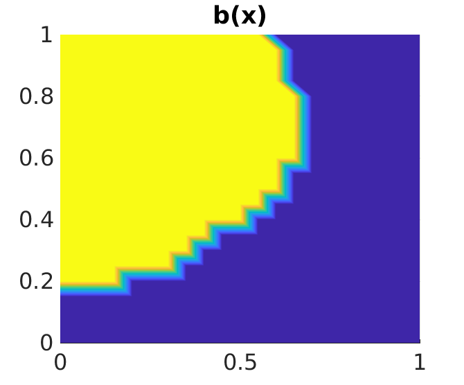


To demonstrate the physical interpretability of the learned kernel, in the first row of Figure 5 we show the ground-truth microstructure , a test loading field instance , and the corresponding solution . By taking the summation of the kernel strength on each row, one can discover the interaction strength of each material point with its neighbors. As this strength is related to the permeability field , the underlying microstructure can be recovered accordingly. In the bottom row of Figure 5, we demonstrate the discovered microstructure of this test task. We note that the discovered microstructure is smoothed out due to the continuous setting of our learned kernel (as shown in the bottom left plot), and a thresholding step is performed to discover the two-phase microstructure. The discovered microstructure (bottom right plot) matches well with the hidden ground-truth microstructure (left plot), except for regions near the domain boundary. This mismatch is due to the applied Dirichlet-type boundary condition ( on ) in all samples, which leads to the measurement pairs containing no information near the domain boundary and makes it impossible to identify the kernel on boundaries.
5.3 Heterogeneous material learning
In this example, we investigate the learning of heterogeneous and nonlinear material responses using the Mechanical MNIST benchmark (Lejeune, 2020). For training and testing, we take 500 heterogeneous material specimens, where each specimen is governed by a Neo-Hookean material with a varying modulus converted from the MNIST bitmap images. On each specimen, 200 loading/response data pairs are provided. Two generalization scenarios are considered. 1) We mix the data from all numbers and randomly take of specimens for testing. This scenario corresponds to an ID test. 2) We leave all specimens corresponding to the number ‘9’ for testing, and use the rest for training. This scenario corresponds to an OOD test. The corresponding results are listed in Table 4, where NAO again outperforms its discrete counterpart, especially in the small-data regime and OOD setting.
| Case | model | #param | ID test | OOD test |
|---|---|---|---|---|
| = 40, =40 | Discrete-NAO | 5,469,528 | 7.21% | 7.95% |
| samples | NAO | 142,534 | 6.57% | 6.26% |
| = 100, =100 | Discrete-NAO | 7,353,768 | 6.34% | 6.01% |
| samples | NAO | 303,814 | 4.75% | 5.58% |
6 Conclusion
We propose Nonlocal Attention Operator (NAO), a novel NO architecture to simultaneously learn both the forward (modeling) and inverse (discovery) solvers in physical systems from data. In particular, NAO learns the function-to-function mapping based on an integral NO architecture and provides a surrogate forward solution predictor. In the meantime, the attention mechanism is crafted in building a kernel map from input-output function pairs to the system’s function parameters, offering zero-shot generalizability to new and unseen physical systems. As such, the kernel map explores in the function space of identifiability, resolving the enduring ill-posedness in inverse PDE problems. In our empirical demonstrations, NAO outperforms all selected baselines on multiple datasets of inverse PDE problems and out-of-distribution generalizability tasks.
Broader Impacts: Beyond its merits in forward/inverse PDE modeling, our work represents an initial exploration in understanding the attention mechanism in physics modeling, and paves a theoretical path towards building a foundation model in scientific ML.
Limitations: Due to limited computational resource, our experiments focus on learning from a small to medium number () of similar physical systems. It would be beneficial to expand the coverage and enable learning across different types of physical systems.
Acknowledgments and Disclosure of Funding
S. Jafarzadeh would like to acknowledge support by the AFOSR grant FA9550-22-1-0197, and Y. Yu would like to acknowledge support by the National Science Foundation (NSF) under award DMS-1753031. Portions of this research were conducted on Lehigh University’s Research Computing infrastructure partially supported by NSF Award 2019035. F. Lu would like to acknowledge support by NSF DMS-2238486.
This article has been authored by an employee of National Technology and Engineering Solutions of Sandia, LLC under Contract No. DE-NA0003525 with the U.S. Department of Energy (DOE). The employee owns all right, title and interest in and to the article and is solely responsible for its contents. The United States Government retains and the publisher, by accepting the article for publication, acknowledges that the United States Government retains a non-exclusive, paid-up, irrevocable, worldwide license to publish or reproduce the published form of this article or allow others to do so, for United States Government purposes. The DOE will provide public access to these results of federally sponsored research in accordance with the DOE Public Access Plan https://www.energy.gov/downloads/doe-public-access-plan.
References
- Besnard et al. (2006) Gilles Besnard, François Hild, and Stéphane Roux. “finite-element” displacement fields analysis from digital images: application to portevin–le châtelier bands. Experimental mechanics, 46(6):789–803, 2006.
- Bucur et al. (2016) Claudia Bucur, Enrico Valdinoci, et al. Nonlocal diffusion and applications, volume 20. Springer, 2016.
- Cai et al. (2022) Shengze Cai, Zhiping Mao, Zhicheng Wang, Minglang Yin, and George Em Karniadakis. Physics-informed neural networks (PINNs) for fluid mechanics: A review. Acta Mechanica Sinica, pages 1–12, 2022.
- Cao (2021) Shuhao Cao. Choose a transformer: Fourier or galerkin. Advances in neural information processing systems, 34:24924–24940, 2021.
- Carleo et al. (2019) Giuseppe Carleo, Ignacio Cirac, Kyle Cranmer, Laurent Daudet, Maria Schuld, Naftali Tishby, Leslie Vogt-Maranto, and Lenka Zdeborová. Machine learning and the physical sciences. Reviews of Modern Physics, 91(4):045002, 2019.
- Chen et al. (2023) Ke Chen, Chunmei Wang, and Haizhao Yang. let data talk: data-regularized operator learning theory for inverse problems. arXiv preprint arXiv:2310.09854, 2023.
- Child et al. (2019) Rewon Child, Scott Gray, Alec Radford, and Ilya Sutskever. Generating long sequences with sparse transformers. arXiv preprint arXiv:1904.10509, 2019.
- Coorey et al. (2022) Genevieve Coorey, Gemma A Figtree, David F Fletcher, Victoria J Snelson, Stephen Thomas Vernon, David Winlaw, Stuart M Grieve, Alistair McEwan, Jean Yee Hwa Yang, Pierre Qian, Kieran O’Brien, Jessica Orchard, Jinman Kim, Sanjay Patel, and Julie Redfern. The health digital twin to tackle cardiovascular disease—A review of an emerging interdisciplinary field. NPJ Digital Medicine, 5:126, 2022.
- Ding et al. (2022) Wen Ding, Kui Ren, and Lu Zhang. Coupling deep learning with full waveform inversion. arXiv preprint arXiv:2203.01799, 2022.
- Dittmer et al. (2020) Sören Dittmer, Tobias Kluth, Peter Maass, and Daniel Otero Baguer. Regularization by architecture: A deep prior approach for inverse problems. Journal of Mathematical Imaging and Vision, 62:456–470, 2020.
- Du et al. (2020) Qiang Du, Bjorn Engquist, and Xiaochuan Tian. Multiscale modeling, homogenization and nonlocal effects: Mathematical and computational issues. Contemporary mathematics, 754:115–140, 2020.
- Fan and Ying (2023) Yuwei Fan and Lexing Ying. Solving traveltime tomography with deep learning. Communications in Mathematics and Statistics, 11(1):3–19, 2023.
- Ferrari and Willcox (2024) Alberto Ferrari and Karen Willcox. Digital twins in mechanical and aerospace engineering. Nature Computational Science, 4(3):178–183, 2024.
- Ghaboussi et al. (1991) J Ghaboussi, JH Garrett Jr, and Xiping Wu. Knowledge-based modeling of material behavior with neural networks. Journal of engineering mechanics, 117(1):132–153, 1991.
- Ghaboussi et al. (1998) Jamshid Ghaboussi, David A Pecknold, Mingfu Zhang, and Rami M Haj-Ali. Autoprogressive training of neural network constitutive models. International Journal for Numerical Methods in Engineering, 42(1):105–126, 1998.
- Goswami et al. (2022) Somdatta Goswami, Aniruddha Bora, Yue Yu, and George Em Karniadakis. Physics-informed neural operators. 2022 arXiv preprint arXiv:2207.05748, 2022.
- Guibas et al. (2021) John Guibas, Morteza Mardani, Zongyi Li, Andrew Tao, Anima Anandkumar, and Bryan Catanzaro. Adaptive fourier neural operators: Efficient token mixers for transformers. arXiv preprint arXiv:2111.13587, 2021.
- Gupta et al. (2021) Gaurav Gupta, Xiongye Xiao, and Paul Bogdan. Multiwavelet-based operator learning for differential equations. Advances in neural information processing systems, 34:24048–24062, 2021.
- Hao et al. (2023) Zhongkai Hao, Zhengyi Wang, Hang Su, Chengyang Ying, Yinpeng Dong, Songming Liu, Ze Cheng, Jian Song, and Jun Zhu. Gnot: A general neural operator transformer for operator learning. In International Conference on Machine Learning, pages 12556–12569. PMLR, 2023.
- He et al. (2021) Qizhi He, Devin W Laurence, Chung-Hao Lee, and Jiun-Shyan Chen. Manifold learning based data-driven modeling for soft biological tissues. Journal of Biomechanics, 117:110124, 2021.
- Ho et al. (2019) Jonathan Ho, Nal Kalchbrenner, Dirk Weissenborn, and Tim Salimans. Axial attention in multidimensional transformers. arXiv preprint arXiv:1912.12180, 2019.
- Jafarzadeh et al. (2024) Siavash Jafarzadeh, Stewart Silling, Ning Liu, Zhongqiang Zhang, and Yue Yu. Peridynamic neural operators: A data-driven nonlocal constitutive model for complex material responses. Computer Methods in Applied Mechanics and Engineering, 425:116914, 2024.
- Jiang et al. (2022) Hanyang Jiang, Yuehaw Khoo, and Haizhao Yang. Reinforced inverse scattering. arXiv preprint arXiv:2206.04186, 2022.
- Karniadakis et al. (2021) George Em Karniadakis, Ioannis G Kevrekidis, Lu Lu, Paris Perdikaris, Sifan Wang, and Liu Yang. Physics-informed machine learning. Nature Reviews Physics, 3(6):422–440, 2021.
- Katharopoulos et al. (2020) Angelos Katharopoulos, Apoorv Vyas, Nikolaos Pappas, and François Fleuret. Transformers are rnns: Fast autoregressive transformers with linear attention. In International conference on machine learning, pages 5156–5165. PMLR, 2020.
- Lai et al. (2019) Ru-Yu Lai, Qin Li, and Gunther Uhlmann. Inverse problems for the stationary transport equation in the diffusion scaling. SIAM Journal on Applied Mathematics, 79(6):2340–2358, 2019.
- Lee-Thorp et al. (2021) James Lee-Thorp, Joshua Ainslie, Ilya Eckstein, and Santiago Ontanon. Fnet: Mixing tokens with fourier transforms. arXiv preprint arXiv:2105.03824, 2021.
- Lejeune (2020) Emma Lejeune. Mechanical mnist: A benchmark dataset for mechanical metamodels. Extreme Mechanics Letters, 36:100659, 2020.
- Li et al. (2022) Zijie Li, Kazem Meidani, and Amir Barati Farimani. Transformer for partial differential equations’ operator learning. arXiv preprint arXiv:2205.13671, 2022.
- Li et al. (2020a) Zongyi Li, Nikola Kovachki, Kamyar Azizzadenesheli, Burigede Liu, Kaushik Bhattacharya, Andrew Stuart, and Anima Anandkumar. Neural operator: Graph kernel network for partial differential equations. arXiv preprint arXiv:2003.03485, 2020a.
- Li et al. (2020b) Zongyi Li, Nikola Kovachki, Kamyar Azizzadenesheli, Burigede Liu, Andrew Stuart, Kaushik Bhattacharya, and Anima Anandkumar. Multipole graph neural operator for parametric partial differential equations. Advances in Neural Information Processing Systems, 33:NeurIPS 2020, 2020b.
- Li et al. (2020c) Zongyi Li, Nikola Borislavov Kovachki, Kamyar Azizzadenesheli, Kaushik Bhattacharya, Andrew Stuart, and Anima Anandkumar. Fourier NeuralOperator for Parametric Partial Differential Equations. In International Conference on Learning Representations, 2020c.
- Li et al. (2021) Zongyi Li, Hongkai Zheng, Nikola Kovachki, David Jin, Haoxuan Chen, Burigede Liu, Kamyar Azizzadenesheli, and Anima Anandkumar. Physics-informed neural operator for learning partial differential equations. 2021 arXiv preprint arXiv:2111.03794, 2021.
- Liu et al. (2021) Hanxiao Liu, Zihang Dai, David So, and Quoc V Le. Pay attention to mlps. Advances in neural information processing systems, 34:9204–9215, 2021.
- Liu et al. (2023) Ning Liu, Yue Yu, Huaiqian You, and Neeraj Tatikola. Ino: Invariant neural operators for learning complex physical systems with momentum conservation. In International Conference on Artificial Intelligence and Statistics, pages 6822–6838. PMLR, 2023.
- Liu et al. (2024a) Ning Liu, Yiming Fan, Xianyi Zeng, Milan Klöwer, LU ZHANG, and Yue Yu. Harnessing the power of neural operators with automatically encoded conservation laws. In Forty-first International Conference on Machine Learning, 2024a.
- Liu et al. (2024b) Ning Liu, Siavash Jafarzadeh, and Yue Yu. Domain agnostic fourier neural operators. Advances in Neural Information Processing Systems, 36, 2024b.
- Liu et al. (2024c) Ning Liu, Xuxiao Li, Manoj R Rajanna, Edward W Reutzel, Brady Sawyer, Prahalada Rao, Jim Lua, Nam Phan, and Yue Yu. Deep neural operator enabled digital twin modeling for additive manufacturing. arXiv preprint arXiv:2405.09572, 2024c.
- Liu et al. (2022) Xinliang Liu, Bo Xu, and Lei Zhang. Ht-net: Hierarchical transformer based operator learning model for multiscale pdes. 2022.
- Lu et al. (2022) Fei Lu, Quanjun Lang, and Qingci An. Data adaptive rkhs tikhonov regularization for learning kernels in operators. In Mathematical and Scientific Machine Learning, pages 158–172. PMLR, 2022.
- Lu et al. (2023) Fei Lu, Qingci An, and Yue Yu. Nonparametric learning of kernels in nonlocal operators. Journal of Peridynamics and Nonlocal Modeling, pages 1–24, 2023.
- Lu et al. (2019) Lu Lu, Pengzhan Jin, and George Em Karniadakis. Deeponet: Learning nonlinear operators for identifying differential equations based on the universal approximation theorem of operators. arXiv preprint arXiv:1910.03193, 2019.
- Lu et al. (2021) Lu Lu, Pengzhan Jin, Guofei Pang, Zhongqiang Zhang, and George Em Karniadakis. Learning nonlinear operators via DeepONet based on the universal approximation theorem of operators. Nature Machine Intelligence, 3(3):218–229, 2021.
- Molinaro et al. (2023) Roberto Molinaro, Yunan Yang, Björn Engquist, and Siddhartha Mishra. Neural inverse operators for solving pde inverse problems. arXiv preprint arXiv:2301.11167, 2023.
- Molnar (2020) Christoph Molnar. Interpretable machine learning. 2020.
- Nekoozadeh et al. (2023) Anahita Nekoozadeh, Mohammad Reza Ahmadzadeh, and Zahra Mardani. Multiscale attention via wavelet neural operators for vision transformers. arXiv preprint arXiv:2303.12398, 2023.
- Obmann et al. (2020) Daniel Obmann, Johannes Schwab, and Markus Haltmeier. Deep synthesis regularization of inverse problems. arXiv preprint arXiv:2002.00155, 2020.
- Ong et al. (2022) Yong Zheng Ong, Zuowei Shen, and Haizhao Yang. IAE-Net: integral autoencoders for discretization-invariant learning. arXiv preprint arXiv:2203.05142, 2022.
- Pfau et al. (2020) David Pfau, James S Spencer, Alexander GDG Matthews, and W Matthew C Foulkes. Ab initio solution of the many-electron schrödinger equation with deep neural networks. Physical Review Research, 2(3):033429, 2020.
- Rao et al. (2021) Yongming Rao, Wenliang Zhao, Zheng Zhu, Jiwen Lu, and Jie Zhou. Global filter networks for image classification. Advances in neural information processing systems, 34:980–993, 2021.
- Rudin et al. (2022) Cynthia Rudin, Chaofan Chen, Zhi Chen, Haiyang Huang, Lesia Semenova, and Chudi Zhong. Interpretable machine learning: Fundamental principles and 10 grand challenges. Statistic Surveys, 16:1–85, 2022.
- Silling (2000) Stewart A Silling. Reformulation of elasticity theory for discontinuities and long-range forces. Journal of the Mechanics and Physics of Solids, 48(1):175–209, 2000.
- Sun et al. (2024) Jingmin Sun, Yuxuan Liu, Zecheng Zhang, and Hayden Schaeffer. Towards a foundation model for partial differential equation: Multi-operator learning and extrapolation. arXiv preprint arXiv:2404.12355, 2024.
- Tolstikhin et al. (2021) Ilya O Tolstikhin, Neil Houlsby, Alexander Kolesnikov, Lucas Beyer, Xiaohua Zhai, Thomas Unterthiner, Jessica Yung, Andreas Steiner, Daniel Keysers, Jakob Uszkoreit, et al. Mlp-mixer: An all-mlp architecture for vision. Advances in neural information processing systems, 34:24261–24272, 2021.
- Touvron et al. (2022) Hugo Touvron, Piotr Bojanowski, Mathilde Caron, Matthieu Cord, Alaaeldin El-Nouby, Edouard Grave, Gautier Izacard, Armand Joulin, Gabriel Synnaeve, Jakob Verbeek, et al. Resmlp: Feedforward networks for image classification with data-efficient training. IEEE Transactions on Pattern Analysis and Machine Intelligence, 45(4):5314–5321, 2022.
- Tsai et al. (2019) Yao-Hung Hubert Tsai, Shaojie Bai, Makoto Yamada, Louis-Philippe Morency, and Ruslan Salakhutdinov. Transformer dissection: a unified understanding of transformer’s attention via the lens of kernel. arXiv preprint arXiv:1908.11775, 2019.
- Uhlmann (2009) Gunther Uhlmann. Electrical impedance tomography and calderón’s problem. Inverse problems, 25(12):123011, 2009.
- Vaswani et al. (2017) Ashish Vaswani, Noam Shazeer, Niki Parmar, Jakob Uszkoreit, Llion Jones, Aidan N Gomez, Łukasz Kaiser, and Illia Polosukhin. Attention is all you need. Advances in neural information processing systems, 30, 2017.
- Wang et al. (2020) Sinong Wang, Belinda Z Li, Madian Khabsa, Han Fang, and Hao Ma. Linformer: Self-attention with linear complexity. arXiv preprint arXiv:2006.04768, 2020.
- Wei and Zhang (2023) Min Wei and Xuesong Zhang. Super-resolution neural operator. In Proceedings of the IEEE/CVF Conference on Computer Vision and Pattern Recognition, pages 18247–18256, 2023.
- Xu et al. (2019) Zhi-Qin John Xu, Yaoyu Zhang, Tao Luo, Yanyang Xiao, and Zheng Ma. Frequency principle: Fourier analysis sheds light on deep neural networks. arXiv preprint arXiv:1901.06523, 2019.
- Yang and Osher (2024) Liu Yang and Stanley J Osher. Pde generalization of in-context operator networks: A study on 1d scalar nonlinear conservation laws. arXiv preprint arXiv:2401.07364, 2024.
- Yang et al. (2021) Liu Yang, Xuhui Meng, and George Em Karniadakis. B-pinns: Bayesian physics-informed neural networks for forward and inverse pde problems with noisy data. Journal of Computational Physics, 425:109913, 2021.
- Ye et al. (2024) Zhanhong Ye, Xiang Huang, Leheng Chen, Hongsheng Liu, Zidong Wang, and Bin Dong. Pdeformer: Towards a foundation model for one-dimensional partial differential equations. arXiv preprint arXiv:2402.12652, 2024.
- Yilmaz (2001) Özdoğan Yilmaz. Seismic data analysis, volume 1. Society of exploration geophysicists Tulsa, 2001.
- You et al. (2021) Huaiqian You, Yue Yu, Nathaniel Trask, Mamikon Gulian, and Marta D’Elia. Data-driven learning of nonlocal physics from high-fidelity synthetic data. Computer Methods in Applied Mechanics and Engineering, 374:113553, 2021.
- You et al. (2022) Huaiqian You, Yue Yu, Marta D’Elia, Tian Gao, and Stewart Silling. Nonlocal kernel network (NKN): A stable and resolution-independent deep neural network. Journal of Computational Physics, page arXiv preprint arXiv:2201.02217, 2022.
- Zhang et al. (2018) Linfeng Zhang, Jiequn Han, Han Wang, Roberto Car, and E Weinan. Deep potential molecular dynamics: a scalable model with the accuracy of quantum mechanics. Physical Review Letters, 120(14):143001, 2018.
- Zhang (2024) Zecheng Zhang. Modno: Multi operator learning with distributed neural operators. arXiv preprint arXiv:2404.02892, 2024.
Appendix A Riemann sum approximation derivations
In this section, we show that the discrete attention operator (6) can be seen as the Riemann sum approximation of the nonlocal attention operator in (15), in the continuous limit. Without loss of generality, we consider a uniform discretization with grid size . Denoting the th layer output as , , and as , for the th () layer update in (6) writes:
That means, only controls the rank bound when lifting each point-wise feature via , while characterizes the (trainable) interaction of input function pair instances. Moreover, when , . When , . Then,
Similarly,
With the Riemann sum approximation: , one can further reformulate above derivations as:
Therefore, the attention mechanism of each layer is in fact an integral operator after a rescaling:
| (27) |
with the kernel defined as:
| (28) |
For the th layer update, we denote the approximated value of as , then
Hence, a (rescaled) continuous limit of the kernel writes:
Appendix B Proofs and connection with regularized estimator
B.1 Proofs
Proof of Lemma 4.2.
The proof is adapted from Lu et al. (2023, 2022). Write . Notice that the loss function in (16) can be expanded as
where is the integral operator
and is the Riesz representation of the bounded linear functional
Thus, the quadratic loss function has a unique minimizer in .
Meanwhile, since the data pairs are continuous with compact support, the function is a square-integrable reproducing kernel. Thus, the operator is compact and . Then, , where the closure is with respect to . ∎
B.2 Connection with regularized estimator
Consider the inverse problem of estimating the nonlocal kernel given a data pair . In the classical variational approach, one seeks the minimizer of the following loss function
| (30) |
The inverse problem is ill-posed in the sense that the minimizer can often be non-unique or sensitive to the noise or measurement error in data . Thus, regularization is crucial to produce a stable solution.
To connect with the attention-based model, we consider regularizing using an RKHS with a square-integrable reproducing kernel . One seeks an estimator in by regularizing the loss with the , and minimizes the regularized loss function
| (31) |
The next lemma shows that the regularized estimator is a nonlinear function of the data pair , where the nonlinearity comes from the kernel and the parameter .
Lemma B.1.
When there is no prior information on the regularization, which happens often for the learning of the kernel, one can use the data-adaptive RKHS with the reproducing kernel determined by data:
| (34) |
Lu et al. (2023) shows that this regularizer can lead to consistent convergent estimators.
Remark B.2 (Discrete data and discrete inverse problem).
In practice, the datasets are discrete. One can view the discrete inverse problem as a discretization of the continuous inverse problem. Assume that the integrands are compactly supported and when the integrals are approximated by Riemann sums, we can write loss function for discrete as
| (35) |
where, recalling the definition of the token in (5),
and .
The minimizer of this discrete loss function with the optimal hyper-parameter is
In particular, when taking and using the Neumann series , we have
In particular, depends on both and . Hence, the estimator is nonlinear in and , and it is important to make the attention depend nonlinearly on the token , as in (7).
Proof of Lemma B.1.
Since is radial and noticing that
since , we can write
Meanwhile, by the Riesz representation theorem, there exists a function such that
Combining these two equations, we can write the loss function as
Then, we can write the regularized loss function as
Selecting the optimal hyper-parameter , which depends on both and , and setting the Fréchet derivative of over to be zero, we obtain the regularized estimator in (33). ∎
Appendix C Data generation and additional discussion
C.1 Example 1: radial kernel learning
In all settings except the “single task” one, all kernels act on the same set of functions with and . In the “single task” setting, to create more diverse samples, the single kernel acts on a set of 14 functions: , and , . In the ground-truth model, the integral is computed by the adaptive Gauss-Kronrod quadrature method, which is much more accurate than the Riemann sum integrator that we use in the learning stage. To create discrete datasets with different resolutions, for each , we take values , where is the grid point on the uniform mesh of size . We form a training sample of each task by taking pairs from this task. When taking the token size and function pairs, each task contains samples.
C.2 Example 2: solution operator learning
For one example, we generate the synthetic data based on the Darcy flow in a square domain of size subjected to Dirichlet boundary conditions. The problem setting is: subjected to on all boundaries. This equation describes the diffusion in heterogeneous fields, such as the subsurface flow of underground water in porous media. The heterogeneity is represented by the location-dependent conductivity . is the source term, and the hydraulic height is the solution. For each data instance, we solve the equation on a grid using an in-house finite difference code. We consider 500 random microstructures consisting of two distinct phases. For each microstructure, the square domain is randomly divided into two subdomains with different conductivity of either 12 or 3. Additionally, we consider 100 different functions obtained via a Gaussian random field generator. For each microstructure, we solve the Darcy problem considering all 100 source terms, resulting in a dataset of function pairs in the form of , and where ’s are the discretization points on the square domain.
In operator learning settings, we note that the permutation of function pairs in each sample should not change the learned kernel, i.e., one should have , where is the permutation operator. Hence, we augment the training dataset by permuting the function pairs in each task. Specifically, with microstructures (tasks) and function pairs per task, we randomly permut the function pairs and take function pairs for times per task. As a result, we can generate a total of 10000 samples (9000 for training and 1000 for testing) in the form of .
C.3 Example 3: heterogeneous material learning
In the Mechanical MNIST dataset, we generate a large set of heterogeneous material responses subjected to mechanical forces. This is similar to the approach in Lejeune (2020). The material property (stiffness) of the heterogeneous medium is constructed assuming a linear scaling between 1 and 100, according to the gray-scale bitmap of the MNIST images, which results in a set of 2D square domains with properties that vary according to MNIST digit patterns. The problem setting for this data set is the equilibrium equation: subjected to Dirichlet boundary condition of zero displacement and nonzero variable external forces:. is the stress tensor and is a nonlinear function of displacement . The choice of material models determines the stress function, and here we employ the Neo-Hookean material model as in Lejeune (2020). From MNIST, we took 50 samples of each digit resulting in a total of 500 microstructures. We consider 200 different external forces obtained via a Gaussian random field, and solve the problem for each pair of microstructure and external force, resulting in samples. To solve each sample, we use FEniCS finite element package considering a uniform mesh. We then downsample from the finite element nodes to get values for the solution and external force on a the coarser equi-spaced grid. The resulting dataset is of the form: , and where ’s are the equi-spaced sampled spatial points.
Similar to Example 2, we perform the permutation trick to augment the training data. In particular, with microstructures (tasks) and function pairs per task, we randomly permute the function pairs and take function pairs for times per task. As a result, we can generate a total of 50000 samples, where 45000 are used for training and 5000 for testing.
Appendix D Computational complexity
Denote as the size of the spatial mesh, the number of data pairs in each training model, the column width of the query/key weight matrices and , the number of layers, and the number of training models. The number of trainable parameters in a discrete NAO is of size . For continuous-kernel NAO, taking a three-layer MLP as a dense net of size for the trainable kernels and for example, its the corresponding number of trainable parameters is . Thus, the total number of trainable parameters for a continuous-kernel NAO is .
The computational complexity of NAO is quadratic in the length of the input and linear in the data size, with flops in each epoch in the optimization. It is computed as follows for each layer and the data of each training model: the attention function takes flops, and the kernel map takes flops; thus, the total is flops. In inverse PDE problems, we generally have , and hence the complexity of NAO is per layer per sample.
Compared with other methods, it is important to note that NAO solves both forward and ill-posed inverse problems using multi-model data. Thus, we don’t compare it with methods that solve the problems for a single model data, for instance, the regularized estimator in Appendix B. Methods solving similar problems are the original attention model (Vaswani et al., 2017), convolution neural network (CNN), and graph neural network (GNN). As discussed in Vaswani et al. (2017), these models have a similar computational complexity, if not any higher. In particular, the complexity of the original attention model is , and the complexity of CNN is with being the kernel size, and a full GNN is of complexity .