2025 \startpage1
Nonlinear receding-horizon differential game for drone racing along a three-dimensional path
Toshiyuki Ohtsuka, Department of Informatics, Graduate School of Informatics, Kyoto University, Kyoto 606-8501, Japan. Email: [email protected]
Nonlinear receding-horizon differential game for drone racing along a three-dimensional path
Abstract
[Abstract]Drone racing involves high-speed navigation of three-dimensional paths, posing a substantial challenge in control engineering. This study presents a game-theoretic control framework, the nonlinear receding-horizon differential game (NRHDG), designed for competitive drone racing. NRHDG enhances robustness in adversarial settings by predicting and countering an opponent’s worst-case behavior in real time. It extends standard nonlinear model predictive control (NMPC), which otherwise assumes a fixed opponent model. First, we develop a novel path-following formulation based on projection point dynamics, eliminating the need for costly distance minimization. Second, we propose a potential function that allows each drone to switch between overtaking and obstructing maneuvers based on real-time race situations. Third, we establish a new performance metric to evaluate NRHDG with NMPC under race scenarios. Simulation results demonstrate that NRHDG outperforms NMPC in terms of both overtaking efficiency and obstructing capabilities.
keywords:
drone control, path following, differential game, model predictive control1 Introduction
Drone racing is an emerging field in robotics that requires drones to navigate three-dimensional paths at high speeds with precision.1 These races pose significant control challenges, requiring trajectory adjustments under nonlinear dynamics. Although recent advances in trajectory optimization have enabled precise gate passages and energy-efficient maneuvers,2 existing methods have predominantly focused on single-drone scenarios. Similarly, learning-based approaches can navigate moving gates;3 however, they often overlook the multi-agent competitive interactions.
To address these competitive interactions, several studies4, 5, 6 have formulated drone racing as receding-horizon differential games (RHDG). Unlike standard model predictive control (MPC), RHDG predicts the opponent’s worst-case actions over a finite horizon, thus optimizing the ego drone’s strategy accordingly. In particular, the nonlinear receding-horizon differential game (NRHDG) 6 handles fully nonlinear dynamics, rather than relying on simplified kinematic models.4, 5 However, this approach still assumes fixed roles (i.e., overtaking or obstructing) for each drone, limiting the ability to switch strategies during a race. Moreover, relying on explicit path features, such as curvature and torsion, can increase computational costs and lead to potential numerical singularities.
In this study, we enhance the conventional NRHDG framework to facilitate dynamic role-switching and reduce reliance on cumbersome path information. Furthermore, we introduce a novel path-following model that integrates seamlessly with the drone’s state equation without iterative minimization, and we devise a potential function that allows each drone to flexibly move between overtaking and obstructing modes in real time. Finally, we introduce a systematic performance metric to evaluate NRHDG with standard nonlinear MPC (NMPC). Simulation results confirm that NRHDG outperforms NMPC in both overtaking efficiency and obstructing performance along a three-dimensional path.
The main contributions of this work can be summarized as follows.
-
1.
We derive a unified dynamical model for projection onto a three-dimensional path. Unlike existing formulations requiring distance minimization or frame-specific parameters, our model embeds directly into the drone’s state equation and applies to any smooth curve of arbitrary dimension.
-
2.
We propose a custom potential function for NRHDG that enables real-time switching between overtaking and obstructing strategies, adapting to each drone’s relative position.
-
3.
We introduce a performance metric for evaluating the effectiveness of overtaking and obstructing in drone racing. Numerical simulations demonstrate that NRHDG outperforms NMPC.
The first contribution of the above offers a unified and computationally efficient framework for path-following control,7, 8, 9 one of the practically important problems in control engineering. Conventional path-following control methods involve iterative searches or approximations of an orthogonal projection (a projection point) of the vehicle’s position to the path 10, 11, 12, 13, 14 or are limited to two-dimensional paths.15, 16 Other methods define reference points on the path arbitrarily by geometric relationships 17, 18, 19, 20 such as carrot chasing or timing laws 21, 22 as additional degrees of freedom. Furthermore, there are different settings of path-following control based on implicit function representations of paths 23, 24, 25 or vector fields.26 However, arbitrary reference points do not represent the actual distance from the path, and implicit function representations and vector fields are often difficult to construct and apply in general. In contrast, the proposed dynamical model of the projection point provides a computationally efficient and unified formulation for path-following control, making it particularly suited for dynamic and complex environments such as drone racing.
The remainder of this paper is organized as follows. In Section 2, we derive dynamical models of a drone and projection of the drone’s position onto a three-dimensional path. In Section 3, we give an overview of NMPC and NRHDG. In Section 4, we propose objective functions for NMPC and NRHDG, including a potential function for role-switching. In Section 5, we introduce a performance metric to evaluate controllers and perform numerical simulations of races along a three-dimensional path, demonstrating the advantages of NRHDG over NMPC. Finally, in Section 6, we state the conclusions of this study and discuss future work.
2 Modeling
2.1 Dynamics of drone
In this section, we consider a quadrotor-type drone whose dynamical model is derived from reference.27 The inertial frame is denoted by , and the body frame by with origin at the drone’s center of mass, as shown in Figure 1. Attitude is parameterized by the quaternion28 . The rotation matrix from the body frame to the inertial frame is formed as follows:
| (1) |
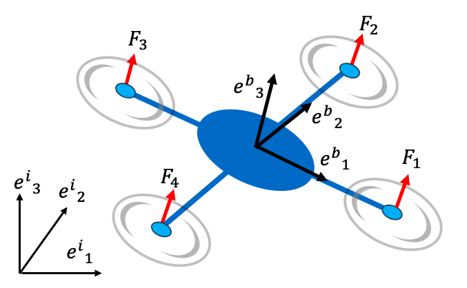
We assume that the external forces acting on the drone consist only of gravity in the direction and rotor thrusts in the direction, and each rotor generates a reaction torque that is proportional to its thrust. Then, the Newton-Euler equations describing translational motion in the inertial frame and rotational motion in the body frame for the drone are expressed as follows.
| (2) |
where represents the drone’s position in the inertial frame, is the angular velocity vector in the body frame, and is the vector of rotor thrusts. Symbols and are the mass and inertia matrix of the drone, respectively, denotes the third column of , , and is a matrix
| (3) |
with the distance from the center of mass to each rotor, and the proportion constant relating thrust to reaction toque. The time derivative of the quaternion is given by
| (4) |
where is the following skew-symmetric matrix
| (5) |
We now define the 13-dimensional state vector . Combining Eqs. (2) and (4), the state equation for the drone is given as follows:
| (6) |
2.2 Dynamics of projection point and arc length
Subsequently, in this section, we analyze the relationship between the drone’s position and the path it should follow. By formulating the dynamics of a projection point and its associated arc length, we establish a foundation for efficient path-following control. We assume that the path is given as a curve parameterized by a path parameter over an interval . That is, the path is represented as the image of a mapping . We assume is twice differentiable and the tangent vector does not vanish for any , which guarantees that does not move backwards when increases. However, we do not assume that the mapping is one-to-one globally, allowing the path to go through a point multiple times. The path parameter is not necessarily the arc length of the path, which allows us to have explicit representations of various paths.
We define the distance from the drone’s position to the path by the minimum distance as
| (7) |
If this infimum is attained at in the interior of , then the stationary condition
| (8) |
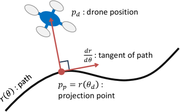
holds. For satisfying (8), we call a point a projection point of because (8) implies that is an orthogonal projection of onto the path, as shown in Figure 2. We also define the signed arc length from to along the path as
| (9) |
for , which is negative when . If the trajectory of the drone is differentiable in time , we can derive ordinary differential equations for and the corresponding arc length .
Theorem 2.1.
Suppose the path is twice differentiable with for any , and the trajectory of the drone is differentiable for any . If is a solution of a differential equation
| (10) |
with its initial value satisfying (8), and
| (11) |
holds for any , then is a projection point with a local minimum distance from the drone’s position for all . Moreover, the arc length of the projection point along the path satisfies a differential equation
| (12) |
for all with the initial condition .
Proof 2.2.
We obtain (10) by differentiating (8) with respect to time. In other words, (10) implies that the time derivative of the left-hand side of (8) is identically zero. Since the left-hand side of (8) is equal to zero at by the assumption on the initial value , it remains zero for all provided that (10) holds. Moreover, (11) implies that the second-order derivative of with respect to is always positive for and for all . Therefore, (8) and (11) imply that is a local minimizer of for each . Note that the sufficient conditions for a local minimizer are valid even when is at the boundary of .29 Finally, by differentiating with respect to time, we obtain (12) and observe that by definition.
Remark 2.3.
Theorem 2.1 ensures that the path parameter and the arc length of the projection point can be computed dynamically by integrating differential equations (10) and (12), without requiring iterative search or approximation in conventional methods.10, 11, 12, 13, 14 This formulation simplifies path-following control by eliminating computational overhead while maintaining generality across three-dimensional paths. It also does not involve specific frames along the path, such as the Frenet-Serret frame, and is applicable to any dimension, in contrast to the other existing methods.15, 16
Remark 2.4.
The singularity in the differential equations (10) and (12) occurs when the denominator of (10) vanishes, which is avoided if
| (13) |
holds, that is, if the deviation or the curvature of the path is sufficiently small. Moreover, Theorem 2.1 also guarantees the local minimum distance of the projection point if the singularity does not occur, which is the best possible guarantee without global search.
2.3 Augmented state equation for path following
To incorporate path-following dynamics into the drone’s control framework, we augment the state vector of the drone with the path parameter and the arc length . This extension enables seamless integration of path-following errors into the control design without requiring additional optimization steps. Specifically, since the right-hand sides of the differential equations Eqs. (10) and (12) depend on , , and , we can integrate them into the state equation of the drone. Subsequently, by augmenting the state vector as , we obtain the augmented state equation for path following as follows:
| (14) |
Equation (14) defines the augmented state equation for the drone, including the dynamics of the projection point () and the associated arc length (). The additional terms allow the control system to directly account for path-following errors in real-time decision-making.
3 Control methods
In competitive drone racing, the control system must address both the drone’s nonlinear dynamics and potential adversarial behavior from an opponent. This section discusses two suitable approaches, which are NMPC and NRHDG.
3.1 Nonlinear model predictive control
In this section, we first review NMPC, a widely used real-time optimization-based control approach for nonlinear systems, in a continuous-time setting.30 We consider a dynamical system
| (15) |
where is the state and is the control input. To determine the control input at each time instant, NMPC solves a finite-horizon optimal control problem (OCP) to minimize the following objective function with a receding horizon .
| (16) |
where and represent the predicted state and control input over the horizon, respectively. They may not necessarily coincide with the actual system’s state and control input in the future.
At each time , the initial value of the optimal control input minimizing the objective function (16) over the horizon is used as the actual control input for that time. Subsequently, NMPC defines a state feedback control law because the control input depends on the current state of the system that is used as the initial state in the OCP over . NMPC can handle various control problems if the OCP is solved numerically in real time. However, it cannot handle multi-agent interactions in competitive scenarios such as drone racing. This limitation arises from the need to predict the opponent’s behavior, which is inherently uncertain. Therefore, NMPC requires simplifying assumptions about the opponent’s future trajectory, reducing its effectiveness in adversarial environments.
3.2 Nonlinear receding-horizon differential game
To explicitly model an adversarial opponent, we employ NRHDG, an extension of NMPC incorporating a differential game problem (DGP).31 In what follows, we limit our discussion to a two-player zero-sum DGP, where one player’s gain is exactly the other player’s loss, making it a suitable model for competitive scenarios. We consider a dynamical system described by a state equation
| (17) |
where is the combined state of two players, is the strategy (control input) for player , and is the strategy for player . One player aims to minimize some objective function, while the other aims to maximize it. We assume that both players know the current state of the game and the state equation governing the game.
In NRHDG, we consider an objective function with a receding horizon as follows:
| (18) |
which models the zero-sum nature of the game. If there exists a pair of strategies such that
| (19) |
holds for any strategies and , is called a saddle-point solution. The saddle-point solution ensures that both players adopt optimal strategies, balancing minimization by player and maximization by player . In particular, the player can achieve a lower value of the objective function if chooses a different strategy from . Therefore, can use the initial value of a saddle-point solution for the DGP as the actual input to the system regardless of the control input of , which also defines a state feedback control law for . This property makes NRHDG suitable for dynamic problems in competitive scenarios such as drone racing. Although the necessary conditions for a saddle-point solution of a DGP are identical to the stationary conditions for an OCP,31 numerical solution methods for NMPC are not necessarily applicable to NRHDG if they are tailored for minimization, for instance, involving line searches. However, there are some methods that are applicable to both NMPC and NRHDG.6, 32, 33
4 Design of objective functions for competitive drone racing
4.1 Control objectives
This section describes the construction of the objective functions for NMPC and NRHDG that balance the following two key racing objectives.
-
1.
Path following: Ensure that the drone progresses efficiently along the predefined three-dimensional path, minimizing deviations while allowing flexibility for dynamic maneuvers. This flexibility avoids strict convergence to the path, which can hinder competitive behaviors such as overtaking or obstructing.
-
2.
Overtaking and obstructing: Enable the ego drone to dynamically switch between overtaking a preceding opponent and obstructing a following opponent, depending on the race scenario. These behaviors are achieved while ensuring collision avoidance and maintaining competitive efficiency.
We first design an objective function for NMPC to achieve the above objectives. Subsequently, we modify it to define an objective function for NRHDG.
4.2 NMPC objective function
4.2.1 Path-following term
Consider the augmented drone state in Section 2, which includes position , velocity , angular velocity , quaternion , path parameter , and arc length . We define a stage cost for path following as follows:
| (20) |
where represents the reference input when the drone is in a hovering state. The parameters represent the state weights, while serves as the input weight. The stage cost in (20) balances multiple objectives for path following: The first term penalizes deviations from the desired path. The second term penalizes the drone’s angular velocity to suppress excessive attitude motion. The third term maximizes the drone’s progress along the path. The final term suppresses large deviations in the control inputs from the reference input. A corresponding terminal cost
| (21) |
ensures the terminal state aligns with the path-following objective. Since the path parameter and the arc length of the projection point are embedded in the state equation as state variables, the stage and terminal costs do not involve any optimization problem nor complicated coordinate transformation to determine the projection point for a wide class of three-dimensional paths.
4.2.2 Overtaking and obstructing term
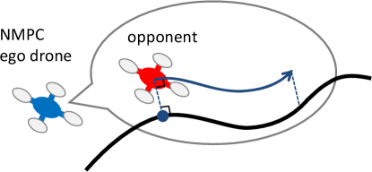
To enable the ego drone to overtake or obstruct an opponent, we introduce a potential function that depends on both the ego-drone’s state and the opponent’s predicted state. For NMPC, we assume that the opponent moves at a constant speed in parallel to the path (Figure 3). Specifically, the ego drone predicts the position and path parameter of the opponent by a simplified state equation
| (22) |
where denotes the constant speed of the opponent. We denote the state vector of the simplified prediction model as .
Here, we define a potential function for overtaking and obstructing in NMPC as follows.
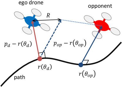
| (23) | ||||
| (24) |
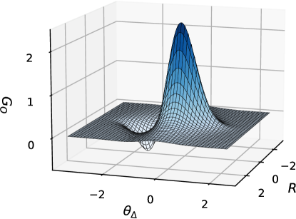
where represents the difference of the path parameters between the ego drone and the opponent, represents the difference in the deviations of the two drones from the path (Figure 4), and , , , , and are constants. The shape of this potential function is shown on the - plane in Figure 5, where the origin corresponds to the location of the ego drone. The potential function in (23) enables adaptive overtaking and obstructing behaviors based on the relative position of the ego drone to its opponent. When is positive, the ego drone follows the opponent and should avoid and overtake the opponent. Therefore, we define the potential function such that it has its maximum at when is positive. Here, we use , the difference in the deviations of the two drones from the path, rather than the distance , because does not depend on the distance of the two drones along the path. That is, the ego drone does not slow down to keep the distance from the opponent along the path when it avoids and overtakes the opponent. However, when is negative, the ego drone precedes the opponent and should obstruct the opponent not to be overtaken. To induce obstructing behavior, the potential function has its minimum at when is negative. Since is independent of the distance of the two drones along the path, the ego drone maintains its speed when obstructing the opponent.
4.2.3 Overall NMPC cost
In this section, we formulate NMPC for drone racing and define the overall objective function. The ego drone predicts its future motions and the opponent using state equations (14) and (22), and the state vector of the entire system is defined as . Subsequently, we define the stage cost and terminal cost of NMPC by combining the objective functions for path following and overtaking and obstructing, which enables the ego drone to balance path following with competitive behaviors, as follows.
| (25) | |||
| (26) |
These costs determine behaviors of the ego drone depending on the race scenario represented by the states of the two drones. In particular, since the path parameters and are components of the state vectors determined by the state equations (14) and (22), there is no need for additional optimization or moving frames to determine the projection point along the path, which makes the proposed formulation advantageous over conventional formulations of path-following control.
4.3 NRHDG objective function
In NRHDG, the ego drone minimizes an objective function (18) while assuming that the opponent maximizes the same objective function. Furthermore, the ego drone assumes that the opponent is also governed by the same augmented state equation (14). Unlike NMPC, which assumes a fixed prediction model for the opponent, NRHDG explicitly models the opponent’s strategy as a dynamic, adversarial behavior. By incorporating a zero-sum game framework, NRHDG enables the ego drone to optimize its performance against the opponent that actively counters its actions. We denote the state vector and the input vector of the opponent by and , respectively, which consist of the opponent’s variables corresponding to those of and . We also denote the state vector of the entire system as . We now define the stage cost and the terminal cost for NRHDG as
| (27) | ||||
| (28) |
The stage cost in (27) includes terms for both the ego drone and the opponent, reflecting the adversarial nature of the interaction. The terminal cost in (28) evaluates the terminal state of the game, ensuring that each drone’s strategy aligns with the race objectives. These costs create a zero-sum strategic behaviors where the ego drone minimizes its cost while maximizing the opponent’s. At each time , the ego drone determines its control input by solving the NRHDG problem subject to the 30-dimensional state equation for .
5 Performance evaluation in competitive scenarios
5.1 Performance metric
This section assesses the effectiveness of the proposed NRHDG compared to the baseline NMPC in competitive drone racing scenarios. We focus on the following two key aspects.
-
1.
Overtaking performance: The ability of the following drone to maximize its progress while overtaking the preceding drone.
-
2.
Obstructing performance: The ability of the preceding drone to minimize the following drone’s progress while being overtaken.
These metrics reflect both offensive (overtaking) and defensive (obstructing) capabilities of the controllers in adversarial races. For notation, we label NMPC as controller and NRHDG as controller . In a race denoted by , the drone using controller starts ahead, while the drone using controller starts behind.
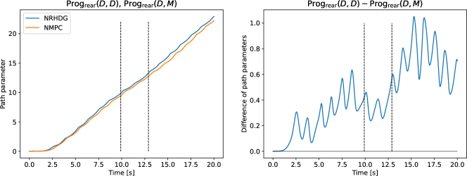
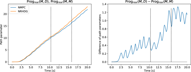
To evaluate the overtaking performance, we compare each pair of two races, and , for . This means that we set the leading controller to be the same in both races and compare the progress of the drone starting from the rear position. To compare controllers fairly, the race settings, such as the initial lead and weight coefficients in the objective functions, are set to be the same between both races. Moreover, the race settings are chosen so that the controller starting from the rear position eventually overtakes the opponent starting ahead in all races, which enables us to make a quantitative comparison between different controllers in different races. The controller achieving more progress while overtaking against the same controller has better overtaking performance. Here, we measure the progress of a drone by its path parameter and define a symbol, , to represent the progress of controller at a certain time in . A larger value of indicates better overtaking performance by the rear-position drone (controller ). That is, if the relationship holds most of the time in both races, makes its progress more effectively than and has better overtaking performance than . Since NRHDG (controller ) explicitly models the opponent’s behavior and optimizes against the worst-case scenarios, it will outperform NMPC (controller ). Therefore, we can expect NRHDG to have better overtaking performance than NMPC as follows.
| (29) |
which means NRHDG (controller ) achieves more progress than NMPC (controller ) when overtaking the same controller .
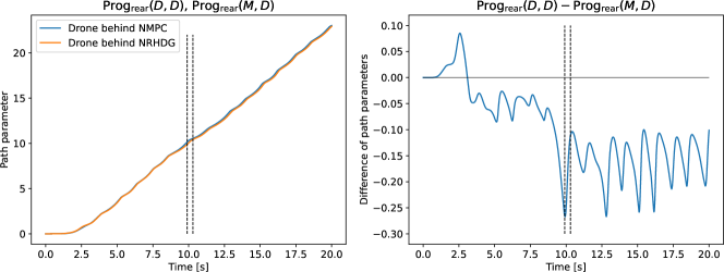
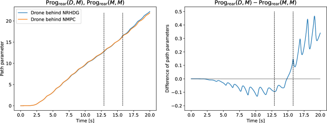
A similar discussion can be made for obstructing performance. To evaluate obstructing performance, we compare each pair of two races, and for . This implies that we set the controller starting from the rear position to the same in two races and observe the difference between the two races. Specifically, the controller that more effectively slows the progress of the rear-position drone has better obstructing performance. Therefore, a lower value of indicates better obstructing performance of the front-position drone (controller ). That is, if the relationship holds most of the time in the two races, obstructs the progress of more effectively than and has better obstructing performance than . Therefore, the following relationship should hold between NRHDG (controller ) and NMPC (controller ).
| (30) |
which means NRHDG obstructs the progress of controller better than NMPC.
Subsequently, the relationships in (29) and (30) imply
| (31) | ||||
| (32) |
where the first and second inequalities in (31) are obtained from (29) and (30), respectively, with , and those in (32) are obtained from (30) and (29), respectively, with . Finally, (31) and (32) imply
| (33) |
If the relationships in (29) and (30) or (31)–(33) hold in numerical simulations, NRHDG is more suitable for drone racing than NMPC.
5.2 Race setup
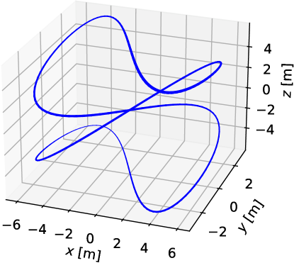
We simulate races on a three-dimensional path
| (35) |
depicted in Figure 6. This path tests the controllers’ ability to handle complex three-dimensional environments with varying curvature and torsion. The sinusoidal path includes sharp turns and gradual slopes, challenging the drones’ path-following and maneuvering capabilities. The rear drone starts at , and the front drone starts at . The physical parameters of the drones in the simulation are shown in Table 1, which are based on the Parrot MamboFly platform.34 The weight coefficients and constants in the objective functions of NMPC and NRHDG are shown in Table 2. We assigned different input weights to represent a speed advantage for the rear drone () and a slower response for the front drone ().
| Variable | Meaning | Value |
|---|---|---|
| Mass of the aircraft | 0.063 kg | |
| Gravitational acceleration | 9.81 m/ | |
| Distance from the center of mass to the rotor | 0.0624 m | |
| Moment of inertia around the roll axis | ||
| Moment of inertia around the pitch axis | ||
| Moment of inertia around the yaw axis | ||
| Proportional constant between reaction torque and thrust | 0.0024 m |
| Parameter | Value |
|---|---|
| 1 | |
| 0.1 | |
| 0.5 | |
| 1 | |
| 4 | |
| 5 | |
We implemented NRHDG and NMPC with a continuation-based real-time optimization algorithm, C/GMRES,35 and its automatic code generation tool, AutoGenU for Jupyter.36†††https://ohtsukalab.github.io/autogenu-jupyter The C/GMRES finds a stationary solution to an optimal control problem without any line searches and is also applicable directly to NRHDG problems. AutoGenU for Jupyter generates C++ code and a Python package for updating the solution with C/GMRES. Then, those codes for NRHDG and NMPC can be used together for simulation of drone racing. We conducted numerical simulations on a PC (CPU: Core i9-12900 2.4 GHz, RAM: 16 GB, OS: Ubuntu 22.04.2 LTS on WSL2, hosted by Windows 11 Pro) to demonstrate the feasibility of real-time implementation. The simulation ran for 20 s, with a horizon length of 0.4 s and a control cycle of 1 ms. The average computation times per update were 0.8 ms for NRHDG and 0.5 ms for NMPC, both of which are within the control cycle.
5.3 Simulation results
5.3.1 Time histories and example overtaking scenario
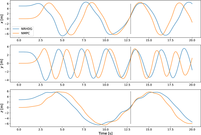
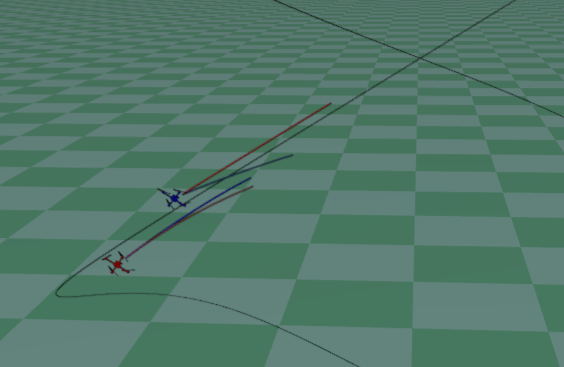
Figure 7 shows a sample time history from , where controller (NRHDG) starts ahead and controller (NMPC) starts behind. The dashed vertical line indicates the moment manages to overtake . The altitudes () of the two drones oscillate as they attempt to obstruct or overtake one another. Figure 8 shows a snapshot of around the overtaking time. The blue drone (NRHDG) predicts its future trajectory and that of the opponent, which are shown as the blue trajectories, while the red trajectories represent the predictions by the red drone (NMPC). NRHDG generates its blue trajectory moving toward the front of the red drone, while NMPC predicts the blue drone to move in parallel to the path. Moreover, NRHDG predicts the red drone to move in parallel to the path, while NMPC generates a larger avoidance motion than NRHDG’s prediction. This indicates that NRHDG generates a less conservative prediction regarding the opponent’s future behavior compared to NMPC.
5.3.2 Comparisons across multiple races
Overtaking performance
First, we evaluate the overtaking performance by comparing two races: and with . The comparison of and for is shown in Figure 9 in terms of the progress of the drone starting from the rear position. Two vertical lines indicate the overtaking times in the two races. After overtaking, the two drones do not interact. Therefore, we focus on the plots from the start time to the overtaking time. In Figure 9, the figure on the left shows the plots of and , and the figure on the right shows their difference, . As can be seen in the figure on the right, exceeds between the start time and the overtaking time. That is, NRHDG makes more progress than NMPC while overtaking the same opponent . The comparison of and for is shown in Figure 9. As shown in the figure, NRHDG still makes more progress than NMPC while overtaking the same opponent. These observations validate the relationship in (29) and imply that NRHDG has better overtaking performance than NMPC, as expected.
Obstructing performance
In a similar manner to the overtaking performance evaluation, we only need to consider the graph from the start time to the overtaking time. The comparison of and for is shown in Figure 10. The graph does not show the progress of the obstructing drones but shows the progress of drones (controller ) starting from the rear position and obstructed by the preceding drones. In Figure 10, the figure on the left shows the plots of and , and the figure on the right shows their difference, . As can be seen in the figure, lags behind for most of the time between the start time and the overtaking time, except for the beginning of the race. This result shows NRHDG obstructs the opponent more effectively than NMPC. The comparison of and for is shown in Figure 10. The figure shows that lags behind until the overtaking time. These results validate the relationship (30) and show that NRHDG has better obstructing performance than NMPC. Hence, from the numerical simulations, we conclude that NRHDG is better suited than NMPC for competitive drone racing scenarios.
6 Conclusions
This study presents NRHDG, a game-theoretic control method for competitive drone racing, addressing both path-following control and adversarial interactions. Building on a unified path-following formulation via projection-point dynamics, our approach eliminates the need for iterative distance minimization and its subsequent approximation. The proposed potential function further allows drones to adaptively balance overtaking and obstructing behaviors, while a new performance metric systematically evaluates overtaking and obstructing capabilities. Numerical simulations confirmed that NRHDG outperforms a baseline NMPC in both offensive and defensive maneuvers across a challenging three-dimensional race path. Beyond drone racing, the developed principles and techniques have potential applications in other domains requiring dynamic multi-agent interactions. Potential use cases include autonomous vehicle coordination, robotic swarm navigation, and air traffic management. These applications highlight the broader significance of NRHDG in advancing control methodologies for competitive and dynamic systems.
Future work includes adapting NRHDG to more complex racing environments with even more complex paths or gates. Another possible extension is a race with three or more drones, for which a multi-player non-zero-sum game framework is necessary. Addressing uncertainties in drone dynamics and opponent strategies will also be critical for real-world implementation. This includes developing robust methods to handle unknown disturbances, such as wind or sensor noise, and designing predictive models that account for stochastic behavior in opponents.
*Conflict of interest The authors declare no potential conflict of interests.
References
- 1 Hanover D, Loquercio A, Bauersfeld L, et al. Autonomous drone racing: a survey. IEEE Transactions on Robotics. 2024;40:3044–3067. doi: 10.1109/TRO.2024.3400838
- 2 Foehn P, Romero A, Scaramuzza D. Time-optimal planning for quadrotor waypoint flight. Science Robotics. 2021;6(56):eabh1221. doi: 10.1126/scirobotics.abh1221
- 3 Song Y, Scaramuzza D. Policy search for model predictive control with application to agile drone flight with domain randomization. IEEE Transactions on Robotics. 2022;38(4):2114–2130. doi: 10.1109/TRO.2022.3141602
- 4 Spica R, Cristofalo E, Wang Z, Montijano E, Schwager M. A real-time game theoretic planner for autonomous two-player drone racing. IEEE Transactions on Robotics. 2020;36(5):1389–1403. doi: 10.1109/TRO.2020.2994881
- 5 Wang Z, Taubner T, Schwager M. Multi-agent sensitivity enhanced iterative best response: A real-time game theoretic planner for drone racing in 3D environments. Robotics and Autonomous Systems. 2020;125:103410. doi: 10.1016/j.robot.2019.103410
- 6 Asahi A, Hoshino K, Ohtsuka T. Competitive path following control for two drones racing. In: Proceedings of the 66th Conference on System, Control and Information. ISCIE. 2022:870–877. (in Japanese).
- 7 Sujit PB, Saripalli S, Sousa JB. Unmanned aerial vehicle path following: a survey and analysis of algorithms for fixed-wing unmanned aerial vehicles. IEEE Control Systems Magazine. 2014;34(1):42–59. doi: 10.1109/MCS.2013.2287568
- 8 Rubí B, Pérez R, Morcego B. A survey of path following control strategies for UAVs focused on quadrotors. Journal of Intelligent & Robotic Systems. 2020:241–265. doi: 10.1007/s10846-019-01085-z
- 9 Hung N, Rego F, Quintas J, et al. A review of path following control strategies for autonomous robotic vehicles: theory, simulations, and experiments. Journal of Field Robotics. 2023;40(3):747–779. doi: 10.1002/rob.22142
- 10 Hanson AJ, Ma H. Parallel transport approach to curve framing. Tech. Rep. TR425, Department of Computer Science, Inndiana University; Bloomington, IN, USA: 1995.
- 11 Brito B, Floor B, Ferranti L, Alonso-Mora J. Model predictive contouring control for collision avoidance in unstructured dynamic environments. IEEE Robotics and Automation Letters. 2019;4(4):4459–4466. doi: 10.1109/LRA.2019.2929976
- 12 Wang Z, Gong Z, Xu J, Wu J, Liu M. Path following for unmanned combat aerial vehicles using three-dimensional nonlinear guidance. IEEE/ASME Transactions on Mechatronics. 2022;27(5):2646–2656. doi: 10.1109/TMECH.2021.3110262
- 13 Santos JC, Cuau L, Poignet P, Zemiti N. Decoupled model predictive control for path following on complex surfaces. IEEE Robotics and Automation Letters. 2023;8(4):2046–2053. doi: 10.1109/LRA.2023.3246393
- 14 Romero A, Sun S, Foehn P, Scaramuzza D. Model predictive contouring control for time-optimal quadrotor flight. IEEE Transactions on Robotics. 2022;38(6):3340–3356. doi: 10.1109/TRO.2022.3173711
- 15 Altafini C. Following a path of varying curvature as an output regulation problem. IEEE Transactions on Automatic Control. 2002;47(9):1551–1556. doi: 10.1109/TAC.2002.802750
- 16 Okajima H, Asai T. Path-following control based on difference between trajectories. Transactions of the Institute of Systems, Control and Information Engineers. 2007;20(4):133–143. (in Japanese)doi: 10.5687/iscie.20.133
- 17 Amundsen HB, Kelasidi E, Føre M. Sliding mode guidance for 3D path following. In: Proceedings of 2023 European Control Conference (ECC). IEEE. 2023:1–7
- 18 Reinhardt D, Gros S, Johansen TA. Fixed-wing UAV path-following control via NMPC on the lowest level. In: Proceedings of 2023 IEEE Conference on Control Technology and Applications (CCTA). IEEE. 2023:451–458
- 19 Xu J, Keshmiri S. UAS 3D path following guidance method via Lyapunov control functions. In: Proceedings of 2024 International Conference on Unmanned Aircraft Systems (ICUAS). IEEE. 2024:673–680
- 20 Degorre L, Fossen TI, Delaleau E, Chocron O. A virtual reference point kinematic guidance law for 3-D path-following of autonomous underwater vehicles. IEEE Access. 2024;12:109822–109831. doi: 10.1109/ACCESS.2024.3440659
- 21 Faulwasser T, Findeisen R. Nonlinear model predictive path-following control. In: Magni L, Raimondo DM, Allgöwer F. , eds. Nonlinear Model Predictive Control, , . 384 of Lecture Notes in Control and Information Sciences. Springer, 2009:335–343
- 22 Faulwasser T, Findeisen R. Nonlinear model predictive control for constrained output path following. IEEE Transactions on Automatic Control. 2016;61(4):1026–1039. doi: 10.1109/TAC.2015.2466911
- 23 Hladio A, Nielsen C, Wang D. Path following for a class of mechanical systems. IEEE Transactions on Control Systems Technology. 2013;21(6):2380–2390. doi: 10.1109/TCST.2012.2223470
- 24 Chen Y, Wang C, Zeng W, Wu Y. Horizontal nonlinear path following guidance law for a small UAV with parameter optimized by NMPC. IEEE Access. 2021;9:127102–127116. doi: 10.1109/ACCESS.2021.3111101
- 25 Itani M, Faulwasser T. Exploiting manifold turnpikes in model predictive path following without terminal constraints. In: Proceedings of the 63rd IEEE Conference on Decision and Control (CDC). IEEE. 2024:4771–4776.
- 26 Shivam A, Ratnoo A. Curvature-constrained vector field for path following guidance. In: Proceedings of 2021 International Conference on Unmanned Aircraft Systems (ICUAS). IEEE. 2021:853–857
- 27 Nonami K. Introduction to Drone Engineering. Corona Publising, 2020. (in Japanese).
- 28 Choset HM, Hutchinson S, Lynch KM, et al. Principles of Robot Motion: Theory, Algorithms, and Implementation. MIP Press, 2005.
- 29 Nocedal J, Wright SJ. Numerical Optimization. Springer, 1999.
- 30 Ohtsuka T. , ed.Practical Applications of Real-Time Optimization-based Control. Corona Publishing, 2015. (in Japanese).
- 31 Başar T, Olsder GJ. Dynamic Noncooperative Game Theory. SIAM. second ed., 1999.
- 32 Ohtsuka T, Ishitani M. Receding-horizon differential game for nonlinear four-wheeled vehicle model. Journal of the Japan Society of Mechanical Engineers, Part C. 2000;66(652):3962–3969. (in Japanese)doi: 10.1299/kikaic.66.3962
- 33 Nagata T, Hoshino K, Ohtsuka T. Adversarial obstacle avoidance of a multicopter by nonlinear receding horizon differential game. Transactions of the Institute of Systems, Control and Information Engineers. 2023;36(10):337–348. (in Japanese)doi: 10.5687/iscie.36.337
- 34 Parrot Minidrones support from Simulink. https://jp.mathworks.com/hardware-support/parrot-minidrones.html; . (accessed 2022-02-02).
- 35 Ohtsuka T. A continuation/GMRES method for fast computation of nonlinear receding horizon control. Automatica. 2004;40(4):563–574. doi: 10.1016/j.automatica.2003.11.005
- 36 Katayama S, Ohtsuka T. Automatic code generation tool for nonlinear model predictive control with Jupyter. IFAC Proceedings Volumes. 2020;53(2):7033–7040. doi: 10.1016/j.ifacol.2020.12.447