Nonlinear Faraday magneto-optic effects in a helically wound optical fiber

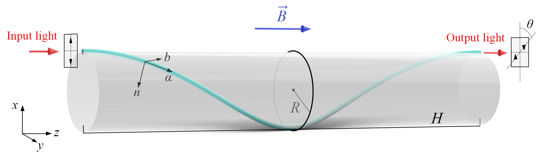
We consider a model of a helically wound nonlinear optical fiber, as illustrated in Fig. 1. A segment of optical fiber with length $L$ is wound around a cylinder of radius $R$, which is placed along the $z$ direction. The pitch of the winding is $H=\sqrt{L^{2}-(2\pi R)^{2}}$. A magnetic field $\vec{B}=\frac{L}{H}B\,\hat{z}$ is applied in the positive $z$ direction, such that the magnetic field intensity in the tangential direction of the optical fiber is equal to $B$. A linearly polarized light beam, polarized along the $x$ direction, is input at the left end of the optical fiber. Due to the presence of the external magnetic field, the helical configuration, and nonlinear effects, the light beam output from the right end will have a polarization direction different from the incident light. The angle by which the polarization direction differs, denoted by $\theta$, is the rotation angle. In the absence of magnetic fields and the nonlinearity, this configuration of light propagation has been considered by Refs. Ross-1984 ; Tomita-1986 ; Berry-1987 .

Influenced by the geometric configuration, the light waves in the wound fiber will always propagate tangentially to the fiber. Studying their propagation in the laboratory coordinate system $(\hat{x},\hat{y},\hat{z})$ is inconvenient. Therefore, we will construct a coordinate system dependent on the geometric configuration—the Frenet coordinate system $(\hat{n},\hat{b},\hat{\alpha})$. The three basis vectors, dependent on the configuration of fiber, have the tangential, normal, and binormal directions of fiber, respectively. When the origins of the two coordinate systems are the same, dependent on the arc length $s$, a position vector $\vec{r}$ can be decomposed in the two coordinate systems as follows:

$\displaystyle\begin{split}\vec{r}=x\,\hat{x}+y\,\hat{y}+z\,\hat{z}=n\,\hat{n}+b\,\hat{b}+\alpha\hat{\alpha},\end{split}$

(1)

thus, this vector can be expressed in both coordinate systems as $\vec{r}_{L}=\begin{bmatrix}x&y&z\end{bmatrix}^{\rm T}$, $\vec{r}_{F}=\begin{bmatrix}n&b&\alpha\end{bmatrix}^{\rm T}$, where subscripts $L$ and $F$ represent representations in the laboratory coordinate system and the Frenet coordinate system, respectively. One can obtain the expressions for the curvature and torsion of the fiber:

$\displaystyle\begin{split}&\kappa=\frac{(2\pi)^{2}R}{L^{2}},\quad\tau=\frac{2\pi H}{L^{2}},\end{split}$

(2)

and the three-dimensional covariant metric tensor:

$\displaystyle\begin{split}g_{ij}=\begin{bmatrix}1&0&G_{1}\\ 0&1&G_{2}\\ G_{1}&G_{2}&G_{1}^{2}+G_{2}^{2}+G_{3}^{2}\\ \end{bmatrix}_{ij},\end{split}$

(3)

where $G_{1}=\kappa\alpha-\tau b,G_{2}=\tau n,G_{3}=1-\kappa n$. The specific calculations about them can be seen in Appendix I.

Before addressing the propagation of polarized lights in the fiber, we need to analyze the nonlinear response of fiber on the light. Considering that the molecules in fiber belong to the symmetric ones, the nonlinear response is mainly described by the third-order susceptibility Agrawal-book . The classical oscillator model can effectively analyze the polarization properties of the medium under non-resonant conditions, where linear and nonlinear polarizations are distinguished by the harmonic and non-harmonic parts of the electron vibration potential Boyd-book . Here, we will utilize the oscillator model to analyze the influence of the external magnetic field on the third-order susceptibility of the optical fiber, preparing for the subsequent calculation of the Faraday rotation angle.

The equation of motion for the electrons in the optical fiber can be expressed as Boyd-book :

$\displaystyle m_{e}\ddot{\vec{r}}=-e\vec{E}-(k_{0}+k_{2}|\vec{r}|^{2})\vec{r}-e\dot{\vec{r}}\times\vec{B},$

(4)

where $e$ and $m_{e}$ are the unit charge quantity and mass of electron. The three terms on the right-hand side represent the electric field force, restoring force, and Lorentz force, respectively. $k_{0}$ and $k_{2}$ are the coefficients of the harmonic and non-harmonic parts of the electron vibration potential. Assuming the electric field vector always lies in the $x$-$y$ plane, at a fixed position, the electric field components can be expressed as:

$\displaystyle E_{j}(t)=\frac{1}{2}(A_{j}e^{-i\omega t}+A_{j}^{*}e^{i\omega t}),$

(5)

where $j=1,2$ corresponding to the directions of $x$ and $y$, respectively. Electrons will always move in the $x$-$y$ plane. Due to the introduction of the non-harmonic potential, the electron’s oscillation will contain two parts: the fundamental part with frequency $\omega$ and the third harmonic part with frequency $3\omega$. Therefore, the displacements in different directions of the electrons can be set as

$\displaystyle r_{j}(t)=\frac{1}{2}[r_{j}^{(1)}e^{-i\omega t}+r_{j}^{(1)*}e^{i\omega t}+r_{j}^{(3)}e^{-3i\omega t}+r_{j}^{(3)*}e^{3i\omega t}],$

(6)

where $r_{1}=x$ and $r_{2}=y$. Considering that the third harmonic part arises from the non-harmonic potential, and the non-harmonic potential is much lower than the harmonic potential, i.e., $k_{2}|\vec{r}|^{2}\ll k_{0}$, we can assume that the amplitude of the third harmonic part is much smaller than that of the fundamental part: $|x^{(3)}|,|y^{(3)}|\ll|x^{(1)}|,|y^{(1)}|$ Boyd-book .

Firstly, substituting Eq. (6) into Eq. (4), retaining terms containing $e^{-i\omega t}$, and ignoring terms containing $k_{2}$ and $x^{(3)},y^{(3)}$, we can solve the amplitudes of the fundamental part $x^{(1)},y^{(1)}$ [see Eq. (A25) in Appendix II], which are the linear functions about $A_{x}$ and $A_{y}$. We know that the linear polarization vector $\vec{P}^{(L)}$ only contains the fundamental wave with frequency $\omega$, and its $i$-th component has two different expressions:

$\displaystyle P^{(L)}_{i}=\epsilon_{0}\chi^{(1)}_{ij}E_{j}=-Ner^{(1)}_{i},$

(7)

where $\chi^{(1)}$ is the first-order susceptibility, and $r^{(1)}_{1}=x^{(1)}$, $r^{(1)}_{2}=y^{(1)}$. From Eq. (7) and the derived expressions of $x^{(1)},y^{(1)}$, we can obtain the matrix form of the first-order susceptibility:

$\displaystyle\chi^{(1)}$

$\displaystyle=\frac{\chi_{0}(\omega)}{1-\Omega_{c}^{2}}\begin{bmatrix}1&i\Omega_{c}\\ -i\Omega_{c}&1\end{bmatrix},$

(8)

where $\Omega_{c}$ is a dimensionless quantity proportional to $B$:

$\displaystyle\Omega_{c}=\frac{\omega\omega_{c}}{\omega_{0}^{2}-\omega^{2}}=\frac{2[1+\chi_{0}(\omega)]}{\chi_{0}(\omega)}\frac{V_{d}B}{\beta},$

(9)

$\omega_{0}=\sqrt{k_{0}/m_{e}}$ is the angular frequency of harmonic vibration, and $\omega_{c}=eB/m_{e}$ is the cyclotron frequency. The Verdet constant is $V_{d}(\omega)=\frac{e\omega}{2m_{e}c}\frac{d{n}}{d\omega}$. $\chi_{0}(\omega)$ is the first-order susceptibility without an external magnetic field:

$\displaystyle\chi_{0}(\omega)=\frac{{Ne^{2}}/{m_{e}\epsilon_{0}}}{\omega_{0}^{2}-\omega^{2}},$

(10)

where $N$ and $\epsilon_{0}$ are the effective density of electron number and permittivity of vacuum. The refractive index without a magnetic field is $n(\omega)=\sqrt{1+\chi_{0}(\omega)}$, and furthermore the propagation constant is $\beta=n(\omega)\omega/c$, where $c$ is the speed of light in vacuum. The tensor $\chi^{(1)}$ in Eq. (8) possesses rotational invariance,

$\displaystyle\chi^{(1)}_{i^{\prime}j^{\prime}}={\rm R}^{-1}_{i^{\prime}i}\chi^{(1)}_{ij}{\rm R}_{jj^{\prime}},\quad{\rm R}_{ij}=\begin{bmatrix}\cos\theta&\sin\theta\\ -\sin\theta&\cos\theta\end{bmatrix}_{ij},$

(11)

which is an important property ensuring that the third-order susceptibility remains unchanged during the rotation of the optical fiber. Therefore, the effects of slight twisting during the coiling process can be ignored. In current experiments of optical fiber, we always have $V_{d}B\ll\beta$, so we neglect the second-order term of $\Omega_{c}$ and obtain $\chi^{(1)}=\chi_{0}(\mathbf{I}-\Omega_{c}\hat{\sigma}_{2})$, where $\hat{\sigma}_{2}$ is Pauli matrix.

Next, substituting equation (6) into equation (4), retaining terms containing $e^{-3i\omega t}$, and ignoring higher-order terms of $k_{2}$ and $x^{(3)},y^{(3)}$, we obtain the amplitudes of the third-harmonic part $x^{(3)},y^{(3)}$ [see Eq. (A28) in Appendix II], which are the nonlinear functions about $A_{x}$ and $A_{y}$. We know that the nonlinear polarization vector has the following form:

	$\displaystyle{P}_{i}^{(N)}$	$\displaystyle=\epsilon_{0}{\chi}^{(3)}_{ijkl}E_{j}E_{k}E_{l}$
		$\displaystyle=\frac{\epsilon_{0}}{8}{\chi}^{(3)}_{ijkl}[({A^{*}_{j}}A_{k}A_{l}+A_{j}{A^{*}_{k}}A_{l}+A_{j}A_{k}{A^{*}_{l}})e^{-i\omega t}$
		$\displaystyle\qquad+({A_{j}}A^{*}_{k}A^{*}_{l}+A^{*}_{j}{A_{k}}A^{*}_{l}+A^{*}_{j}A^{*}_{k}{A_{l}})e^{i\omega t}$
		$\displaystyle\qquad+A_{j}A_{k}A_{l}e^{-3i\omega t}+A_{j}^{*}A_{k}^{*}A_{l}^{*}e^{3i\omega t}]$
		$\displaystyle\equiv\frac{1}{2}(N_{i}^{(1)}e^{-i\omega t}+N_{i}^{(1)*}e^{i\omega t}+N_{i}^{(3)}e^{-3i\omega t}+N_{i}^{(3)*}e^{3i\omega t}),$		(12)

where $N_{i}^{(1)}$ and $N_{i}^{(3)}$ are the amplitudes of the fundamental and the third harmonic parts, respectively. For the third harmonic part, there is a relationship between the nonlinear polarization vector and the electron displacement vector (their $i$-th components are $P_{i}^{(N)}$ and $r_{i}$, respectively): $P_{i}^{(N)}|_{3\omega}=-Ner_{i}|_{3\omega}$. Here $N$ is the number of electrons per unit volume. From Eqs. (II.2) and (6), we know $N_{x}^{(3)}=-Nex^{(3)}$ and $N_{y}^{(3)}=-Ney^{(3)}$. By comparing them with equation (II.2), we can obtain the components of the third-order susceptibility tensor $\chi^{(3)}$:

		$\displaystyle\chi^{(3)}_{xxxx}=\chi^{(3)}_{yyyy}=-\frac{\epsilon_{0}^{3}\chi_{0}^{3}(\omega)\chi_{0}(3\omega)}{N^{3}e^{4}}k_{2},$		(13a)
		$\displaystyle\chi^{(3)}_{xxyy}=\chi^{(3)}_{xyyx}=\chi^{(3)}_{xyxy}=\chi^{(3)}_{yxxy}=\chi^{(3)}_{yyxx}=\chi^{(3)}_{yxyx}=\frac{1}{3}\chi^{(3)}_{xxxx},$		(13b)
		$\displaystyle\chi^{(3)}_{xyyy}=-\chi^{(3)}_{yxxx}=\frac{4i\chi_{0}(3\omega)}{\chi_{0}(\sqrt{3}\omega)}\Omega_{c}\chi^{(3)}_{xxxx},$		(13c)
		$\displaystyle\chi^{(3)}_{xxxy}=\chi^{(3)}_{xxyx}=\chi^{(3)}_{xyxx}=\frac{1}{3}\chi^{(3)}_{xyyy},$		(13d)
		$\displaystyle\chi^{(3)}_{yxyy}=\chi^{(3)}_{yyxy}=\chi^{(3)}_{yyyx}=-\frac{1}{3}\chi^{(3)}_{xyyy}.$		(13e)

This tensor $\chi^{(3)}$ also possesses rotational invariance, $\chi^{(3)}_{i^{\prime}j^{\prime}k^{\prime}l^{\prime}}={\rm R}^{-1}_{i^{\prime}i}{\rm R}^{-1}_{j^{\prime}j}\chi^{(3)}_{ijkl}{\rm R}_{kk^{\prime}}{\rm R}_{ll^{\prime}}$, to ensure that it remains unchanged during the rotation of the optical fiber in tangential direction. In the absence of the external magnetic field ($\Omega_{c}=0$), the last eight elements of this tensor will become $0$, and the derived $\chi^{(3)}$ is the same as the result in Ref. Boyd-book .

We consider a helically wound single-mode nonlinear fiber, as shown in Fig. 1. Due to the polarization vector $\vec{P}=\vec{P}^{(L)}+\vec{P}^{(N)}$, in the Frenet coordinate system, the propagation equation of electric field of the light is

$\displaystyle\frac{\partial^{2}\vec{E}(s,t)}{\partial s^{2}}=\frac{1}{c^{2}}\frac{\partial^{2}\vec{E}(s,t)}{\partial t^{2}}+\mu_{0}\frac{\partial^{2}\vec{P}^{(L)}(s,t)}{\partial t^{2}}+\mu_{0}\frac{\partial^{2}\vec{P}^{(N)}(s,t)}{\partial t^{2}},$

(14)

where the electric field vector $\vec{E}(s,t)=E_{n}(s,t)\hat{n}(s)+E_{b}(s,t)\hat{b}(s)$, and the propagation distance is represented by the arc length $s$. The specific calculation process of Eq. (14) can be seen in Appendix I. When we input a continuous wave, the electric field vector can be written as

$\displaystyle\begin{split}\vec{E}(s,t)=\frac{1}{2}[\vec{A}(s)\,e^{i({\beta}s-\omega t)}+\vec{A}^{*}(s)\,e^{-i({\beta}s-\omega t)}],\end{split}$

(15)

where the propagation constant is $\beta=n(\omega)\omega/c$ and the complex amplitude vector of the electric field is $\vec{A}(s)=A_{n}(s)\hat{n}(s)+A_{b}(s)\hat{b}(s)$.

The linear polarization vector is $\vec{P}^{(L)}(s,t)=\epsilon_{0}\chi^{(1)}\vec{E}(s,t)$, where the first-order susceptibility has the expression (8); the nonlinear one is $\vec{P}^{(N)}(s,t)=\epsilon_{0}{\chi}^{(3)}\vdots\,\vec{E}(s,t)\vec{E}(s,t)\vec{E}(s,t)$, where the third-order susceptibility has the expression (13a). Ignoring the third-harmonic waves in the fiber, we recall the nonlinear polarization vector (II.2) and write

$\displaystyle\vec{P}^{(N)}(s)=\frac{1}{2}[\vec{N}^{(1)}(s)e^{i({\beta}s-\omega t)}+\vec{N}^{*(1)}(s)e^{-i({\beta}s-\omega t)}].$

(16)

where $\vec{N}^{(1)}(s)=N_{n}^{(1)}(s)\hat{n}(s)+N_{b}^{(1)}(s)\hat{b}(s)$ and

$\displaystyle\begin{split}{N}_{i}^{(1)}=\frac{\epsilon_{0}}{4}{\chi}^{(3)}_{ijkl}({A^{*}_{j}}A_{k}A_{l}+A_{j}{A^{*}_{k}}A_{l}+A_{j}A_{k}{A^{*}_{l}}).\end{split}$

(17)

Furthermore, substituting the expression (13a) of $\chi^{(3)}$ into it, one can obtain

	$\displaystyle N_{n}^{(1)}=\frac{3\epsilon_{0}}{4}{\chi}^{(3)}_{xxxx}\Big{(}h_{1}+iC_{B}\frac{V_{d}B}{\beta}h_{2}\Big{)},$		(18a)
	$\displaystyle N_{b}^{(1)}=\frac{3\epsilon_{0}}{4}{\chi}^{(3)}_{xxxx}\Big{(}h_{2}-iC_{B}\frac{V_{d}B}{\beta}h_{1}\Big{)}.$		(18b)

where

	$\displaystyle h_{1}=(|{A_{n}}|^{2}+\frac{2}{3}|{A_{b}}|^{2})A_{n}+\frac{1}{3}{A^{*}_{n}}A_{b}^{2},$		(19a)
	$\displaystyle h_{2}=(\frac{2}{3}|{A_{n}}|^{2}+|{A_{b}}|^{2})A_{b}+\frac{1}{3}A_{n}^{2}{A^{*}_{b}},$		(19b)

and $C_{B}$ is a dimensionless function about light frequency:

$\displaystyle C_{B}=\frac{8\chi_{0}(3\omega)[1+\chi_{0}(\omega)]}{\chi_{0}(\omega)\chi_{0}(\sqrt{3}\omega)}.$

(20)

Next, we substitute the expressions of $\vec{E}$ (15), $\vec{P}^{(L)}$, and $\vec{P}^{(N)}$ (16) into Eq. (14) to obtain:

$\displaystyle 2i\beta\frac{d\vec{A}}{ds}+\frac{d^{2}\vec{A}}{ds^{2}}-2\beta V_{d}B\hat{\sigma}_{2}\vec{A}+\mu_{0}\omega^{2}\vec{N}^{(1)}=0.$

(21)

Due to $\frac{d\hat{\alpha}}{ds}=\kappa\hat{n}$, $\frac{d\hat{n}}{ds}=-\kappa\hat{\alpha}+\tau\hat{b}$, $\frac{d\hat{b}}{ds}=-\tau\hat{n}$, considering the slowly varying envelope approximation and neglecting the terms of $\frac{d^{2}A_{i}}{ds^{2}}$ in the above equations, we can obtain

	$\displaystyle\frac{dA_{n}}{ds}=\frac{i\beta(\tau^{2}-\kappa^{2}-2V_{d}B\tau)}{2(\beta^{2}-\tau^{2})}A_{n}+\frac{2\beta^{2}\tau-\tau^{3}-2V_{d}B\beta^{2}}{2(\beta^{2}-\tau^{2})}A_{b}$
	$\displaystyle\qquad+\frac{i\mu_{0}\omega^{2}}{2(\beta^{2}-\tau^{2})}(\beta N_{n}-i\tau N_{b}),$		(22a)
	$\displaystyle\frac{dA_{b}}{ds}=\frac{\tau(\kappa^{2}+\tau^{2}-2\beta^{2})+2V_{d}B\beta^{2}}{2(\beta^{2}-\tau^{2})}A_{n}+\frac{i\beta\tau(\tau-2V_{d}B)}{2(\beta^{2}-\tau^{2})}A_{b}$
	$\displaystyle\qquad+\frac{i\mu_{0}\omega^{2}}{2(\beta^{2}-\tau^{2})}(i\tau N_{n}+\beta N_{b}).$		(22b)

Then, we consider the practical condition $\tau,\kappa,V_{d}B\ll\beta$, neglect the quadratic terms of the small quantities $\tau/\beta$, $\kappa/\beta$, and $V_{d}B/\beta$, and substitute the expressions (18) of $N_{n}$ and $N_{b}$ into the above equations. Due to practical reasons, in Eq. (18), $A_{x}$ and $A_{y}$ are expressed in units of electric field (V/m). We introduce $\vec{A}^{\prime}$ such that $|\vec{A}^{\prime}|^{2}$ to represent optical power:

$\displaystyle|\vec{A}^{\prime}|^{2}=\frac{1}{2}nc\epsilon_{0}S|\vec{A}|^{2},$

(23)

where $S$ is the effective cross-sectional area of the fiber core. After substituting the above relation, for simplicity, we omit the prime notation from $A^{\prime}_{x}$ and $A^{\prime}_{y}$. Then we can obtain:

	$\displaystyle i\frac{d\vec{A}}{ds}=\Big{[}\hat{K}+(V_{d}B-\tau)\hat{\sigma}_{2}$	$\displaystyle+\frac{1}{\beta}(\tau+C_{B}V_{d}B)\hat{\sigma}_{2}\hat{h}^{\prime}$
		$\displaystyle+(1+\frac{V_{d}B\tau}{\beta^{2}}C_{B})\hat{h}^{\prime}\Big{]}\vec{A},$		(24)

where $\hat{h}^{\prime}$ is the Homitonian in a straight nonlinear fiber when the magnetic field is absent:

$\displaystyle\hat{h}^{\prime}=-\sigma^{\prime}\begin{bmatrix}|{A_{n}}|^{2}+\frac{2}{3}|{A_{b}}|^{2}&\frac{1}{3}A_{n}^{*}A_{b}\\ \frac{1}{3}A_{n}A_{b}^{*}&\frac{2}{3}|{A_{n}}|^{2}+|{A_{b}}|^{2}\\ \end{bmatrix},$

(25)

and $\sigma^{\prime}=\frac{3{\chi}^{(3)}_{xxxx}\omega}{4n^{2}c^{2}\epsilon_{0}S}$. The matrix $\hat{K}$ is

$\displaystyle\hat{K}=\begin{bmatrix}\frac{\kappa^{2}}{2\beta}&0\\ 0&0\\ \end{bmatrix}+\frac{2V_{d}B\tau-\tau^{2}}{2\beta}\begin{bmatrix}1&0\\ 0&1\end{bmatrix}.$

(26)

The first part arises from the linear birefringence induced by curvature $\kappa$, which can be neglected by considering $2\pi R\ll H$ such that $\kappa\ll\tau$. The second part represents the change in propagation constants, but due to $\Delta\beta=\frac{2V_{d}B\tau-\tau^{2}}{2\beta}\ll\beta$, it can be ignored. Therefore, we can ignore $\hat{K}$ and the quadratic small quantity $\frac{V_{d}B\tau}{\beta^{2}}$, yielding:

$\displaystyle i\frac{d\vec{A}}{ds}=\Big{[}(V_{d}B-\tau)\hat{\sigma}_{2}+\frac{1}{\beta}(\tau+C_{B}V_{d}B)\hat{\sigma}_{2}\hat{h}^{\prime}+\hat{h}^{\prime}\Big{]}\vec{A}.$

(27)

This is the evolution equation of the amplitude vector $\vec{A}$ with the arc length $s$.

Three interesting situations will be discussed as follows. In the absence of the nonlinear effect ($\sigma^{\prime}=0$), Eq. (27) will become $i\partial_{s}\vec{A}=(V_{d}B-\tau)\hat{\sigma}_{2}\vec{A}$, where the equivalence between $V_{d}B$ and $\tau$ indicates that the torsion $\tau$ can be viewed as an effective magnetic field Berry-1987 ; Ross-1984 ; Tabor-1969 ; Smith-1978 ; Rashleigh-1983 , i.e., the so-called geometry-induced gauge fields Guinea-2010 ; Zhang-2014 ; Wang-2014 ; Tan-2021 ; Wang-2022 . In a straight fiber without the external magnetic field ($B=0$ and $\tau=0$), Eq. (27) will become $i\partial_{s}\vec{A}=\hat{h}^{\prime}\vec{A}$, which describes the evolution of a continuous wave in an isotropic nonlinear fiber Crosignani-1985 ; Trillo-1986 ; Akhmediev-1994 ; Barad-1997 . In a helically wound fiber with an external magnetic field, Eq. (27) describes the evolution of a continuous wave under the combined impact of the magnetic field, helical geometry, and the nonlinear effect. In this equation, the term $\frac{1}{\beta}(\tau+C_{B}V_{d}B)\hat{\sigma}_{2}\hat{h}^{\prime}$ manifests an interesting interplay between the three effects, providing a comparable correction of rotation angle in the cases with intense lights.

We analyze the evolution of polarization states in this system from another perspective Barad-1997 . Introducing the Stokes vector $\vec{S}=S_{x}\hat{e}_{x}+S_{y}\hat{e}_{y}+S_{z}\hat{e}_{z}$, where the components are defined as:

$\displaystyle S_{x}=|A_{x}|^{2}-|A_{y}|^{2},\;S_{y}=A_{x}^{*}A_{y}+A_{x}A_{y}^{*},\;S_{z}=i(A_{x}A_{y}^{*}-A_{x}^{*}A_{y}).$

(28)

It’s noted that the amplitude of this vector is conserved: $|\vec{S}|=|A_{x}|^{2}+|A_{y}|^{2}=A^{2}$, i.e., it equals to the light power. Substituting Eq. (28) into Eq. (27), we obtain:

$\displaystyle\frac{d\vec{S}}{dz}=-2\Big{[}V_{d}B-\tau-\frac{\sigma^{\prime}A^{2}}{\beta}(\tau+C_{B}V_{d}B)+\frac{1}{3}{\sigma^{\prime}}S_{z}\Big{]}\vec{S}\times\hat{e}_{z}.$

(29)

It describes the rotation of vector $\vec{S}$ around $\hat{e}_{z}$ axis, which indicates that $S_{z}$ is conserved. The rotation solution to this motion equation is:

$\displaystyle\vec{S}$

$\displaystyle=(S_{x},S_{y},S_{z})=A^{2}\cos 2\chi[\cos(2\Omega z),\,\sin(2\Omega z),\,\tan 2\chi],$

(30)

where

$\displaystyle\Omega=V_{d}B-\tau-\frac{\sigma^{\prime}A^{2}}{\beta}(\tau+C_{B}V_{d}B)+\frac{1}{3}{\sigma^{\prime}}A^{2}\sin 2\chi.$

(31)

$\chi$ represents the elliptic angle, whose zero or non-zero values correspond to linearly or elliptically polarized states, respectively.

The solution (30) describes a rotation process of different polarized states in the Poincar$\rm\acute{e}$ sphere. Its rotation frequency of $\vec{S}$ in the sphere is twice the rotation frequency of the light’s polarization in the real space of $n$-$b$. Therefore, we can derive the rotation angle per unit length for linearly polarized light ($\chi=0$) as:

$\displaystyle{\theta}/{l}=\Omega=\Big{(}1-C_{B}\frac{\sigma^{\prime}A^{2}}{\beta}\Big{)}V_{d}B-\Big{(}1+\frac{\sigma^{\prime}A^{2}}{\beta}\Big{)}\tau,$

(32)

and for elliptically polarized light ($\chi\neq 0$) as:

$\displaystyle{\theta}/{l}=\Omega=\Big{(}1-$

$\displaystyle C_{B}\frac{\sigma^{\prime}A^{2}}{\beta}\Big{)}V_{d}B-\Big{(}1+\frac{\sigma^{\prime}A^{2}}{\beta}\Big{)}\tau+\frac{1}{3}{\sigma^{\prime}}A^{2}\sin 2\chi,$

(33)

where $\theta$ is total rotation angle of light and $l$ is total propagation distance,. The dimensionless quantity $C_{B}$ has the expression (20), which measures the impact of nonlinear effect on the Faraday rotation angle. For a nonlinear fiber, the rotation angle $\theta/l$ in different situations is illustrated in Tab. 1.

We firstly focus on the rotation of linearly polarized light, as shown in the second row of Tab. 1. In a straight fiber with an external magnetic field, nonlinear effects will exert a correction on the Verdet constant, resulting in a modified Verdet constant of $V_{d}^{(N)}=(1-C_{B}\frac{\sigma^{\prime}A^{2}}{\beta})V_{d}$. Similarly, in a helically wound fiber without an external magnetic field, nonlinear effects will also influence the rotation angle in the Faraday-like effect, equivalent to exerting a correction to the torsion of the fiber, resulting in a modified torsion of $\tau^{(N)}=(1+\frac{\sigma^{\prime}A^{2}}{\beta})\tau$. When considering both the winding of the fiber and the external magnetic field simultaneously, the obtained rotation angle is a linear combination of the first two results.

Then, we shift our focus to elliptically polarized light, as shown in the third row of Tab. 1. In the three cases mentioned above, the only difference between the rotation angles of linearly and elliptically polarized light is the emergence of an additional term $\frac{1}{3}{\sigma^{\prime}}A^{2}\sin 2\chi$. It indicates that the rotation angle of an elliptically polarized light will also depend on its own ellipticity angle $\chi$. In a straight fiber without an external magnetic field, due to the presence of this term, an elliptically polarized light also exhibits rotation. This kind of intensity-induced rotation is fundamentally different from the Faraday and Faraday-like rotations, and has been earlier studied in various systems including nonlinear fibers Crosignani-1985 ; Maker-1964 ; Agrawal-book .

Among these situations in Tab. 1, an interesting one is a helically wound optical fiber without an external magnetic field, where the rotation angle is $\theta/l=-(1+\frac{\sigma^{\prime}A^{2}}{\beta})\tau$. In the absence of the nonlinearity, the torsion geometry serves as the magnetic field, and is closely related to the celebrated Berry phase, as discussed by Ref. Berry-1987 . The geometry induced gauge field is rather interesting and constantly attract much attention Wang-2014 ; Wang-2022 . In the presence of the nonlinearity, it is seen that the rotation angle is due to the interplay between the geometry and nonlinearity, which indicates the emergence of a nonlinear Berry phase Liu-2010 ; Liu-book .

Parameter Settings We use the optical fibers made of $\rm As_{2}S_{3}$ as the medium for light propagation, which is a type of chalcogenide fiber. Compared to traditional $\rm SiO_{2}$ fibers, this type of fiber exhibits larger nonlinear refractive index and Verdet constant, making it suitable for observing nonlinear and magnetic field-induced effects. The nonlinear refractive index Sanghera-2008 and the Verdet constant Ruan-2005 of $\rm As_{2}S_{3}$ fibers have been measured in previous experiments, and here we will refer to the parameters provided in the two experimental works.

Firstly, for the nonlinearity coefficient $k_{2}$, we can estimate it using the following formula Boyd-book :

$\displaystyle k_{2}=-\frac{k_{0}}{d^{2}}=-\frac{m_{e}\omega_{0}^{2}}{d^{2}},$

(34)

where $\omega_{0}$ is the lowest resonant frequency of the atom. $d$ is a typical value for the atomic scale, which can be taken as the Bohr radius: $d\approx a_{0}=\frac{4\pi\epsilon_{0}\hbar^{2}}{m_{e}e^{2}}$.

In the non-resonant limit ($\omega\ll\omega_{0}$), from Eq. (10), the first-order polarization without an external magnetic field can be expressed as:

$\displaystyle\chi_{0}\approx\frac{Ne^{2}}{m_{e}\epsilon_{0}\omega_{0}^{2}}.$

(35)

Meanwhile, from Eq. (13a), the typical component of the third-order polarization can be written as:

$\displaystyle\chi_{xxxx}$

$\displaystyle=-\frac{\epsilon_{0}^{3}\chi_{0}^{3}(\omega)\chi_{0}(3\omega)}{N^{3}e^{4}}k_{2}\approx\frac{Ne^{4}}{m_{e}^{3}\epsilon_{0}d^{2}\omega_{0}^{6}}.$

(36)

The Verdet constant can be written as:

	$\displaystyle V_{d}=\frac{e\omega}{2m_{e}c}\frac{d{n}}{d\omega}$	$\displaystyle=\frac{N\epsilon_{0}e^{3}\omega^{2}}{2c\sqrt{\epsilon_{0}m_{e}(\omega_{0}^{2}-\omega^{2})+Ne^{2}}}$
		$\displaystyle\approx\frac{N\epsilon_{0}e^{3}\omega^{2}}{2c\sqrt{\epsilon_{0}m_{e}\omega_{0}^{2}+Ne^{2}}}$		(37)

It has been experimentally measured that the lowest bandgap of $\rm As_{2}S_{3}$ is $E_{g}=2.38\,{\rm eV}$, thus the lowest resonant frequency is $\omega_{0}=E_{g}/\hbar=3.6\times 10^{15}\,{\rm Hz}$. Based on it, the following are the calculations of some parameters:

• •

  Density of $\rm As_{2}S_{3}$ fiber: $\rho=3.46\,{\rm g/cm^{3}}$, molecular mass: $M=246.04\times 1.661\times 10^{-27}\,{\rm kg}$, thus the number density of molecules: $N=\rho/M=8.47\times 10^{27}/{\rm m^{3}}$.

• •

  Refractive index: $n=\sqrt{1+\chi_{0}}=1.75$, experimental result: $\bar{n}=2.4$.

• •

  Typical component of the third-order polarization: $\chi_{xxxx}=1.33\times 10^{-19}\,{\rm m^{2}/V^{2}}$, experimental result: $\bar{\chi}_{xxxx}=4.1\times 10^{-19}\,{\rm m^{2}/V^{2}}$.

• •

  Nonlinear refractive index: $n_{2}=\frac{3}{4n^{2}\epsilon_{0}c}\chi^{(3)}_{xxxx}=1.23\times 10^{-17}\,{\rm m^{2}/W}$, experimental result: $\bar{n}_{2}=2\times 10^{-17}\,{\rm m^{2}/W}$.

• •

  Verdet constant: $V_{d}=39.2\,{\rm/T/m}$, experimental result: $\bar{V}_{d}=14.5{\rm/T/m}$.

Nonlinear Correction to Verdet Constant Here, we focus on the situation of a straight fiber to discuss the correction induced by the third-order nonlinear effect for Verdet constant. From Eqs. (32) and (33), in the presence of an external magnetic field and considering third-order nonlinear effects, the rotation angle per unit distance of linearly polarized light ($\chi=0$) in a straight fiber is given by

$\displaystyle\theta/l=\Omega=\Big{(}1-\frac{\sigma^{\prime}A^{2}}{\beta}C_{B}\Big{)}V_{d}B,$

(38)

and the one of elliptically polarized light ($\chi\neq 0$) is given by

$\displaystyle\theta/l=\Omega=\Big{(}1-\frac{\sigma^{\prime}A^{2}}{\beta}C_{B}\Big{)}V_{d}B+\frac{1}{3}{\sigma^{\prime}}A^{2}\sin 2\chi.$

(39)

$C_{B}$ is an important parameter, measuring the influence of third-order nonlinear effects on the Faraday rotation angle. Interestingly, it can considered as a nonlinear correction to the Verdet constant, i.e., in the nonlinear case, the Verdet constant becomes

$\displaystyle V_{d}^{(N)}=\Big{(}1-\frac{\sigma^{\prime}A^{2}}{\beta}C_{B}\Big{)}V_{d}.$

(40)

In the non-resonant limit, from Eq. (20), the parameter $C_{B}$ can be approximated as:

$\displaystyle C_{B}\approx\frac{8(1+\chi_{0})}{\chi_{0}}=\frac{8n^{2}}{n^{2}-1}=8\Big{(}1+\frac{m_{e}\epsilon_{0}\omega_{0}^{2}}{Ne^{2}}\Big{)}.$

(41)

Using the practical refractive index $\bar{n}$, the value of $C_{B}$ in $\rm As_{2}S_{3}$ fibers is $C_{B}=8\bar{n}^{2}/(\bar{n}^{2}-1)=11.33$. In materials with refractive index greater than 1, the value of $C_{B}$ decreases with increasing refractive index.

According to Ref. Sanghera-2008 , we take the diameter of the fiber core as $d_{c}=4.2\,{\rm\mu m}$, core cross-sectional area as $S=13.85\,{\rm\mu m^{2}}$, incident wavelength as $\lambda=1550\,{\rm nm}$, and propagation constant as $\beta=2\pi/\lambda=5.87\times 10^{6}\,{\rm m^{-1}}$. Assuming the light has approximately uniform distribution in the radial direction, we can obtain the nonlinear coefficient $\sigma^{\prime}$ as

$\displaystyle\sigma^{\prime}=\frac{2\pi\bar{n}_{2}}{\lambda S}=5.85\,{\rm/W/m}=3.6\,{\rm/W/m}.$

(42)

For a linearly polarized light, according to Eq. (32), we need $C_{B}\sigma^{\prime}A^{2}/\beta$ to be comparable to 1 to ensure the correction part is significant. Here, we set the condition as $C_{B}\sigma^{\prime}A^{2}/\beta>0.01$, which results in a required optical power: $A^{2}>0.01\beta/\sigma^{\prime}C_{B}=611.6\,{\rm W}$, thus the required incident intensity is $I=A^{2}/S>4.42\times 10^{9}\,{\rm W/cm^{2}}$.

References

- (1) M. Faraday, II. Experimental researches in electricity. Twentieth series, Philos. Trans. R. Soc. London 136, 1 (1846).
- (2) L. J. Aplet and J. W. Carson, A Faraday effect optical isolator, Applied Optics 3, 544 (1964).
- (3) H. Takeda and S. John, Compact optical one-way waveguide isolators for photonic-band-gap microchips, Phys. Rev. A 78, 023804 (2008).
- (4) D. K. Efimkin and Yu. E. Lozovik, Resonant manifestations of chiral excitons in Faraday and Kerr effects in a topological insulator film, Phys. Rev. B 87, 245416 (2013).
- (5) P. Mihailovic and S. Petricevic, Fiber optic sensors based on the Faraday effect, Sensors 21, 6564 (2021).
- (6) D. Budker, D. F. Kimball, S. M. Rochester, V. V. Yashchuk, and M. Zolotorev, Sensitive magnetometry based on nonlinear magneto-optical rotation, Phys. Rev. A 62, 043403 (2000).
- (7) R. W. Boyd, Nonlinear Optics (Academic Press, Elsevier, 2008).
- (8) K. Sato and T. Ishibashi, Fundamentals of magneto-optical spectroscopy, Front. Phys.-Lausanne 10, 946515 (2022).
- (9) H. S. Bennett and E. A. Stern, Faraday effect in solids, Phys. Rev. 137, A448 (1965).
- (10) P. N. Schatz and A. J. McCaffery, The faraday effect, Q. Rev. Chem. Soc. 23, 552 (1969).
- (11) S. I. Kanorsky, A. Weis, J. Wurster, and T. W. Hansch, Quantitative investigation of the resonant nonlinear Faraday effect under conditions of optical hyperfine pumping, Phys. Rev. A 47, 1220 (1993).
- (12) D. Budker, W. Gawlik, D. F. Kimball, S. M. Rochester, V. V. Yashchuk, and A. Weis, Resonant nonlinear magneto-optical effects in atoms, Rev. Mod. Phys. 74, 1153 (2002).
- (13) C. Zhu, L. Deng, and E. W. Hagley, Linear and nonlinear Faraday rotations of light polarization in a four-level active-Raman-gain medium, Phys. Rev. A 88, 023854 (2013).
- (14) J. N. Ross, The rotation of the polarization in low birefringence monomode optical fibres due to geometric effects, Opt. Quant. Electron. 16, 455 (1984).
- (15) A. Tomita and R. Y. Chiao, Observation of Berry’s topological phase by use of an optical fiber, Phys. Rev. Lett. 57, 937 (1986).
- (16) M. V. Berry, Quantal phase factors accompanying adiabatic changes, Proc. R. Soc. Lond. A 392, 45 (1984).
- (17) R. Y. Chiao and Y. S. Wu, Manifestations of Berry’s topological phase for the photon, Phys. Rev. Lett. 57, 933 (1986).
- (18) M. V. Berry, Interpreting the anholonomy of coiled light, Nature 326, 277 (1987).
- (19) M. Kugler and S. Shtrikman, Berry’s phase, locally inertial frames, and classical analogues, Phys. Rev. D 37, 934 (1988).
- (20) C. Cisowski, J. B. Götte, and S. Franke-Arnold, Colloquium: Geometric phases of light: Insights from fiber bundle theory, Rev. Mod. Phys. 94, 031001 (2022).
- (21) T. Brabec and F. Krausz, Intense few-cycle laser fields: Frontiers of nonlinear optics, Rev. Mod. Phys. 72, 545 (2000).
- (22) J. Toulouse, Optical nonlinearities in fibers: review, recent examples, and systems applications, J. Lightwave Technol. 23, 3625 (2005).
- (23) Y. J. Yu and R. K. Osborn, Effect of a nonlinear refractive index on Faraday rotation, Phys. Rev. A 15, 2404 (1977).
- (24) S. Giraud-Cotton, V. P. Kaftandjian, and L. Klein L, Magnetic optical activity in intense laser fields. I. Self-rotation and Verdet constant, Phys. Rev. A 32, 2211 (1985).
- (25) G. Keiser, Optical Fiber Communications (Wiley, New York, 2003).
- (26) G. W. Day, D. N. Payne, A. J. Barlow, and J. J. Ramskov-Hansent, Faraday rotation in coiled, monomode optical fibers: isolators, filters, and magnetic sensors, Opt. Lett. 7, 238 (1982).
- (27) V. Annovazzi-Lodi, S. Donati, and S. Merlo, Coiled-fiber sensor for vectorial measurement of magnetic field, J. Lightwave Technol. 10, 2006 (1992).
- (28) B. Lee, Review of the present status of optical fiber sensors, Opt. Fiber Technol. 9, 57 (2003).
- (29) J. Liu and L. B. Fu, Berry phase in nonlinear systems, Phys. Rev. A 81, 052112 (2010).
- (30) J. Liu, S. -C. Li, L. -B. Fu, and D. -F. Ye, Nonlinear Adiabatic Evolution of Quantum Systems: Geometric Phase and Virtual Magnetic Monopole. Springer, 2018, 49-72.
- (31) L. D. Zhang, L.B. Fu, and J. Liu, Adiabatic geometric phase in the nonlinear coherent coupler, Eur. Phys. J. D 65, 557–561 (2011).
- (32) W. J. Tabor and F. S. Chen, Electromagnetic Propagation through Materials Possessing Both Faraday Rotation and Birefringence: Experiments with Ytterbium Orthoferrite, J. Appl. Phys. 40, 2760 (1969).
- (33) A. M. Smith, Polarization and magnetooptic properties of single-mode optical fiber, Appl. Opt. 17, 52 (1978).
- (34) S. Rashleigh, Origins and control of polarization effects in single-mode fibers, J. Lightwave Technol. 1, 312 (1983).
- (35) F. Guinea, M. I. Katsnelson, and A. K. Geim, Energy gaps and a zero-field quantum Hall effect in graphene by strain engineering, Nat. Phys. 6, 30 (2010).
- (36) D. -B. Zhang, G. Seifert, and K. Chang,Strain-induced pseudomagnetic fields in twisted graphene nanoribbons, Phys. Rev. Lett. 112, 096805 (2014).
- (37) Y. L. Wang, L. Du, C. T. Xu, X. J. Liu, and H. S. Zong, Pauli equation for a charged spin particle on a curved surface in an electric and magnetic field, Phys. Rev. A 90, 042117 (2014).
- (38) X. Tan, D.-W. Zhang, W. Zheng, X. Yang, S. Song, Z. Han, Y. Dong, Z. Wang, D. Lan, H. Yan, S.-L. Zhu, and Y. Yu, Experimental observation of tensor monopoles with a superconducting qudit, Phys. Rev. Lett. 126, 017702 (2021).
- (39) Y. L. Wang, H. Zhao, H. Jiang, H. Liu, and Y. F. Chen, Geometry-induced monopole magnetic field and quantum spin Hall effects, Phys. Rev. B 106, 235403 (2022).
- (40) B. Crosignani and P. Di Porto, Intensity-induced rotation of the polarization ellipse in low-birefringence, single-mode optical fibres, Optica Acta: Int. J. Opt. 32, 1251 (1985).
- (41) S. Trillo, S. Wabnitz, R. H. Stolen, G. Assanto, C. T. Seaton, and G. I. Stegeman, Experimental observation of polarization instability in a birefringent optical fiber, Appl. Phys. Lett. 49, 1224 (1986).
- (42) N. Akhmediev, A. Buryak, and J. M. Soto-Crespo, Elliptically polarised solitons in birefringent optical fibers, Opt. Commun. 112, 278 (1994).
- (43) Y. Barad and Y. Silberberg, Polarization evolution and polarization instability of solitons in a birefringent optical fiber, Phys. Rev. Lett. 78, 3290 (1997).
- (44) G. P. Agrawal, Nonlinear fiber optics, (Academic, 2007)
- (45) P. D. Maker, R. W. Terhune, and C. M. Savage, Intensity-dependent changes in the refractive index of liquids, Phys. Rev. Lett. 12, 507 (1964).
- (46) J. S. Sanghera, C. M. Florea, L. B. Shaw, P. Pureza, V. Q. Nguyen, M. Bashkansky, Z. Dutton, and I. D. Aggarwal, Non-linear properties of chalcogenide glasses and fibers, J. Non-Cryst. Solids 354, 462 (2008).
- (47) Y. Ruan, R. A. Jarvis, A. V. Rode, S. Madden, and B. Luther-Davies, Wavelength dispersion of Verdet constants in chalcogenide glasses for magneto-optical waveguide devices, Opt. Commun. 252, 39 (2005).