Nonlinear dynamics of oscillons and transients during preheating after single field inflation
Abstract
In the single-field model, the preheating process occurs through self-resonance of inflaton field. We study the nonlinear structures generated during preheating in the -attractor models and monodromy models. The potentials have a power law form near the origin and a flat region away from bottom, which are consistent with current cosmological observations. The Floquet analysis shows that potential parameters in monodromy model have a significant influence on the region of resonance bands. The analytical oscillons solution for the -attractor T model with parameter is derived using the small amplitude analysis method. Besides we investigate the formation of nonlinear structures, the equation of state and the energy transfer through the (3+1) dimensional lattice simulation. We find that the symmetric T potential and the asymmetric E potential in the -attractor models have similar nonlinear dynamics. And the potential parameter in monodromy model significantly influences the lifetime of transients, whereas the parameter exerts minimal impact on the nonlinear dynamics.
I Introduction
The single field inflation driven by a power-law potential is ruled out by the measurements of cosmic microwave background (CMB) anisotropies Aghanim et al. (2020); Akrami et al. (2020). The observational constraints favor a broad class of potentials characterized by a power-law shape at the bottom and plateaus in region away from the minimum Cai et al. (2015); Cook et al. (2015); Kabir et al. (2019); Martin et al. (2015); German et al. (2024). These class of models has interesting nonlinear dynamics in the post-inflationary evolution Hindmarsh and Salmi (2008); Enqvist et al. (2002); Coleman (1985); Frolov (2008); Amin et al. (2019); Karam et al. (2023). After the end of inflation, the inflaton field oscillates around the minimum of its potential Guth (1981); Mukhanov and Chibisov (1981); Starobinsky (1982); Linde (1983, 1990). The energy transfer from the inflaton field to standard model particles occurs through the oscillating decay process, leading to the subsequent thermalization of the universe and the onset of a radiation-dominated era Albrecht et al. (1982). In traditional preheating scenarios, the fluctuations of the coupling matter field undergo exponential amplification through parametric resonance Kofman et al. (1994, 1997). However in the models with plateaus-like potential, self-resonance occurs and leads to the amplification of the inflaton field itself Amin et al. (2012).
Oscillon is a kind of long-lived, localized excitations of nonlinear scalar fields Kasuya et al. (2003); Amin (2010); Amin et al. (2010). If the inflaton potential has a quadratic bottom and flattens away from the minimum, oscillons are copiously produced as a consequence of self-resonance Kawasaki et al. (2020); Mahbub and Mishra (2023); Sang and Huang (2021). A possible matter-dominated phase exists if oscillons are fully formed in the post-inflationary stage, which has been proved by simulating the equation of state in some models Lozanov and Amin (2017, 2018); Liu et al. (2018). Gravitational waves are generated when the oscillons are forming, because of the time-evolving and inhomogeneous energy density Lozanov and Amin (2019); Liu et al. (2019); Hu et al. (2023); Zhou et al. (2013); Sang and Huang (2019); Hiramatsu et al. (2021); Li et al. (2020); Amin et al. (2018); Antusch et al. (2017); Fu et al. (2019); Jin et al. (2020); Adshead et al. (2023, 2024); El Bourakadi et al. (2021).
Another kind of nonlinear structure was found to be formed during preheating after the -attractor models which are consistent with the CMB observation and attract lot of interest of the community Ueno and Yamamoto (2016); El Bourakadi et al. (2022); Eshaghi et al. (2016). The equation of state and duration to radiation domination were calculated in the -attractor T model for both quadratic minima and nonquadratic minima cases Lozanov and Amin (2017, 2018). If the minimum shallower than quadratic, e.g., by , the inflaton condensates fragment into transients, which are oscillon-like localised spherical objects but much less stable. The equation of state is similar to radiation () in the case of transients formation, as oppose to the oscillon-dominated phase ().
In this paper we consider a class of observationally favored inflation models, taking -attractor T model, E model and monodromy-like models as examples. We will emphasize several key questions within these models, including whether symmetric potential in T model and the asymmetric potential in E model lead to distinct nonlinear dynamics, how different parameters in monodromy models affect the the formation of oscillons and trasients, the equation of state during the evolution.
This paper is organized as follows. In Sec. II we introduce the inflation models used in this work. We give a linear Floquet analysis in Sec. III and small amplitude analysis in Sec. IV. The lattice simulation method is introduced in Sec. V, and the simulation results are given in Sec . VI for -attractor models and Sec. VII for monodromy models. In Sec. VIII we summarizes our work along with future prospects. We adopt natural units with and the reduce Planck mass . The metric signature is chosen as , and we employ the Friedmann-Robertson-Walker metric in the form of , where represents the scale factor.


II models
We consider the single field inflation model characterized by minimal coupling with gravity. The action is expressed as follows
| (1) |
where represents the Ricci scalar, denotes the inflaton field. We consider the Friedmann-Robertson-Walker (FRW) metric here. The equation of motion for the scalar field and the Friedmann equation have the form
| (2) |
| (3) |
In this work, we consider a class of inflation models that is consistent with the constraint of CMB observations Akrami et al. (2020). The inflaton potential exhibits a plateau at large field values and a power law form near small field values (). We chose three distinct parameterized models:
- •
- •
- •
The potentials of -attractor T model, E model and monodromy model are shown in Fig. 1. The dotted line is the inflection point of the curve. In all models, the potential has a power-law bottom, and exhibits different asymptotic behavior far away from it. The parameter is related to the inflection point of the potential. In this work, we set the value of parameter , ensuring that all of them satisfy the observational boundary requirements and successfully implement the slow-roll process. Parameter determines its behavior near the bottom in all models. The energy scale parameter is eliminated using the amplitude of the scalar perturbations and spectral tilt from the CMB observations.
Both the T models and monodromy models are symmetric, while the E models are asymmetric. In the T models, the potential tends to a constant value at infinity, whereas in E models it reaches an extreme value on one side only. In addition, in monodromy models, there is an extra parameter that can be utilized to suppress the upward trend of the curve near the large field values. It controls the asymptotic behavior of the potential in infinity. CMB observation restricts this parameter to a maximum value of 1 Akrami et al. (2020). The monodromy type potential goes back to the axion monodromy model if the parameters and are 1.
In the following sections, we use the effective masses in the analysis for convenience. The effective masses of the three models are defined as
| (7) |
which makes the approximation of the potential in the form near its minimum Lozanov and Amin (2018). Here we assume represents the inflaton field at the ending time of slow roll inflation, as well as the starting time of preheating.
III Floquet analysis
We assume a homogeneous background and a small perturbation when the inflaton field oscillates at the bottom of the potential after inflation. The expansion of the universe is neglected in Floquet analysis since the oscillating frequency Lin (2023a); Lozanov (2019). This implies that the period of oscillation is much shorter than the characteristic time scale of the expansion of universe.
In linear analysis, the fluctuations of each Fourier mode are independent and can be easily solved numerically Amin et al. (2014); Turzyński and Wieczorek (2019); Antusch et al. (2018). The equation of motion for the perturbative field is
| (8) |
which is known as the Mathieu equation (or Hill equation), characterized by its harmonic damping term. According to Floquet’s theorem, the solution of the equation is
| (9) |
where is a periodic function determined by the initial conditions. The Floquet exponent is a complex number that only depends on the wavenumber . If the real part of the exponent , the solution is unstable and exponentially growing, implying that a large number of resonant particles are produced.
Here we take the monodromy model as an example, and perform Floquet analysis with different model parameters. The results of Floquet analysis are shown in Fig. 2. The bright regions indicate the presence of unstable solutions. Due to their continuous regional distribution, they are called the instability bands. The instability bands shown in Fig. 2 are divided into a broad band and several narrow bands.
The wide region in the Floquet plot in the Fig. 2 near the axis is the broad resonance band. The broad resonance band appears in all the parameter combinations we have selected, which represents the main region of the nonperturbative decay channel of inflaton. Compared with other unstable regions, the resonance strength of it is higher and the range is wider. The strong self-interaction with the inflaton background leads to a violation of the adiabatic conditions during each oscillation, resulting in the production of resonant particles in bursts within this band.
There are several narrow resonance bands away from the axis in all cases we have shown. For the cases, as shown in the first column in Fig. 2, the narrow resonance bands represent the other main nonperturbative decay channels in addition to the broad resonance band. However in the case of , as the instability zone moves, a series of new narrow resonance bands appear in the region . Their resonance strength is lower and gradually disappears as the wave number increases. Since preheating occurs after the end of the slow roll inflation, with the amplitude of the oscillations , such narrow bands, especially the first narrow band, dominate the evolution of the preheating.
The parameter has a significant influence on the region of resonance bands. As the increase of , the region of broad resonance band becomes smaller and some narrow resonance bands even disappear. The parameter has a weak influence on the resonance strength, causing it to decrease slightly with increasing . As for the parameter , it does not affect the region of resonance bands and has a minimal impact on the resonance strength. Therefore, in monodromy models, the shape of potential bottom, rather than that of the plateau, significantly influences the resonance bands.


IV Small amplitude analysis
In this section we calculate the solution for the inflaton field through the small amplitude analysis which has been well applied to many models Fodor et al. (2006); Farhi et al. (2008); Fodor et al. (2008); Hertzberg (2010). The small amplitude analysis is employed to examine the dynamics of the field before the lattice simulation and identify any peculiar field configurations. For the case of , there exists an oscillating solution with a stable field configuration known as oscillons Hasegawa and Hong (2018); Amin and Shirokoff (2010); Amin (2013); Manton and Romańczukiewicz (2023). Here we take the -attractor T Model as an example, performing small amplitude analysis for the oscillon () and transient () cases.
IV.0.1 oscillon ()
For the case of parameter , using the effective mass defined in Eq. (7), the potential is expressed as
| (10) |
The potential is quadratic near the origin and flattens away from the minimum, satisfying the condition of oscillon formation. Under the assumption of small field amplitude, the Taylor expansion up to around the potential minimum is
| (11) |
Recalling Eq. (2), the equation to motion of the scalar field, we perform a transformation to make the variables dimensionless: , , and . Neglecting the expansion of the universe, the equation becomes
| (12) |
The above equation can be solved order-by-order through an expansion parameter . The field and frequency are expanded in terms of as
Then variables are rescaled to and in order to introduce a parameter dependence on . Thus, we have
| (13) |
Since the change in field configuration is of interest, we expand the equation until the spatial derivative term of the field appears,
| (14) |
The first equation has a solution under the conditions and . Substituting the solution into the second equation, we get an equation for forced vibration of , in which the term functions is a resonance factor. Since we are looking for a bounded solution, we adopt the conditions . The solution of equation of the field at is similar to .
Similarly, for the last equation of Eq. (14), the bounded solution requires the resonance term to be zero, i.e.,
| (15) |
The equation above has the “conserved energy”, i.e. the first integral of motion,
If we demand spatially localized solutions, we require . The profile should be smooth at the origin with . Thus, we obtain . By integrating of the conserved energy equation, we derive the core profile of the structure (See Fig. 3)
| (16) |
The solutuion up to is written as
| (17) |
where and . Since serves as a small expansion parameter, it can be chosen as . And we have
| (18) |
where . Eq (18) is an analytic approximate solution of oscillon up to . The oscillon solution is spatially localized and temporally oscillating. Fig. 3 shows the oscillon core profile.

IV.0.2 transient ()
In the case of , the resonance term in small amplitude analysis disappears so the system is no longer be resonant. When the parameter , using the effective mass defined in Eq. (7), the potential is expressed as
| (19) |
Following the same approach, we assume a small field amplitude and expand the field and frequency . The rescaled equation to motion of the scalar field is given by
| (20) |
It is clear that there is no resonance term present in the equation of first-order field . Under the same condition of localization as before, we get its solution as . That means that the dynamic behavior of the field will no longer be oscillatory and the small amplitude analysis method is not applicable to the transient solution at a higher order.
V Lattice Simulation
We perform a 3-dimensional (3D) lattice simulation of nonlinear real scalar field dynamics in an expanding universe. The public code GABE111https://cosmo.kenyon.edu/gabe.html Child et al. (2013) is used in our work. In the simulation, the dynamics of inhomogeneous inflaton field is evolved by Eq. (2), and the expansion of the universe is described by
| (21) |
Here the bracket denotes spatial average over the lattice.
In this work, we focus on the dynamical evolution of the field and the non-adiabatic particles generation at the subhorizon scales. To avoid any influence from gravitational collapse, we have not set an excessively long duration for the simulation. The starting time of the simulation is set around the end of the inflation where the slow-roll approximation is broken. We use a box in the lattice simulations and the lattice size , which is always smaller than the hubble horizon scale.
The nonlinear growth of the perturbation leads to inhomogeneity in the spatial distribution of the field, which is manifested in the enhanced resonance of the gradient term. We calculate the spatial distribution of energy density and transfer between different components including kinetic energy, potential energy, and gradient terms of the total energy density
| (22) |
Another way to describe the evolutionary process is the equation of state of the universe. We use the spatially averaged equation of state
| (23) |
where and represent the energy density and pressure of the inflaton field, respectively.
In the following discussion, we will fix the value of parameter in these three models and consider different parameters or parameter combinations to simulate and analyze the results.
VI Simulation of -attractor model
The -attractor model has a power-law region near the origin () and a flat plateau far away from the bottom where the preheating process happens. In this section, we show the results of lattice simulation for -attractor model.
VI.1 oscillons ()
For both T and E models from the attractor, in the case of parameter , the potential has a quadratic form near the origin and a region of platform when , see Fig. 1. The parameters in the simulation are listed in the first two rows of Table. 1.
| model | n | M | |
|---|---|---|---|
| model | 1 | 0.01 | 0.04 |
| model | 1 | 0.01 | 0.034 |
| model | 1.5 | 0.01 | 0.038 |
| model | 1.5 | 0.01 | 0.035 |
VI.1.1 back-reaction and structures formation
During the preheating, the perturbations of the inflaton field are amplified exponentially. The resonance is sufficiently strong to induce back-reaction on the inflaton condensate, leading to the fragmentation. The nonlinear structures are generated in this process.
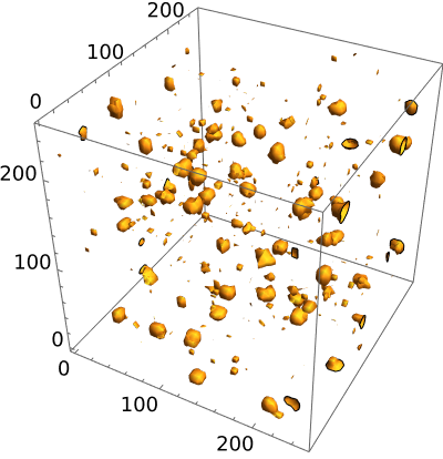
As the inflaton condensates begin to fragment, numerous regions of energy concentration gradually emerge. These regions account for a large portion of the energy of the inflaton condensate and keep oscillating with the same frequency. Such structures, the so-called oscillons, exhibit a stable profile and survive millions of oscillations. They usually form in a kind of potential models similar to what we chose with an expansion of a quadratic term near the origin and plateau near the large field value Amin et al. (2012); Lozanov and Amin (2018); Hasegawa and Hong (2018); Mahbub and Mishra (2023); Kawasaki et al. (2020); Liu et al. (2018); Sang and Huang (2021). We can observe the oscillons in the simulation results through snapshot of the spatial distribution of energy density after the fully formation of oscillons, as shown in Fig. 4.
The oscillon profile, a spherically symmetric structure with a time-varying peak in its center, has been well discussed in Sec. IV. The phenomena observed in the lattice confirms our results that the highlight region of the energy density is flashing with time, corresponding to changes in the amplitude of the core of the field configuration in the oscillon profile.


VI.1.2 equation of state and energy transfer


The equation of state is depicted by the blue curve in the top left and top right panels of Fig. 5 for T and E models, respectively. In both models, starts with a violent oscillation in the initial stage and then show a rapid damping, during which oscillons begin to emerge and form. The asymptotically approaching 0 of is corresponding to process that inflaton condensate fragment into oscillons. After the fully formation of oscillons, the curve of keeps slightly oscillating around . Oscillons behave as pressureless dust with and dominate the energy density of the universe for millions of oscillations.
The equation of state approaches slowly but not immediately, the reason of which is that the energy not stored inside the oscillons completely, but also in the relativistic mode Lozanov and Amin (2018). However it will take no longer than one -fold of expansion for because the energy stored in the relativistic modes redshifts as while oscillons behave like matter Lozanov and Amin (2018).
The changing of the energy components is depicted in the bottom left and bottom right panels of Fig. 5 for T and E models, respectively. The orange, purple and green curves represent the kinetic energy, potential energy and gradient term of the inflaton field, respectively. The energy of each component decreases as the universe expands throughout the process. Once the fragmentation begins, the gradient term of the field is sharply amplified and reach its peak value, leading to a breakdown of system’s adiabatic state Kasuya et al. (2003). A large number of adiabatic particle oscillons are generated in every oscillation until the gradient term satisfies adiabatic conditions. Subsequently, these three energy components are continuously converted into each other and eventually reach a stable ratio when the oscillons are fully formed and stabilized.
While the condensate rapidly decays and breaks up, most of the energy component is transferred into oscillons. Simultaneously, a small amount of energy is redshifted into relativistic mode and gradually becomes negligible as a result of the expansion of universe. The above process occurs almost simultaneously and complete in less than one -fold of expansion.
VI.2 Transient ()
Next we will focus on the case of parameter . As depicted by three different colored curves for the three values of the parameters , , in the Fig. 1, the potential shape in the bottom () are influenced by the parameters . As the parameter increases, the bottom region become flat and wide. The plateau regions () where the self-resonance happens and the slow roll inflation ends are not significantly changed by . In this paper, we take as an example for -attractor T and E models, and show the results of lattice simulations, which has not been investigated in the previous literature. The parameters and initial conditions in the simulation are listed in the third and fourth rows of Table. 1.
VI.2.1 back-reaction and structures form
Both T and E models exhibit intriguing phenomena in the simulations. The back-reaction on the inflaton condensates become apparent during the evolution. Some interconnected structures gradually formed, which is the same as the process of the back-reaction of oscillon cases (). Subsequently the condensates fragment into another interesting nonlinear structure, which is called transient Lozanov and Amin (2018, 2019).


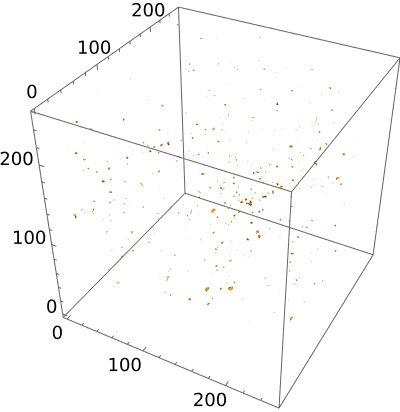
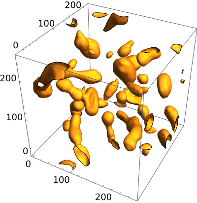
As shown in Fig. 6, transients form as soon as the fragmentation of the inflaton condensates begin. These structures exhibit approximately symmetric patterns and do not oscillate with time. Throughout the process, their spatial positions remain nearly constant in the lattice. Initially, these regions of high energy density are extensive, but they subsequently decay and gradually transform into smaller individual structures. Ultimately, only a few remnants persist within the lattice.
The phenomenon shown in lattice simulation is consistent with the results obtained from our small amplitude analysis. During preheating, the amplitudes of the perturbation is rapidly amplified due to parametric resonance, leading to rapid convergence and clustering of field structures. Subsequently, as the universe expands, these perturbations are swiftly smoothed out, causing the aggregated structure to disintegrate into a myriad of fragments.
VI.2.2 equation of state and energy transfer
The equation of state is depicted in the top left and top right panels of Fig. 7 for T and E models, respectively. After the fragmentation of the condensates, oscillate around for a very brief moment. Subsequently begins to approach with the decay of transients. The entire process occurs within less than one -fold of expansion. The equation of state is approximated to that of radiation dominance in the process of transient decay and fragmentation. The equation of state in the transients case () is significantly different from the case of oscillons (), as shown in Fig. 5.
As depicted in the second row of Fig. 7, all of the energy stored declines as a result of the universe’s expansion. The decrease in gradient term here occurs at a slower rate compared to other energy components and the gradient energy even surpasses potential energy after the moment of transient decay.
From the simulation of the -attractor models, we find that the nonlinear dynamical behavior of the inflaton field during the preheating phase exhibits similarities in both the symmetric T model and the asymmetric E model. The interesting nonlinear structures will be generated in both models, leading to the equation of state of the universe for parameter and for parameter .
VII Simulation of monodromy models
In this section, we will show the results of lattice simulation for monodromy model. The shape of the potential is shown in Fig. 1. In the region near the bottom, the potential is given by
| (24) |
While in the region of , the potential is approximated by
The model in the small field region depends on both and , depend only on in large field region. The values of parameters using in the simulation is listed in Table. 2.
| model | n | q | M | |
|---|---|---|---|---|
| monodromy model | 1 | 1 | 0.01 | 0.6 |
| monodromy model | 1.5 | 1 | 0.01 | 0.71 |
| monodromy model | 1.5 | 0.75 | 0.01 | 0.56 |
| monodromy model | 1.5 | 0.5 | 0.01 | 0.42 |
| monodromy model | 1.5 | 0.25 | 0.01 | 0.31 |
| monodromy model | 2 | 0.5 | 0.01 | 0.42 |
VII.1 structures form
Similar to the and cases in -attractor models, the parameter affects the formation of nonlinear structures in monodromy models. For example, if taking , in the region of and in the region of . Fig. 8 show the simulation of and cases in monodromy models, which are corresponding to the formation of oscillons and transients after the inflaton condensates fragmentation, respectively.


VII.2 effect of parameters and
We study the effect of parameters and on the nonlinear evolution by the simulations of different parameter values, see Table. 2. To investigate the impact of parameter , we fix parameter and run the simulation for , , . As the parameter increases, the end time of slow roll inflation occurs at larger field values, see the values in Table. 2, which gives a larger initial amplitude of the oscillating sclar field. The back-reaction on inflaton condensates will occur at a later time. Therefore, as the parameter increases, the decay of inflaton field and subsequent nonlinear process are delayed.
Fig. 9 shows the evolution of transients in the three cases of parameter and , , . The snapshot is taken at the time before the formation, after the full formation and when the decay of transients. The lifetime of the transient can be defined as -folds between the fragmentation of the inflaton condensates and the completely decay of the transient. In the simulation, we find that the lifetime of transients are roughly equal for different , around one -fold. From the scale factors given in Fig. 9, the lifetime of transients are for , respectively. Hence, the parameter has limited influence on the lifetime of the transient.
The first row in Fig. 10 depicts the evolution of the equation of state for three different value of parameters . In all three cases, the universe finally approaches to a radiation dominated state with the equations of state to be . As the parameter decreases, the duration required to achieve a radiation-dominated universe is significantly reduced. The second row in Fig. 10 shows the energy components. As the parameter decreases, all of the energy components show a slight increase after the condensate fragment.


Besides, we explore the effect of the parameter by comparing the simulations of parameters and parameters . Fig. 11 shows the results of the simulation for parameters . Through the calculation, the lifetime of the transient in the case of parameter is , which is shorter than that in (). Therefore, the parameter has significant influence on the lifetime of the transient. With the parameter increasing, lifetime of the transient is largely reduced.
As depicted in Fig. 12, the duration during which the equation of state approaches radiation dominance is shorter and the magnitudes of all energy components are relatively lower for than those . This is consistent with the result of the Floquet analysis that an increase in the parameter will reduce the resonance slightly.


VIII Conclusion and discussion
In this paper, we investigated the nonlinear dynamics of the inflaton field during preheating in the -attractor T model, E model and monodromy model, which are favored by the observations. These models have a power-law form near the origin () and a plateau in the region of . We presented the results of Floquet analysis in monodromy models and found that the potential parameters have a significant influence on the region of resonance bands, but have a weak influence on the resonance strength. Utilizing the small amplitude analysis method, we derived the analytical expression of the oscillons profile () for the -attractor T model and discussed the method applicability to the transient situations (). Through the (3+1) dimensional lattice simulation, we performed a detailed analysis of the dynamic evolution and the nonlinear structure during preheating in all three models. In the -attractor models, symmetric potential in T model and the asymmetric potential in E model lead to similar nonlinear dynamics. We also find that with the increase of the potential parameter in monodromy model, the lifetime of the transient is largely reduced, but the potential parameter has limited influence on the lifetime of the transient.
With the different combinations of the parameters and , we have investigated the influence of models parameters on the preheating. The parameters is only appear in the monodromy models. It mainly controls the region that . In our simulation, we find that back-reaction process will be later with the parameters increases, but the lifetime of the transients we calculate in the simulations is almost unchanged. While the parameter appear in three models only controls the phase of preheating that inflaton condensate fragment into oscillon () or transients (). As it increase, the lifetime of the transient from the fragmentation of the condensate to its decay of completely will be shorter. Compare to the parameters , the effect of is more significant.
Note that such structures, oscillons and transients, can be generated under arbitrary parameter we selected. Therefore, we expect that such structures will exist in all of the models with a wider the parameter range. Besides, the phases of formation and decay of these structures can generate the gravitional waves, and whether difference combinations of parameter will influence their frequency or energy density remains an open question. We will stress these issues in the future work.
IX Acknowledgement
We would like to thank Shulan Li, Qingyang Wang and Shoupan Liu for helpful discussions. This work is supported by the National Natural Science Foundation of China (Grant Nos. 12005184, 12175192, and 12005183).
References
- Aghanim et al. (2020) N. Aghanim et al. (Planck), “Planck 2018 results. VI. Cosmological parameters,” Astron. Astrophys. 641, A6 (2020), [Erratum: Astron.Astrophys. 652, C4 (2021)], arXiv:1807.06209 [astro-ph.CO] .
- Akrami et al. (2020) Y. Akrami et al. (Planck), “Planck 2018 results. X. Constraints on inflation,” Astron. Astrophys. 641, A10 (2020), arXiv:1807.06211 [astro-ph.CO] .
- Cai et al. (2015) Rong-Gen Cai, Zong-Kuan Guo, and Shao-Jiang Wang, “Reheating phase diagram for single-field slow-roll inflationary models,” Phys. Rev. D 92, 063506 (2015), arXiv:1501.07743 [gr-qc] .
- Cook et al. (2015) Jessica L. Cook, Emanuela Dimastrogiovanni, Damien A. Easson, and Lawrence M. Krauss, “Reheating predictions in single field inflation,” JCAP 04, 047 (2015), arXiv:1502.04673 [astro-ph.CO] .
- Kabir et al. (2019) R. Kabir, A. Mukherjee, and D. Lohiya, “Reheating constraints on Kähler moduli inflation,” Mod. Phys. Lett. A 34, 1950114 (2019), arXiv:1609.09243 [gr-qc] .
- Martin et al. (2015) Jerome Martin, Christophe Ringeval, and Vincent Vennin, “Observing Inflationary Reheating,” Phys. Rev. Lett. 114, 081303 (2015), arXiv:1410.7958 [astro-ph.CO] .
- German et al. (2024) Gabriel German, Juan Carlos Hidalgo, and Luis E. Padilla, “Inflationary models constrained by reheating,” Eur. Phys. J. Plus 139, 302 (2024), arXiv:2310.05221 [astro-ph.CO] .
- Hindmarsh and Salmi (2008) Mark Hindmarsh and Petja Salmi, “Oscillons and domain walls,” Phys. Rev. D 77, 105025 (2008), arXiv:0712.0614 [hep-th] .
- Enqvist et al. (2002) Kari Enqvist, Shinta Kasuya, and Anupam Mazumdar, “Inflatonic solitons in running mass inflation,” Phys. Rev. D 66, 043505 (2002), arXiv:hep-ph/0206272 .
- Coleman (1985) Sidney R. Coleman, “Q-balls,” Nucl. Phys. B 262, 263 (1985), [Addendum: Nucl.Phys.B 269, 744 (1986)].
- Frolov (2008) Andrei V. Frolov, “DEFROST: A New Code for Simulating Preheating after Inflation,” JCAP 11, 009 (2008), arXiv:0809.4904 [hep-ph] .
- Amin et al. (2019) Mustafa A. Amin, Jiji Fan, Kaloian D. Lozanov, and Matthew Reece, “Cosmological dynamics of Higgs potential fine tuning,” Phys. Rev. D 99, 035008 (2019), arXiv:1802.00444 [hep-ph] .
- Karam et al. (2023) Alexandros Karam, Niko Koivunen, Eemeli Tomberg, Antonio Racioppi, and Hardi Veerm”ae, “Primordial black holes and inflation from double-well potentials,” JCAP 09, 002 (2023), arXiv:2305.09630 [astro-ph.CO] .
- Guth (1981) Alan H. Guth, “The Inflationary Universe: A Possible Solution to the Horizon and Flatness Problems,” Phys. Rev. D 23, 347–356 (1981).
- Mukhanov and Chibisov (1981) Viatcheslav F. Mukhanov and G. V. Chibisov, “Quantum Fluctuations and a Nonsingular Universe,” JETP Lett. 33, 532–535 (1981).
- Starobinsky (1982) Alexei A. Starobinsky, “Dynamics of Phase Transition in the New Inflationary Universe Scenario and Generation of Perturbations,” Phys. Lett. B 117, 175–178 (1982).
- Linde (1983) Andrei D. Linde, “Chaotic Inflation,” Phys. Lett. B 129, 177–181 (1983).
- Linde (1990) Andrei D. Linde, “Particle physics and inflationary cosmology,” Contemp. Concepts Phys. 5, 1–362 (1990), arXiv:hep-th/0503203 .
- Albrecht et al. (1982) Andreas Albrecht, Paul J. Steinhardt, Michael S. Turner, and Frank Wilczek, “Reheating an Inflationary Universe,” Phys. Rev. Lett. 48, 1437 (1982).
- Kofman et al. (1994) Lev Kofman, Andrei D. Linde, and Alexei A. Starobinsky, “Reheating after inflation,” Phys. Rev. Lett. 73, 3195–3198 (1994), arXiv:hep-th/9405187 .
- Kofman et al. (1997) Lev Kofman, Andrei D. Linde, and Alexei A. Starobinsky, “Towards the theory of reheating after inflation,” Phys. Rev. D 56, 3258–3295 (1997), arXiv:hep-ph/9704452 .
- Amin et al. (2012) Mustafa A. Amin, Richard Easther, Hal Finkel, Raphael Flauger, and Mark P. Hertzberg, “Oscillons After Inflation,” Phys. Rev. Lett. 108, 241302 (2012), arXiv:1106.3335 [astro-ph.CO] .
- Kasuya et al. (2003) S. Kasuya, M. Kawasaki, and Fuminobu Takahashi, “I-balls,” Phys. Lett. B 559, 99–106 (2003), arXiv:hep-ph/0209358 .
- Amin (2010) Mustafa A. Amin, “Inflaton fragmentation: Emergence of pseudo-stable inflaton lumps (oscillons) after inflation,” (2010), arXiv:1006.3075 [astro-ph.CO] .
- Amin et al. (2010) Mustafa A. Amin, Richard Easther, and Hal Finkel, “Inflaton Fragmentation and Oscillon Formation in Three Dimensions,” JCAP 12, 001 (2010), arXiv:1009.2505 [astro-ph.CO] .
- Kawasaki et al. (2020) Masahiro Kawasaki, Wakutaka Nakano, and Eisuke Sonomoto, “Oscillon of Ultra-Light Axion-like Particle,” JCAP 01, 047 (2020), arXiv:1909.10805 [astro-ph.CO] .
- Mahbub and Mishra (2023) Rafid Mahbub and Swagat S. Mishra, “Oscillon formation from preheating in asymmetric inflationary potentials,” Phys. Rev. D 108, 063524 (2023), arXiv:2303.07503 [astro-ph.CO] .
- Sang and Huang (2021) Yu Sang and Qing-Guo Huang, “Oscillons during Dirac-Born-Infeld preheating,” Phys. Lett. B 823, 136781 (2021), arXiv:2012.14697 [hep-th] .
- Lozanov and Amin (2017) Kaloian D. Lozanov and Mustafa A. Amin, “Equation of state and duration to radiation domination after inflation,” Phys. Rev. Lett. 119, 061301 (2017).
- Lozanov and Amin (2018) Kaloian D. Lozanov and Mustafa A. Amin, “Self-resonance after inflation: oscillons, transients and radiation domination,” Phys. Rev. D 97, 023533 (2018), arXiv:1710.06851 [astro-ph.CO] .
- Liu et al. (2018) Jing Liu, Zong-Kuan Guo, Rong-Gen Cai, and Gary Shiu, “Gravitational Waves from Oscillons with Cuspy Potentials,” Phys. Rev. Lett. 120, 031301 (2018), arXiv:1707.09841 [astro-ph.CO] .
- Lozanov and Amin (2019) Kaloian D. Lozanov and Mustafa A. Amin, “Gravitational perturbations from oscillons and transients after inflation,” Phys. Rev. D 99, 123504 (2019).
- Liu et al. (2019) Jing Liu, Zong-Kuan Guo, Rong-Gen Cai, and Gary Shiu, “Gravitational wave production after inflation with cuspy potentials,” Phys. Rev. D 99, 103506 (2019), arXiv:1812.09235 [astro-ph.CO] .
- Hu et al. (2023) Wei-Yu Hu, Qing-Yang Wang, Yan-Qing Ma, and Yong Tang, “Gravitational Waves from Preheating in Inflation with Weyl Symmetry,” (2023), arXiv:2311.00239 [astro-ph.CO] .
- Zhou et al. (2013) Shuang-Yong Zhou, Edmund J. Copeland, Richard Easther, Hal Finkel, Zong-Gang Mou, and Paul M. Saffin, “Gravitational Waves from Oscillon Preheating,” JHEP 10, 026 (2013), arXiv:1304.6094 [astro-ph.CO] .
- Sang and Huang (2019) Yu Sang and Qing-Guo Huang, “Stochastic Gravitational-Wave Background from Axion-Monodromy Oscillons in String Theory During Preheating,” Phys. Rev. D 100, 063516 (2019), arXiv:1905.00371 [astro-ph.CO] .
- Hiramatsu et al. (2021) Takashi Hiramatsu, Evangelos I. Sfakianakis, and Masahide Yamaguchi, “Gravitational wave spectra from oscillon formation after inflation,” JHEP 03, 021 (2021), arXiv:2011.12201 [hep-ph] .
- Li et al. (2020) Junmei Li, Hongwei Yu, and Puxun Wu, “Production of gravitational waves during preheating in -attractor inflation,” Phys. Rev. D 102, 083522 (2020).
- Amin et al. (2018) Mustafa A. Amin, Jonathan Braden, Edmund J. Copeland, John T. Giblin, Christian Solorio, Zachary J. Weiner, and Shuang-Yong Zhou, “Gravitational waves from asymmetric oscillon dynamics?” Phys. Rev. D 98, 024040 (2018), arXiv:1803.08047 [astro-ph.CO] .
- Antusch et al. (2017) Stefan Antusch, Francesco Cefala, and Stefano Orani, “Gravitational waves from oscillons after inflation,” Phys. Rev. Lett. 118, 011303 (2017), [Erratum: Phys.Rev.Lett. 120, 219901 (2018)], arXiv:1607.01314 [astro-ph.CO] .
- Fu et al. (2019) Chengjie Fu, Puxun Wu, and Hongwei Yu, “Nonlinear preheating with nonminimally coupled scalar fields in the Starobinsky model,” Phys. Rev. D 99, 123526 (2019), arXiv:1906.00557 [astro-ph.CO] .
- Jin et al. (2020) Guoqiang Jin, Chengjie Fu, Puxun Wu, and Hongwei Yu, “Production of gravitational waves during preheating in the Starobinsky inflationary model,” Eur. Phys. J. C 80, 491 (2020), arXiv:2007.02225 [gr-qc] .
- Adshead et al. (2023) Peter Adshead, John T. Giblin, and Reid Pfaltzgraff-Carlson, “Kinetic Preheating after -attractor Inflation,” (2023), arXiv:2311.17237 [astro-ph.CO] .
- Adshead et al. (2024) Peter Adshead, John T. Giblin, and Avery Tishue, “Gravitational Waves from Kinetic Preheating,” (2024), arXiv:2402.16152 [astro-ph.CO] .
- El Bourakadi et al. (2021) K. El Bourakadi, M. Ferricha-Alami, H. Filali, Z. Sakhi, and M. Bennai, “Gravitational waves from preheating in Gauss–Bonnet inflation,” Eur. Phys. J. C 81, 1144 (2021), arXiv:2209.08581 [gr-qc] .
- Ueno and Yamamoto (2016) Yoshiki Ueno and Kazuhiro Yamamoto, “Constraints on -attractor inflation and reheating,” Phys. Rev. D 93, 083524 (2016), arXiv:1602.07427 [astro-ph.CO] .
- El Bourakadi et al. (2022) K. El Bourakadi, Z. Sakhi, and M. Bennai, “Preheating constraints in -attractor inflation and gravitational waves production,” Int. J. Mod. Phys. A 37, 2250117 (2022), arXiv:2209.09241 [gr-qc] .
- Eshaghi et al. (2016) Mehdi Eshaghi, Moslem Zarei, Nematollah Riazi, and Ahmad Kiasatpour, “CMB and reheating constraints to -attractor inflationary models,” Phys. Rev. D 93, 123517 (2016), arXiv:1602.07914 [astro-ph.CO] .
- Carrasco et al. (2015) John Joseph M. Carrasco, Renata Kallosh, and Andrei Linde, “Cosmological Attractors and Initial Conditions for Inflation,” Phys. Rev. D 92, 063519 (2015), arXiv:1506.00936 [hep-th] .
- Kallosh and Linde (2013) Renata Kallosh and Andrei Linde, “Universality Class in Conformal Inflation,” JCAP 07, 002 (2013), arXiv:1306.5220 [hep-th] .
- Galante et al. (2015) Mario Galante, Renata Kallosh, Andrei Linde, and Diederik Roest, “Unity of Cosmological Inflation Attractors,” Phys. Rev. Lett. 114, 141302 (2015), arXiv:1412.3797 [hep-th] .
- McAllister et al. (2010) Liam McAllister, Eva Silverstein, and Alexander Westphal, “Gravity Waves and Linear Inflation from Axion Monodromy,” Phys. Rev. D 82, 046003 (2010), arXiv:0808.0706 [hep-th] .
- McAllister et al. (2014) Liam McAllister, Eva Silverstein, Alexander Westphal, and Timm Wrase, “The Powers of Monodromy,” JHEP 09, 123 (2014), arXiv:1405.3652 [hep-th] .
- Silverstein and Westphal (2008) Eva Silverstein and Alexander Westphal, “Monodromy in the CMB: Gravity Waves and String Inflation,” Phys. Rev. D 78, 106003 (2008), arXiv:0803.3085 [hep-th] .
- Lin (2023a) Chia-Min Lin, “On the oscillations of the inflaton field of the simplest -attractor T-model,” Chin. J. Phys. 86, 323–331 (2023a), arXiv:2303.13008 [hep-ph] .
- Lozanov (2019) Kaloian D. Lozanov, “Lectures on Reheating after Inflation,” (2019), arXiv:1907.04402 [astro-ph.CO] .
- Amin et al. (2014) Mustafa A. Amin, Mark P. Hertzberg, David I. Kaiser, and Johanna Karouby, “Nonperturbative Dynamics Of Reheating After Inflation: A Review,” Int. J. Mod. Phys. D 24, 1530003 (2014), arXiv:1410.3808 [hep-ph] .
- Turzyński and Wieczorek (2019) Krzysztof Turzyński and Michał Wieczorek, “Floquet analysis of self-resonance in single-field models of inflation,” Phys. Lett. B 790, 294–302 (2019), arXiv:1808.00835 [astro-ph.CO] .
- Antusch et al. (2018) Stefan Antusch, Francesco Cefala, Sven Krippendorf, Francesco Muia, Stefano Orani, and Fernando Quevedo, “Oscillons from String Moduli,” JHEP 01, 083 (2018), arXiv:1708.08922 [hep-th] .
- Fodor et al. (2006) Gyula Fodor, Peter Forgacs, Philippe Grandclement, and Istvan Racz, “Oscillons and Quasi-breathers in the phi**4 Klein-Gordon model,” Phys. Rev. D 74, 124003 (2006), arXiv:hep-th/0609023 .
- Farhi et al. (2008) E. Farhi, N. Graham, Alan H. Guth, N. Iqbal, R. R. Rosales, and N. Stamatopoulos, “Emergence of Oscillons in an Expanding Background,” Phys. Rev. D 77, 085019 (2008), arXiv:0712.3034 [hep-th] .
- Fodor et al. (2008) Gyula Fodor, Péter Forgács, Zalán Horváth, and Árpád Lukács, “Small amplitude quasibreathers and oscillons,” Phys. Rev. D 78, 025003 (2008).
- Hertzberg (2010) Mark P. Hertzberg, “Quantum Radiation of Oscillons,” Phys. Rev. D 82, 045022 (2010), arXiv:1003.3459 [hep-th] .
- Hasegawa and Hong (2018) Fuminori Hasegawa and Jeong-Pyong Hong, “Inflaton fragmentation in E-models of cosmological -attractors,” Phys. Rev. D 97, 083514 (2018), arXiv:1710.07487 [astro-ph.CO] .
- Amin and Shirokoff (2010) Mustafa A. Amin and David Shirokoff, “Flat-top oscillons in an expanding universe,” Phys. Rev. D 81, 085045 (2010).
- Amin (2013) Mustafa A. Amin, “K-oscillons: Oscillons with noncanonical kinetic terms,” Phys. Rev. D 87, 123505 (2013), arXiv:1303.1102 [astro-ph.CO] .
- Manton and Romańczukiewicz (2023) N. S. Manton and T. Romańczukiewicz, “Simplest oscillon and its sphaleron,” Phys. Rev. D 107, 085012 (2023), arXiv:2301.09660 [hep-th] .
- Child et al. (2013) Hillary L. Child, John T. Giblin, Jr, Raquel H. Ribeiro, and David Seery, “Preheating with Non-Minimal Kinetic Terms,” Phys. Rev. Lett. 111, 051301 (2013), arXiv:1305.0561 [astro-ph.CO] .
- Felder and Tkachev (2008) Gary N. Felder and Igor Tkachev, “LATTICEEASY: A Program for lattice simulations of scalar fields in an expanding universe,” Comput. Phys. Commun. 178, 929–932 (2008), arXiv:hep-ph/0011159 .
- Lin (2023b) Chia-Min Lin, “The average equation of state for the oscillating inflaton field of the simplest -attractor E-model,” (2023b), arXiv:2305.01159 [hep-ph] .
- Greene et al. (1997) Patrick B. Greene, Lev Kofman, Andrei D. Linde, and Alexei A. Starobinsky, “Structure of resonance in preheating after inflation,” Phys. Rev. D 56, 6175–6192 (1997), arXiv:hep-ph/9705347 .
- Kallosh et al. (2013) Renata Kallosh, Andrei Linde, and Diederik Roest, “Superconformal Inflationary -Attractors,” JHEP 11, 198 (2013), arXiv:1311.0472 [hep-th] .
- Krajewski et al. (2019) Tomasz Krajewski, Krzysztof Turzyński, and Michał Wieczorek, “On preheating in -attractor models of inflation,” Eur. Phys. J. C 79, 654 (2019), arXiv:1801.01786 [astro-ph.CO] .
- Krajewski and Turzyński (2022) Tomasz Krajewski and Krzysztof Turzyński, “(P)reheating and gravitational waves in -attractor models,” JCAP 10, 005 (2022), arXiv:2204.12909 [astro-ph.CO] .