Nonequilibrium Induced Molecular Quantum Coherence Drives Magnetic Ordering in Coordination Compounds

Engineering magnetism at the atomic scale has emerged as one of the most vibrant, interesting and challenging areas of study in the field of condensed matter in the last decade. Fuelled by novel experimental techniques developed in the context of scanning tunneling microscopy (STM), scientists have been empowered to manipulate, control and probe matter at atomic scale resolution Chen (2007); Eigler, M and Scweizer, K (1990). The manipulation of atomic spins has yet captured much of the focus and efforts in experimental nanotechnology Loth et al. (2012); Khajetoorians et al. (2012); Heinrich et al. (2013). Driven by the need to produce novel quantum states of matter optimal for the use in quantum information and quantum engineering applications as well as for emergent spintronic technology Heinrich et al. (2015); Bogani and Wernsdorfer (2009); Urdampilleta et al. (2011), it is desired to tune spin-spin interactions to either ferromagnetic or to antiferromagnetic alignment Khajetoorians et al. (2012); Wagner et al. (2013) with stable single spin anisotropy.

The magnetic interactions, both in sign and magnitude, which respectively provide ferro- or antiferromagnetic couplings between spins, as well as magnetic anisotropies, can be adjusted through indirect spin interactions by properly orienting and separating the magnetic ions in the molecule being adsorbed Khajetoorians et al. (2012). On the other hand, the indirect interactions are completely determined by the electronic structure of the substrate, what suggests that engineering the density of states of the host will influence the sign and magnitude of the effective exchange coupling among the spins grafted onto it through the Kondo interaction Khajetoorians et al. (2012); Wagner et al. (2013); Khajetoorians et al. (2011); Simon et al. (2011).

By invoking the results in Koole et al. (2015); Jianlong Xia, Brian Capozzi, Sujun Wei, Mikkel Strange, Arunabh Batra, Jose R. Moreno, Roey J. Amir, Solomon et al. (2015); Tsuji et al. (2016); Fracasso et al. (2011); Pedersen et al. (2015), the transport properties of molecular junctions, particularly the (differential) conductance, can be hindered or enhanced depending on the nature and origin of quantum interference present within the molecular structure of interest. A manifestation of this has been shown to be intimately related with the conjugation order of the molecule, whether broken, cross or linear Bergfield and Stafford (2009); Valkenier et al. (2014); Guédon et al. (2012), and its bonding position with the electrodes or with the linking group, weather para, meta or ortho Pedersen et al. (2015).

Theoretical predictions have confirmed the observed low conductance in junctions under the influence of destructive quantum interference or even in the presence of quantum decoherence Saygun et al. (2016); Jaramillo and Fransson (2017), which is a condition that as well arises in magnetic tunneling junctions of a dimer of spins resembling the experiment reported in Urdampilleta et al. (2011), when both units are anti-ferromagnetically coupled. Following the same logic, it should in principle be possible to engineer spin-spin interactions in magnetic tunneling junctions by controlling the degree of quantum interference and the emergence of electronic decoherence allowed by the density of electron states, both in sign and magnitude. Here, the fully anti-ferromagnetic interaction is expected to localize the electron states in each energy level available for occupation whereas the fully ferromagnetic interaction is expected to delocalized the electron wave in the molecule, hence, favoring quantum coherence of different nature Saygun et al. (2016).

In this context, according to the work of Sharples et al. (2014); Wu et al. (2017); Grindell et al. (2016); Khajetoorians et al. (2012) where frustrated spin geometries have been engineered, completely ferromagnetic ordered, have been tailored, investigations on the effect of electronic quantum coherence and the emergence of decoherence is of great relevance and impact for the studies of open questions in atomic magnetism and in designing building blocks for quantum engineering systems. These issues pose giant challenges for experiments and theory.

The above arguments converge in the grounds of tailoring effective spin ordering by the coordinated action of gate and bias potentials, giving rise of what we call the magnetic $V_{\text{SD}}$–$V_{\text{G}}$ diagram. Subsequently these interactions can be probed using all-electrical measurements as predicted in Fransson et al. (2014), a completely unexplored issue both from the perspective of non-equilibrium nanophysics and from the point of view of nanotechnology and manipulation at the atomic scale.

Here, in the present work, we consider a trimer of magnetic ions immersed in an organic molecule that can be a phthalocyanine, a metal hydride such as M-porphyrin, where M denotes a transition metal element, or an organometal Jaramillo and Fransson (2017); Saygun et al. (2016), exhibiting the possibility of quantum interference whether destructive or constructive. The magnetic ions, which display a localized magnetic moment, do not interact directly, but only through the electron interactions in the host molecule, therefore, the spin-spin interactions are tuned via the molecular electronic structure. The magnetic ion-molecule system is adsorbed onto a metallic substrate, and then probed by a metallic STM tip. As such the Hamiltonian of the system STM–magnetic ion–molecule–substrate is given by:

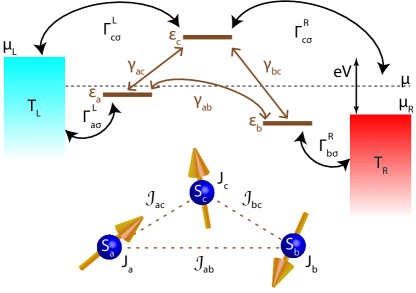
The system described through the Hamiltonian given in Eq. (1), is illustrated in Fig. 1.

In the model presented by Eq. (1), $\mathcal{H}_{tip}$ represents the Hamiltonian of the metallic tip, $\mathcal{H}_{sust}$ the Hamiltonian for the metallic substrate, $\mathcal{H}_{mol}$ is the molecular Hamiltonian, the local interaction between the magnetic ion and the conduction electrons is given by $\mathcal{H}_{sd}$ and the Tip-Molecule and Substrate-Molecule hybridization are given by Hamiltonians $\mathcal{H}_{tip-mol}$ and $\mathcal{H}_{subst-mol}$. The parameters defined in the model Hamiltonian are defined as follows: $\epsilon_{\bm{k}\sigma}(t)$ and $\epsilon_{\bm{q}\sigma}(t)$ are the energy bands of the metallic tip and the metallic substrate respectively, $\epsilon_{m\sigma}$ is the energy of the $m-th$ molecular orbital, $J_{m}$ is the Kondo coupling between the $m-th$ spin moment of the electron with energy $\epsilon_{m\sigma}$ and the $m-th$ localized spin moment denoted as $\bm{S}_{m}(t)$, and, $v_{m\bm{k}\sigma}(t)$ and $v_{m\bm{q}\sigma}(t)$ are the overlap integrals between wave functions from the tip and the molecule, and the substrate and the molecule respectively.

The Green’s function for the model represented by Eq. (1), can be obtained from the inverse of the retarded Green’s function given by expression 58. By inverting equation 59, the retarded Green’s function is evaluated, and the lesser and greater Green’s functions are obtained from

where $\epsilon$ and $\omega$ are related through $\epsilon=\hbar\omega$ and $\chi$ indexes the lead, whether $\alpha$ for the left lead, or $\beta$ for the right lead. In Eq. (2), the matrix $\bm{\Gamma}^{(\chi)}_{\sigma}$ is proportional to the imaginary part of the retarded self-energy $\bm{\Sigma}^{(\chi)R}_{\sigma}$ which can be paramterized by (see appendix A)

Here, $\bm{\Lambda}_{\sigma}^{(\chi)}$ is related to the Lamb-Shift Esposito et al. (2015a, b) and $\bm{\Gamma}_{\sigma}^{(\chi)}$ represent the coupling between the leads and the molecular energy levels. The diagonal matrix elements of the latter stands for the level broadening, and the off-diagonal matrix elements are related to the dephasing among levels coupled to the reservoir Jauho et al. (1994); Bedkihal and Segal (2012); Matityahu et al. (2013); Tu et al. (2014). To determine the form of matrix element $\bm{\Gamma}^{(\chi)}_{mn\sigma}$, we consider the definition from Jauho et al. (1994) of the retarded self-energy matrix element:

In the above expression, the couplings $v_{m\bm{k}\sigma}$ and $v_{n\bm{k}\sigma}^{*}$ appearing in the model Hamiltonians given by Eqs. (1f) and (1g), are complex in nature, and therefore, we can express both of them as an amplitude times a phase factor of the form $v_{m\bm{k}\sigma}=\left|v_{m\bm{k}\sigma}\right|e^{-i\phi_{m}}$ and $v_{m\bm{k}\sigma}^{*}=\left|v_{m\bm{k}\sigma}\right|e^{i\phi_{m}}$, to transform Eq. (4) into

From Eq. (5), we thus, define the elements $\Gamma^{(\chi)}_{mn\sigma}$ according to

where phases $\phi_{m}$ and $\phi_{n}$ determine the strength of the dephasing between levels $m$ and $n$. Moreover, it becomes crucial to determine the density of electron states $\bm{\rho}_{c}(\omega)$ in the quest for an understanding on what is the interplay between electronic structure and magnetism in the sample. The former can be obtained from the equation

and similarly, the spin density of states

In addition to the latter, it is often useful to think about magnetic ordering and change in magnetic configuration in terms of magnetic entropy and the corresponding energy flow, which holds intimacy with the symmetry of the system through which flows. By invoking the von Neuman entropy $\bm{\mathcal{S}}_{\sigma}$ P. (2007) given by

where $\bm{\rho}_{\sigma}$ denotes the density matrix of the system, we can write, a general expression in terms of contour Green’s functions for the entropy associated with spin degrees of freedom can be written

The above formulation for the spin entropy derives from the von Neumann expression obtained from Eq. (9), where the density matrix has been defined with the aid of the contour ordered Green’s function $\bm{G}^{<}_{\sigma\sigma}(\omega)$ in matrix form

Here we approach the question of the emergence of quantum interference and its relationship to the spin configuration of the molecule of interest. A useful theoretical tool available from the Landauer formalism Jauho et al. (1994) to determine the degree of quantum interference in a molecular conductor is the Transmission probability given by

From the same viewpoint, other theoretical tools such as particle and energy currents have lead to useful predictions in systems relevant for the discussion of the present paper Wagner et al. (2013); Saygun et al. (2016); Jaramillo and Fransson (2017), and therefore we have considered them into the investigation here reported. These transport quantities are written according to

where $\bar{\chi}$ refers to the lead on the opposite side to $\chi$ of the junction.

Along the same line, we study the quantum interference present in the molecule with regards of the trimmer spin structure with an analytic expression for the differential charge conductance $\bm{\sigma}^{\chi}=\partial J_{\chi}^{e}/\partial V$. This analytical observable is found to be given by (see appendix C):

Effective spin-spin interactions are calculated from the expression derived in ref. Fransson et al. (2014). Specifically, in this paper we address the effective Heisenberg exchange interactions present in the system described by the model given in Eq. (1) and illustrated in Fig. 1. These interactions among three localized magnetic moments labeled as $\bm{S}_{a}$, $\bm{S}_{b}$ and $\bm{S}_{c}$, that are coupled via Kondo interactions $J_{a}$, $J_{b}$, and $J_{c}$ with electrons present in three energy levels $\epsilon_{a}$, $\epsilon_{b}$ and $\epsilon_{c}$ respectively, are given by Eq. (63). Here, we pay special attention to two cases of great interest, which are the ferromagnetic state where all effective interactions $\bm{\mathcal{J}}_{mn}$ are negative, and the antiferromagnetic state where these interactions are now all positive. The stability and control of these ordering, as well as its manipulation and detection can be done by several means, one of them being the all-electrical control as demonstrated for Manganese based metal hydrides Osorio et al. (2010), among other experimental realizations Vincent et al. (2012); Aradhya and Venkataraman (2013); Urdampilleta et al. (2011); Krainov et al. (2017); Mannini et al. (2014). All-electrical control has also been shown to allow for atom by atom tailoring of nanomagnets Khajetoorians et al. (2012) thorugh the RKKY interaction including spin-frustrated networks. Moreover, all electrical control has provided a means of control for the singlet-triplet switching in a dimer of Cobalt atoms, and these states were detected by measurements of charge current flowing through the host molecule. In single magnetic unit molecules, important properties have been also engineered with the aid of a bias voltage. Another degree of control possible is the control through gate fields, demonstrated in the Anthraquinone transistor, in which case the destructive quantum interference exhibited by this type of molecule was lifted by the action of this gate Koole et al. (2015). The latter suggests that a combined bias voltage - gate field control scheme can provide the possibility to switch between spin states determined by the magnetic ordering present in the molecule, and the nature and strength of quantum interference have a strong chance to also play a role in this switching dynamics. The system we address here, combines these means of control, that is, the electric control provided by a bias voltage and control driven by the gate field, as well as the variation of the degree of quantum coherence present in the electronic part of the molecule. The latter is achieved by means of modulating the model given by Eq. (1) with associated Green’s function given by Eq. (59), in terms of the parameter $\gamma_{ab}$, which varies from $0$ to $6.0$ meV, where $\gamma_{ab}=0$ meV resembles a molecular structure with no possibility to exhibit quantum interference, and as $\gamma_{ab}$ increases, the degree of electronic coherence in the system increases. This way of controlling quantum interference in the multiple sites model in the electronic $\Lambda$–$\Delta$ system was studied in ref. Guédon et al. (2012). Here, we extend the investigation by considering a molecule with magnetic units, the question of atom by atom engineered exchange interaction and the interplay among the degree of electronic quantum interference and other means of control, namely a bias voltage and a gate field, in the switching dynamics of magnetic ordering in the molecule of interest. (See Fig. 1)

With the aim of visualising phase transitions in magnetic ordering of the trimmer, we study the effect of a symmetry breaking phenomenom induced by a Zeeman term in the effective spin-spin Heisenberg interaction Hamiltonian (62) by means of the spin expectation values given by (145). The new spin Hamiltonian is:

, where $\Delta$ is a constant equal to one in atomic units, and $\bm{B}_{k}$ are staggered fields for each localized spin. The isotropic nature of the Heisenberg effective interaction permits to project each localized spin along the z-direction in particular, without loose of generality, in order to characterize the phase transitions.

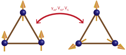
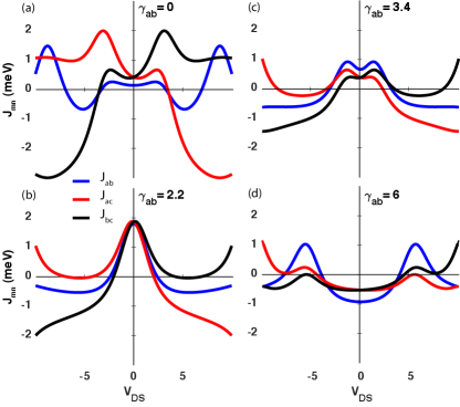
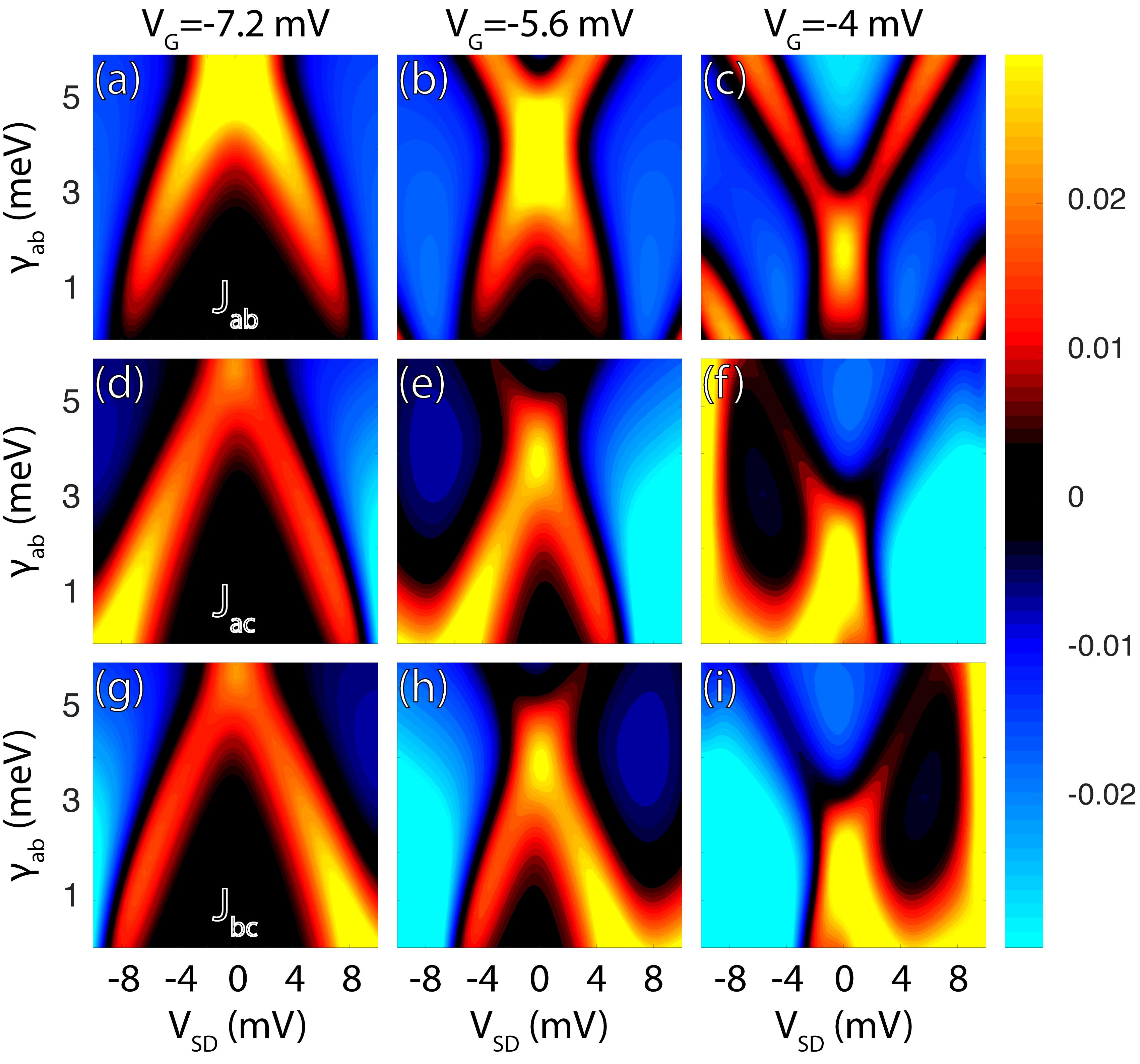
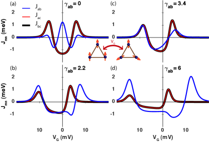
The voltage, electric field and delocalization induced switching dynamics of the spin ordering in the molecule of interest in the present paper is demonstrated here, by predicting the variation of the effective exchange interactions among the magnetic units present in the molecules, namely $\bm{\mathcal{J}}_{AB}$, $\bm{\mathcal{J}}_{AC}$ and $\bm{\mathcal{J}}_{BC}$. This variation is shown to be induced by the modulation of three different conditions driving the molecular degrees of freedom. First, parameter $\gamma_{ab}$ is varied in the range $0\leq\gamma_{ab}\leq 6$ meV. The variation of this parameter, induces a change in spin ordering in the molecule from nearly eight-fold-degeneracy and spin-frustrated state to all ferromagnetic ordering as depicted in the scheme shown in Fig. 2, and as predicted through the evaluation of $\bm{\mathcal{J}}_{AB}$, $\bm{\mathcal{J}}_{AC}$ and $\bm{\mathcal{J}}_{BC}$ shown in Fig. 3, and done by employing Eq. (63). Moreover, the contour shown in Fig. 4 illustrates how the modulation of $\gamma_{ab}$ has an effect on the spin ordering around zero-bias, for $3$ different values for the gate field expressed as an energy $V_{\text{G}}=-7.2$ mV, -5.6 mV, -4.0 mV. This figure, shows that around zero bias there is a commutation among quantum states with all anti-ferromagnetic spin-spin interactions to those with all ferromagnetic interactions among spins. For $V_{\text{G}}=-4.0$ mV, the frustrated spin state in the molecules occurs at lower values for the parameter $\gamma_{ab}$, as compare with other values for the gate field. At larger values of $\gamma_{ab}$ for the same gate field $V_{\text{G}}$, the spins align ferromagnetically.

The phenomenological insights and microscopic mechanisms behind the modulation of the parameter $\gamma_{ab}$, can be understood by considering the phenomenon of quantum interference in molecular junctions as discussed in Guédon et al. (2012), which investigates quantum coherent phenomena in molecular junction with a similar electronic configuration to the one investigated in this paper, with the differentiating factor of having the couplings $\Gamma^{(\chi)}_{C\sigma}$ for $\chi=\alpha,\beta$ exactly equal to zero.

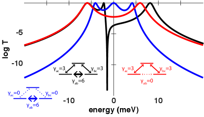
Under this assumption, the variation of $\gamma_{ab}$ from vanishing behavior to an intermediate value resembles the transition of the molecular structure corresponding to Anthracene-like (linear conjugation) molecular structure, to Anthraquinone-like (Cross-Conjugation) molecular structure where delocalization dominates the electronic processes within the molecule Guédon et al. (2012). From the electronic transmission probability calculated for the system of interest from Eq. (12), it can be shown that $\gamma_{ab}$ is associated with the ability for the system to exhibit electronic quantum interference as shown in Fig. 5, Valkenier et al. (2014).

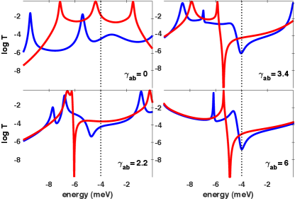
By considering the effect of the spin structure in the ability for the system to exhibit quantum interference, mainly of destructive nature, Fig. 6 shows that the ordering of the magnetic units in the trimmer has a decisive effect on the strength of the transmission dip, the broadening and the localization in energy, showing that the respective increase in magnetic symmetry is complained with the corresponding exhibition of weak quantum interference of destructive nature, and the corresponding decrease in symmetry, is associated with the lifting of coherence in the molecule.

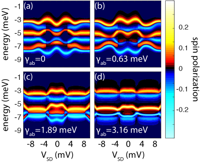
This particular feature of this system can be understood from considering the spin polarized density of states (see Fig. 7) around zero bias and through a bias window in which the system exhibits clear order. In this particular regime, the spin density of states presents abrupt changes when the order is lost, this around the set value for $V_{\text{G}}$.

An additional mean for controlling the ordering in the magnetic trimer is the bias voltage $V_{\text{SD}}$, which induces a non-equilibrium behavior in the system under study. An applied bias will as well induced an anti-ferromagnetic state in the spin trimer by an appropriate driving through the gate field of the molecule, and then, by swapping over a range of bias voltages, this state will be switched to an all ferromagnetic coupling configuration. This scheme of commutation is shown in Fig. 2.

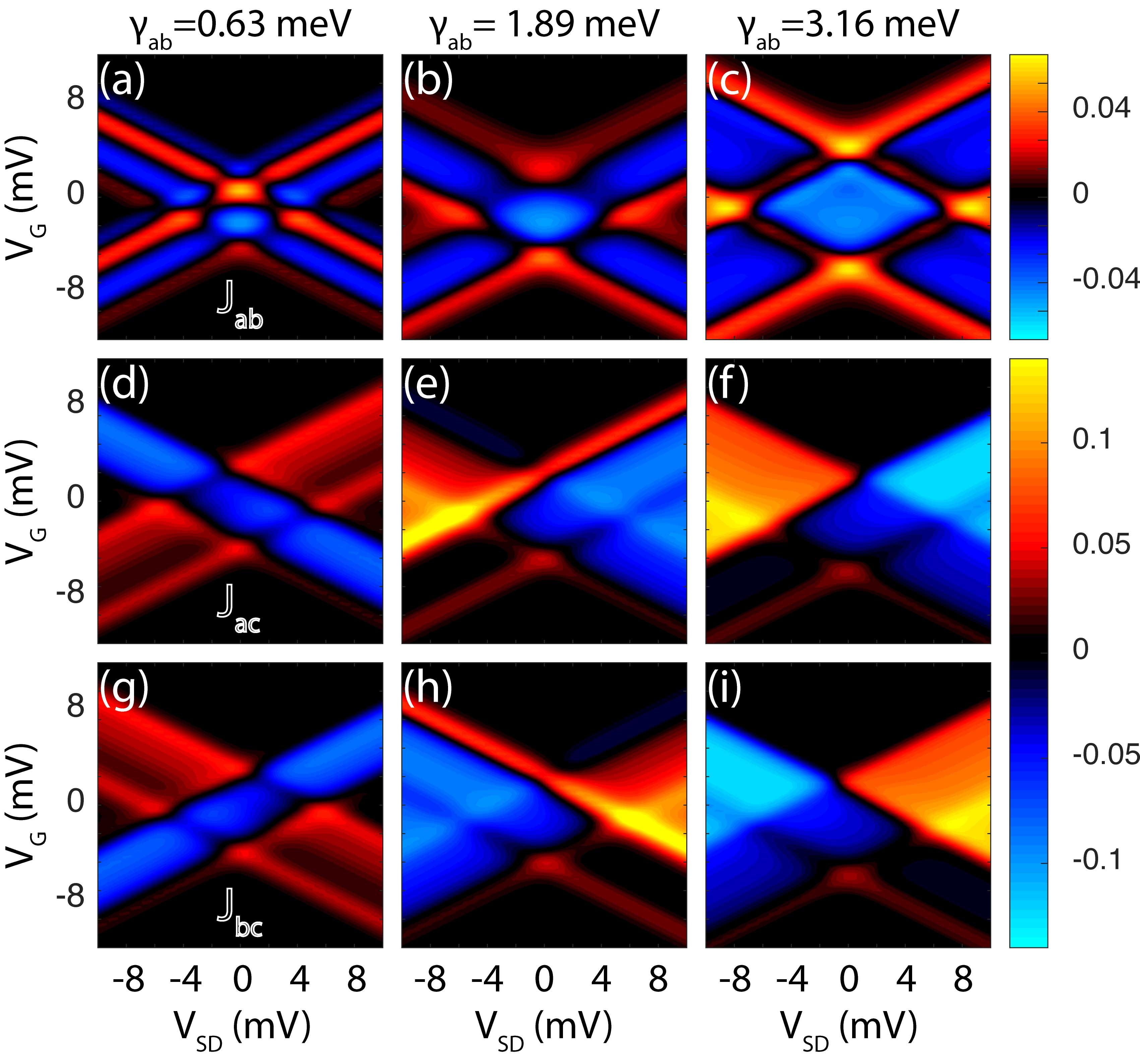
By staring at the contour plots in Fig. 8 it can be seen that there are regions in the $V_{\text{SD}}$–$V_{\text{G}}$ diagram for the effective exchange that correspond to one type of ordering and by the selecting biasing of the junction, a different state can be engineered, following the line of thought of the experiments reported in Loth et al. (2012); Heinrich et al. (2013, 2015); Khajetoorians et al. (2011, 2012); Jungwirth et al. (2016); Otte et al. (2009), where magnetic excitations in ad-atoms are engineered by the action of electric drives, in many cases in agreement with the RKKY limit. Here we have explored an additional degree of freedom for controlling this tailoring at the atomic scale, that is, the gate field $V_{\text{G}}$ which provides reasonable tuning possibility among anti-ferromagnetic (AFM) and ferromagnetic (FM) ones as shown in Fig. 9, hence empowering the optimal location of the operating point of the molecule in the magnetic $V_{\text{SD}}$–$V_{\text{G}}$ diagram. This means of control, as stated before, has been successfully demonstrated in Koole et al. (2015). Now, we will focus on what are the possibilities for tuning either anti-ferromagneticaly or ferromagnetically the magnetic units in the probed molecule. Fig. 9 considers the effective exchanges among spins as a function of gate voltage for a zero-bias condition. Therefore, this prediction cannot be verified by electrical means, though it provides some insight on how to tune the system with the gate field to commute among magnetic configurations, as exemplified in Fig. 2.

By looking now at Fig. 9, one sees the gating conditions for which the anti-ferromagnetic state will be more stable and robust against variations in the gate field and against modulations of the parameter determining the degree of quantum interference $\gamma_{ab}$, for which we determined this condition to be $V_{\text{G}}\approx-4.0$ mV. By changing the gating condition is possible to obtain the all-ferromagnetic configuration for small values of $\gamma_{ab}$, or this can be achieved by stabilizing the gate field around the set value, and rather modulating $\gamma_{ab}$ as shown in the lower right panel of Fig. 9; condition perfectly exemplified in the diagram shown in Fig. 2.

In the present paper, we are interested in two regimes of ordering: Ferromagnetic and Anti-Ferromagnetic. To determine whether the spin states exhibit classical correlations or quantum entanglement, we analyze the eigen-values and the corresponding eigen-state and the associated Von-Neumann entropy of the effective spin Hamiltonian 62. Let’s consider two relevant cases , where $\bm{\mathcal{J}}_{ab}=\bm{\mathcal{J}}_{ac}=\bm{\mathcal{J}}_{bc}=\bm{\mathcal{J}}$ and where $\bm{\mathcal{J}}_{ab}=\bm{\mathcal{J}}$, $\bm{\mathcal{J}}_{ac}=\bm{\mathcal{J}}_{bc}=\bm{\mathcal{J}}_{0}$, and determine the spectral diagram for the quantum spin states in both, the ferromagnetic and the anti-ferromagnetic spin ordering.

In the present reported work we considered a magnetic trimer, with a three level electronic system coupled with its hosted magnetic units via Kondo interaction, driven by a metallic tunneling junction, such that resembles a scanning tunneling microscopy experiment on magnetic ad-atoms on metallic surface. Additionally, the set up allows for an electric field acting as a gate drive, which in convergence with the bias voltage $V_{DS}$ define a magnetic $V_{DS}$–$V_{G}$ diagram where the symmetry status of the magnetic trimer becomes evident. We have shown that through the following three different mechanisms:

1. 1.

   Modulation of the nature and strength of the electronic quantum interference,

2. 2.

   Voltage bias induced non-equilibrium stationary dynamics,

3. 3.

   Gate field control of the electronic structure Koole et al. (2015)

a switching dynamics between all anti-ferromagnetic coupling spin state and all ferromagnetic one can be induced. Interestingly, the results reported for the indirect exchange interaction shown in Figs. 5,8,9, showed that not only the orientation but the relative strength or the order can be tuned in the magnetic $V_{DS}-V_{G}$ diagram for a variety of modulations of the parameter $\gamma_{ab}$, showing the corresponding of the magnetic formation with respect to the control means proposed in this work. Lastly, focusing on the objective of the study, which is to trace a correlation between ordering in the magnetic molecule and coherence in the electronic background, we infer from Fig. 6 that around the set Fermi level by the Gate field $V_{G}$ (dotted line in black), there is a controlled but prominent (Fano-like dip?) decay in the electronic transmission signing the emergence of the quantum interference of destructive nature. This conclusion, suggests that in the ferromagnetic induced delocalization, the ability to exhibit quantum interference dominates over the quantum coherent phenomena induced by the anti-ferromagnetic localization, in which case entropy driven processes will tend to be robust against anti-ferromagnetic induced electronic decoherence. This conclusion is in agreement with the predictions published in Jaramillo and Fransson (2017) with regards to the competition between singlet-triplet formation and orbital localization.

We would like to acknowledge M. Araujo, L. Nordström, P. Oppeneer, M. Pereiro, and Y. Sassa for useful discussions and feedback. We acknowledge funding from Minciencias (Ministry of Science, Technology and Innovation - Colombia) and From Universidad del Valle through the grant for the project with reference CI 71261 corresponding to the call by Minciencias No. 649 from 2019 for postdoctoral research scholars under the agreement number 80740-618-2020.

References

• Chen (2007) C. J. Chen, Introduction to Scanning Tunneling Microscopy (Oxford University Press, 2007), 3rd ed., ISBN 9780198856559.
• Eigler, M and Scweizer, K (1990) D. Eigler, M and E. Scweizer, K, Nature 344, 524 (1990).
• Loth et al. (2012) S. Loth, S. Baumann, C. P. Lutz, D. M. Eigler, and A. J. Heinrich, Science 335, 196 (2012), ISSN 10959203.
• Khajetoorians et al. (2012) A. A. Khajetoorians, J. Wiebe, B. Chilian, S. Lounis, S. Blügel, and R. Wiesendanger, Nature Physics 8, 497 (2012), ISSN 17452481, URL http://dx.doi.org/10.1038/nphys2299.
• Heinrich et al. (2013) B. W. Heinrich, L. Braun, J. I. Pascual, and K. J. Franke, Nature Physics 9, 765 (2013), ISSN 17452481, eprint 1405.6984.
• Heinrich et al. (2015) B. W. Heinrich, L. Braun, J. I. Pascual, and K. J. Franke, Nano Letters 15, 4024 (2015), ISSN 15306992, eprint 1412.7454.
• Bogani and Wernsdorfer (2009) L. Bogani and W. Wernsdorfer, Nanoscience and Technology: A Collection of Reviews from Nature Journals pp. 194–204 (2009).
• Urdampilleta et al. (2011) M. Urdampilleta, S. Klyatskaya, J. P. Cleuziou, M. Ruben, and W. Wernsdorfer, Nature Materials 10, 502 (2011), ISSN 14764660, URL http://dx.doi.org/10.1038/nmat3050.
• Wagner et al. (2013) S. Wagner, F. Kisslinger, S. Ballmann, F. Schramm, R. Chandrasekar, T. Bodenstein, O. Fuhr, D. Secker, K. Fink, M. Ruben, et al., Nature Nanotechnology 8, 575 (2013), ISSN 17483395, URL http://dx.doi.org/10.1038/nnano.2013.133.
• Khajetoorians et al. (2011) A. A. Khajetoorians, S. Lounis, B. Chilian, A. T. Costa, L. Zhou, D. L. Mills, J. Wiebe, and R. Wiesendanger, Physical Review Letters 106, 6 (2011), ISSN 00319007.
• Simon et al. (2011) E. Simon, B. Újfalussy, B. Lazarovits, A. Szilva, L. Szunyogh, and G. M. Stocks, Physical Review B - Condensed Matter and Materials Physics 83, 1 (2011), ISSN 10980121.
• Koole et al. (2015) M. Koole, J. M. Thijssen, H. Valkenier, J. C. Hummelen, and H. S. D. Zant, Nano Letters 15, 5569 (2015), ISSN 15306992, eprint 1507.08913.
• Jianlong Xia, Brian Capozzi, Sujun Wei, Mikkel Strange, Arunabh Batra, Jose R. Moreno, Roey J. Amir, Solomon et al. (2015) G. C. Jianlong Xia, Brian Capozzi, Sujun Wei, Mikkel Strange, Arunabh Batra, Jose R. Moreno, Roey J. Amir, Solomon, L. Venkataraman, and L. M. Campos, Nano Letters 15, 7177 (2015), ISSN 15306992.
• Tsuji et al. (2016) Y. Tsuji, R. Hoffmann, M. Strange, and G. C. Solomon, Proceedings of the National Academy of Sciences of the United States of America 113, E413 (2016), ISSN 10916490.
• Fracasso et al. (2011) D. Fracasso, H. Valkenier, J. C. Hummelen, G. C. Solomon, and R. C. Chiechi, Journal of the American Chemical Society 133, 9556 (2011), ISSN 00027863.
• Pedersen et al. (2015) K. G. Pedersen, A. Borges, P. Hedegård, G. C. Solomon, and M. Strange, Journal of Physical Chemistry C 119, 26919 (2015), ISSN 19327455.
• Bergfield and Stafford (2009) J. P. Bergfield and C. A. Stafford, Nano Letters 9, 3072 (2009), ISSN 15306984.
• Valkenier et al. (2014) H. Valkenier, C. M. Guédon, T. Markussen, K. S. Thygesen, S. J. Van Der Molen, and J. C. Hummelen, Physical Chemistry Chemical Physics 16, 653 (2014), ISSN 14639076.
• Guédon et al. (2012) C. M. Guédon, H. Valkenier, T. Markussen, K. S. Thygesen, J. C. Hummelen, and S. J. Van Der Molen, Nature Nanotechnology 7, 305 (2012), ISSN 17483395, eprint 1108.4357.
• Saygun et al. (2016) T. Saygun, J. Bylin, H. Hammar, and J. Fransson, Nano Letters 16, 2824 (2016), ISSN 15306992.
• Jaramillo and Fransson (2017) J. D. Jaramillo and J. Fransson, Journal of Physical Chemistry C 121, 27357 (2017), ISSN 19327455, eprint 1702.05389.
• Sharples et al. (2014) J. W. Sharples, D. Collison, E. J. McInnes, J. Schnack, E. Palacios, and M. Evangelisti, Nature Communications 5, 3 (2014), ISSN 20411723.
• Wu et al. (2017) Y. Wu, M. D. Krzyaniak, J. F. Stoddart, and M. R. Wasielewski, Journal of the American Chemical Society 139, 2948 (2017), ISSN 15205126.
• Grindell et al. (2016) R. Grindell, V. Vieru, T. Pugh, L. F. Chibotaru, and R. A. Layfield, Dalton Transactions 45, 16556 (2016), ISSN 14779234.
• Fransson et al. (2014) J. Fransson, J. Ren, and J. X. Zhu, Physical Review Letters 113, 1 (2014), ISSN 10797114, eprint 1401.5592.
• Esposito et al. (2015a) M. Esposito, M. A. Ochoa, and M. Galperin, Physical Review Letters 114, 1 (2015a), ISSN 10797114, eprint 1411.1800.
• Esposito et al. (2015b) M. Esposito, M. A. Ochoa, and M. Galperin, Physical Review B - Condensed Matter and Materials Physics 92, 1 (2015b), ISSN 1550235X.
• Jauho et al. (1994) A. P. Jauho, N. S. Wingreen, and Y. Meir, Physical Review B 50, 5528 (1994), ISSN 01631829.
• Bedkihal and Segal (2012) S. Bedkihal and D. Segal, Physical Review B - Condensed Matter and Materials Physics 85, 1 (2012), ISSN 10980121.
• Matityahu et al. (2013) S. Matityahu, A. Aharony, O. Entin-Wohlman, and S. Tarucha, New Journal of Physics 15 (2013), ISSN 13672630, eprint 1307.0228.
• Tu et al. (2014) M. W. Y. Tu, A. Aharony, W. M. Zhang, and O. Entin-Wohlman, Physical Review B - Condensed Matter and Materials Physics 90, 1 (2014), ISSN 1550235X, eprint 1406.6258.
• P. (2007) H. B. . F. P. P., The Theory of Open Quantum Systems, vol. 1 (Oxford University Press, 2007), 1st ed., ISBN 9781119130536.
• Osorio et al. (2010) E. A. Osorio, K. Moth-Poulsen, H. S. Van Der Zant, J. Paaske, P. Hedegård, K. Flensberg, J. Bendix, and T. Bjørnholm, Nano Letters 10, 105 (2010), ISSN 15306984.
• Vincent et al. (2012) R. Vincent, S. Klyatskaya, M. Ruben, W. Wernsdorfer, and F. Balestro, Nature 488, 357 (2012), ISSN 00280836, URL http://dx.doi.org/10.1038/nature11341.
• Aradhya and Venkataraman (2013) S. V. Aradhya and L. Venkataraman, Nature Nanotechnology 8, 399 (2013), ISSN 17483395, URL http://dx.doi.org/10.1038/nnano.2013.91.
• Krainov et al. (2017) I. V. Krainov, J. Klier, A. P. Dmitriev, S. Klyatskaya, M. Ruben, W. Wernsdorfer, and I. V. Gornyi, ACS Nano 11, 6868 (2017), ISSN 1936086X.
• Mannini et al. (2014) M. Mannini, F. Bertani, C. Tudisco, L. Malavolti, L. Poggini, K. Misztal, D. Menozzi, A. Motta, E. Otero, P. Ohresser, et al., Nature Communications 5, 1 (2014), ISSN 20411723, URL http://dx.doi.org/10.1038/ncomms5582.
• Jungwirth et al. (2016) T. Jungwirth, X. Marti, P. Wadley, and J. Wunderlich, Nature Nanotechnology 11, 231 (2016), ISSN 17483395, eprint 1509.05296, URL http://dx.doi.org/10.1038/nnano.2016.18.
• Otte et al. (2009) A. F. Otte, M. Ternes, S. Loth, C. P. Lutz, C. F. Hirjibehedin, and A. J. Heinrich, Physical Review Letters 103, 1 (2009), ISSN 00319007.
• H.J. Haug (2008) A. P. J. H.J. Haug, Quantum Kinetics in Transport and Optics of Semiconductors (Springer, Berlin, 2008), 2nd ed., ISBN 9783540735618.