Nonclassical Preparation of Quantum Remote States

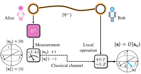
In the RSP protocol Pati00 ; Bennett01 , Alice and Bob initially share an Einstein-Podolsky-Rosen (EPR) pair $\ket{\Psi^{-}}=(\ket{01}-\ket{10})/\sqrt{2}$. Because of rotational symmetry the state $\ket{\Psi^{-}}$ can be rewritten as $\ket{\Psi^{-}}=(U\ket{\mathbb{s}_{0}}\otimes U\ket{\mathbb{s}_{0}^{\bot}}-U\ket{\mathbb{s}_{0}^{\bot}}\otimes U\ket{\mathbb{s}_{0}})/\sqrt{2}$ Cabello02 , where $\ket{\mathbb{s}_{0}}$ and $\ket{\mathbb{s}_{0}^{\bot}}$ are arbitrary pure states that constitute an orthonormal basis, and $U$ is an arbitrary single qubit unitary operator. If the quantum state, $\ket{\mathbb{s}}=(\ket{0}+e^{i\phi}\ket{1})/\sqrt{2}$, on the equatorial plane of the Bloch sphere, is the target state envisaged by Alice, she can measure her qubit in the basis $\{U\ket{\mathbb{s}_{0}},U\ket{\mathbb{s}_{0}^{\bot}}\}$ to prepare the state $\ket{\mathbb{s}}=U\ket{\mathbb{s}_{0}}$ for Bob. Depending on the outcome of Alice’s measurement, one classical bit (cbit) is sent from Alice to Bob in order to tell him whether or not he needs to apply a $\pi$ rotation about the $z$ axis for state preparation to be achieved. For example, the state $\ket{\mathbb{s}}$ can be remotely prepared by using the RSP protocol with $\ket{\mathbb{s}_{0}}=\ket{0}$ and a rotation operator $U$: $R(\phi)\!=\!(\ket{0}\!\!\bra{0}\!+\!e^{i\phi}\ket{1}\!\!\bra{0}\!+\!\ket{0}\!\!\bra{1}\!-\!e^{i\phi}\ket{1}\!\!\bra{1})\!/\!\sqrt{2}$. See Fig. 1.

The RSP confers the obvious advantage of remotely manipulating Bob’s qubit. In particular, if Bob is unable to locally implement the target operator $U$ but only the simple $\pi$ rotation, Alice can help. Moreover, compared to teleportation Bennett93 , which requires Bell-state measurements Pirandola15 for transmitting an unknown qubit, the RSP protocol only needs local measurements on Alice’s particle. These two features makes RSP appealing and well adapted for a range of applications in quantum information and quantum engineering — from deterministically creating single-photon states Jeffrey04 to preparing single-photon hybrid entanglement Barreiro10 , initializing atomic quantum memory Rosenfeld07 , and assisting teleportation between atomic-ensemble quantum nodes Bao12 .

Identifying truly quantum RSP, irreproducible by any classical means, is not only significant in its own right, but can be useful for realizing the power of quantum-enabled technologies in which RSP plays a role Jeffrey04 ; Barreiro10 ; Rosenfeld07 ; Bao12 . Validation of RSP naturally leads to the following fundamental question: what are the physical resources actually required to realize nonclassical RSP?

More recently, it was discovered that quantum discord Ollivier01 ; Zurek00 ; Henderson01 , which measures nonclassical correlations between two systems in terms of the difference between two prescribed expressions for mutual information, serves as a resource for RSP Dakic12 . While maximally-entangled EPR pairs are assumed to be the default states used in the ideal RSP protocol, rather remarkably, states with no entanglement can outperform entangled states in RSP once they possess non-zero geometric quantum discord Dakic10 ; Luo10 . Importantly, this kind of verification relies on assumptions deduced from quantum theory. It does not generally hold for practical implementations where experimental imperfections can be described by classical physics. The same assumption is made in the fidelity benchmarks for RSP Killoran10 , which offer a seminal paradigm for ruling out certain cheating strategies. This issue turns out to hinge on whether it is possible to simulate RSP using classical methods.

Driven by the desire to understand the resources necessary for the nonclassical preparation of quantum remote states, we investigate to what extent RSP can be performed with generic classical dynamical processes. We introduce a model to capture the classical dynamic change to a state which can occur as the result of a remote-state preparation process. The scenario considered in this model generally goes beyond the assumptions made in the existing verification methods Dakic12 ; Killoran10 . We show that certain RSPs based on quantum discord can be described by such classical processes. A new kind of EPR steering Wiseman07 ; Reid09 is found and proven to be necessary for surpassing such classical preparation of quantum remote states. This enables nonclassicality of experimental implementations to be measured in terms of quantum process steering, which we will introduce below. Experimental demonstration using polarization-correlated photon pairs support our theoretical predictions.

Theory.—The whole RSP process can be considered as a quantum operation, $\mathcal{E}_{\text{RSP}}$, implementing the following state transformation:

where $\rho_{\mathbb{s}_{0}}=\ket{\mathbb{s}_{0}}\!\!\bra{\mathbb{s}_{0}}$ is the initial state before the RSP process, and $\rho_{\mathbb{s}}=\ket{\mathbb{s}}\!\!\bra{\mathbb{s}}$ is the output state after the process occurs. It is worth emphasizing that RSP is nonclassical since $\mathcal{E}_{\text{RSP}}$ performs a unitary quantum-mechanical transformation $U$. Moreover, $\mathcal{E}_{\text{RSP}}$ comprises all the operations and resources required to implement the RSP protocol. Therefore, any experimental imperfections in these necessary elements can affect the realization of $\mathcal{E}_{\text{RSP}}$. The worst case scenario is when a real-world RSP process may be interpreted as a classical process.

To demonstrate our classical RSP model, we first note that the input state $\ket{\mathbb{s}_{0}}$ can be represented by $\rho_{\mathbb{s}_{0}}=(I+\vec{\mathbb{s}}_{0}\cdot\vec{\sigma})/2$, where $I$ is the identity matrix, $\vec{\mathbb{s}}_{0}=(s_{01},s_{02},s_{03})$ is a real three-dimensional vector (called the Bloch vector Nielsen00 , see Fig. 1) with $|\vec{\mathbb{s}}_{0}|=1$, and $\vec{\sigma}=(\sigma_{1},\sigma_{2},\sigma_{3})$ consists of $\sigma_{1}=X$, $\sigma_{2}=Y$, and $\sigma_{3}=Z$ Pauli matrices. After a RSP process $\mathcal{E}$, the remote state of Bob’s qubit is prepared in the state $\mathcal{E}(\rho_{\mathbb{s}_{0}})=[\mathcal{E}(I)+\sum_{m=1}^{3}s_{0m}\mathcal{E}(\sigma_{m})]/2$. Explicitly, the observables transform as $\mathcal{E}(I)=\sum_{n=0}^{1}\mathcal{E}(\ket{n}_{mm}\!\!\bra{n})$ and $\mathcal{E}(\sigma_{m})=\sum_{n=0}^{1}v_{nm}\mathcal{E}(\ket{n}_{mm}\!\!\bra{n})$, where $v_{nm}=(-1)^{n}$ and $\ket{n}_{m}$ are the eigenvalues and eigenvectors of $\sigma_{m}$, respectively. As shown above, for a given initial state $\rho_{\mathbb{s}_{0}}$, the remote state $\mathcal{E}(\rho_{\mathbb{s}_{0}})$ is determined by the RSP process applied to the eigenstates, $\mathcal{E}(\ket{n}_{mm}\!\!\bra{n})$.

In our model of classical RSP, we assume that the whole process is performed in the absence of EPR pairs. Furthermore, Alice is assumed to be unable to implement any unitary transformations. Instead, the classical RSP consists of the following three steps. First, there exists a recipe which specifies how the eigenstates $\ket{n}_{mm}\!\!\bra{n}$ are described by classical pre-existing states. This step represents Alice identifying which pre-existing state she has. The second step describes how the classical states change during the RSP process. The transition of classical states mimics the unitary transformation in the RSP task. Finally, the final classical states determine the qubit states that Bob has at the end of the classical RSP process.

A classical pre-existing state is a outcome set composed of the pre-existing outcomes corresponding to the observables $\sigma_{m}$ under the assumption of classical realism Brunner14 , and is described by $v_{\lambda}\equiv(v_{n_{1}1},v_{n_{2}2},v_{n_{3}3})$, where $\lambda=4n_{1}+2n_{2}+n_{3}+1$ for $n_{1},n_{2},n_{3}\in\{0,1\}$ is a unique index determining the set. In a classical RSP, denoted as $\mathcal{E}_{c}$, an initial state, say $\ket{n}_{mm}\!\!\bra{n}$, is interpreted as a pre-existing (realistic) outcome $v_{nm}$ of certain pre-existing states $v_{\lambda}$. For example, the classical states $v_{\lambda}$ (for $\lambda=1,2,3,4$) possess the same state property of $v_{n_{1}1}=v_{01}$. Moreover, $\mathcal{E}_{c}$ causes the $v_{\lambda}$ to classically transit to another classical pre-existing state. After the state transition has occurred, the final classical state, say $v_{\mu}$, indicates a possible remote state $\rho_{\mu}$ for Bob’s “qubit”.

The RSP in the above scenario can be described by the map

where $p(\lambda|v_{nm})$ is the probability of finding $v_{\lambda}$ conditioned on the pre-existing outcome $v_{nm}$ with $\sum_{\lambda}p(\lambda|v_{nm})=1$, $\tilde{\rho}_{\lambda}=\sum_{\mu}\Omega_{\mu\lambda}\rho_{\mu}$ denotes Bob’s possible remote states, and $\Omega_{\mu\lambda}$ is the probability of transition from $v_{\lambda}$ to $v_{\mu}$. The process $\mathcal{E}_{c}$ then classically prepares an arbitrary input state $\rho_{\mathbb{s}_{0}}$ as $\mathcal{E}_{c}(\rho_{\mathbb{s}_{0}})=\rho_{\mathbb{r}_{c}|\mathbb{s}_{0}}$, where

with a Bloch vector $\vec{\mathbb{r}}_{c}$. This process of preparing remote states is classical in the sense that the initial states and their subsequent evolution are both classical, i.e., the essential elements in a dynamical map all follow a local and realistic classical theory.

The resulting state [Eq. (12)] of the classical map [Eq. (2)] is a generalization of the local hidden state (LHS) model Wiseman07 ; Reid09 , including the temporal analogue of the LHS model Chen14 ; Chen16 . The LHS model demonstrates how Alice uses a classical strategy to affect the states of Bob’s qubit without EPR pairs; the invalidation of this model shows EPR steering of the shared pair. In contrast, Eq. (12) describes the relationship between all possible inputs from Alice and outputs for Bob of a classical dynamical process designed to simulate a RSP task. In addition to Alice’s measurement, which is only the action taken in a steering scenario, Eq. (12) emulates all the necessaties required to realize the RSP protocol, including Alice’s manipulation related to $U$, classical communication, and Bob’s correction operations.

Compared to the conventional model describing Wiseman07 ; Reid09 and quantifying Skrzypczyk2014 ; piani2015 EPR steering, the generalized LHS model is stricter because it is a larger class consisting of LHS models and the criterion describing dynamical processes. These constraints make the generalized LHS model effective in examining all possible output states for all $\ket{\mathbb{s}_{0}}$ in a RSP task. Any $\mathcal{E}$ with outputs that cannot be represented in the form [Eq. (12)] for any pure inputs implements a nonclassical map, which is called quantum process steering. See Supplemental Material SuppMaterial for detailed comparisons between this generalized LHS model [Eq. (12)] and the standard LHS model.

To evaluate how well a given experimental process $\mathcal{E}$ surpasses the generalized LHS model, we compare its output, $\mathcal{E}(\rho_{\mathbb{s}_{0}})=\rho_{\mathbb{r}|\mathbb{s}_{0}}$, with all possible outputs from classical processes, $\rho_{\mathbb{r}_{c}|\mathbb{s}_{0}}$, for all pure input states $\rho_{\mathbb{s}_{0}}$. We illustrate four different methods to measure and (or) identify the capability of $\mathcal{E}$ to exhibit quantum process steering, called process steerability.

In measuring $\alpha$ or $\beta$, or determining the threshold $\bar{F}_{sc}$, the optimization problem with respect to the dynamical maps $\mathcal{E}_{c}$ can be solved by semi-definite programming SuppMaterial . The criterion [Eq. (19)] is based on the fact that, since $\bar{F}_{\text{comp}}(\mathcal{E})\leq(3\bar{F}_{s}(\mathcal{E})+1)/4$ Hofmann05 , beating the classical limit implies a quantum RSP. While the methods defined in (i)-(iii) can characterize the whole RSP process for all pure input states $\ket{\mathbb{s}_{0}}$, practical experimental realizations require complete process tomography Nielsen00 . In contrast, implementing the criterion (iv), Eq. (19), is efficient and requires only two complementary sets of input states. For example, to identify experimental RSPs close to a target $\mathcal{E}_{\text{RSP}}$ of $U=R(\phi)$, one can follow the RSP protocol and examine the experimental results with the criterion [Eq. (19)], using $\ket{\mathbb{s}_{0}}\in S_{n}\!=\!\{\ket{0}_{n+1},\ket{1}_{n+1}\}$, for $n=1,2$, as input states.

We now consider the process steerability of the ideal RSP process for arbitrary $U$. In this ideal case, $\mathcal{E}_{\text{RSP}}$ has a quantum composition of $\alpha=1$, a quantum robustness of $\beta=0.464$, and for the fidelity criteria [Eqs. (18) and (19)], gives $\bar{F}_{s}(\mathcal{E}_{\text{RSP}})=\bar{F}_{\text{comp}}(\mathcal{E}_{\text{RSP}})=1$. These values will decrease when contaminated with noise. For example, when the Werner state $\rho_{W}(p_{\text{noise}})=(1-p_{\text{noise}})\ket{\Psi^{-}}\!\!\bra{\Psi^{-}}+p_{\text{noise}}I\otimes I/4$, is used for RSP to represent noise in the state creation process, the process steerability decreases with increasing noise intensity $p_{\text{noise}}$ and disappears at $p_{\text{noise}}=1-1/\sqrt{3}\sim 0.42$, while the underlying Werner state still possesses a non-zero quantum discord.

Process steerability serves as the resource required to yield a higher payoff for nonclassical RSP. The fidelity thresholds in the criteria [Eqs. (18) and (19)] are stricter than the fidelity threshold, $\bra{\mathbb{s}_{0}}\!U^{{\dagger}}\!\mathcal{E}(\rho_{\mathbb{s}_{0}})U\!\ket{\mathbb{s}_{0}}=1/2$, for the RSPs enabled by quantum discord Dakic12 . Furthermore, compared with existing fidelity benchmarks Killoran10 , our formalism allows, in the classical regime, for imperfections in Alice’s results, and removes the assumption that can cause false-positive results in the benchmarks proposed in Ref. Killoran10 , i.e., when Bob knows the target states in the cheating strategies. Therefore, our fidelity criteria eases the necessary requirements of high state fidelity in the benchmarks.

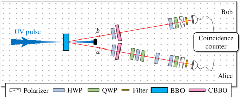
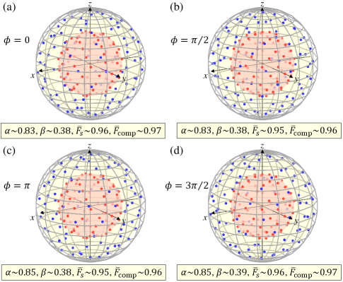
Experiment and results.—In the experiment, we generate photon pairs correlated in the polarization degree of freedom. A schematic diagram of our experimental set-up is shown in Fig. 2. We first implement four different kinds of RSP, denoted as $\mathcal{E}_{\phi}$, while we denote the ideal RSP process as $\mathcal{E}^{(\phi)}_{\text{RSP}}$, which are identified by the choice of single-qubit unitaries, $U=R(\phi)$. The experimental results for the criteria outlined in (i)-(iv), and the concrete comparisons between $\mathcal{E}_{\phi}$, $\mathcal{E}^{(\phi)}_{\text{RSP}}$ and $\mathcal{E}_{c}$ are shown in Fig. 3. The experimental RSPs exhibit quantum process steering and are seen to be close to the target RSP according to the fidelity criteria, which confirms the realizations of nonclassical RSPs.

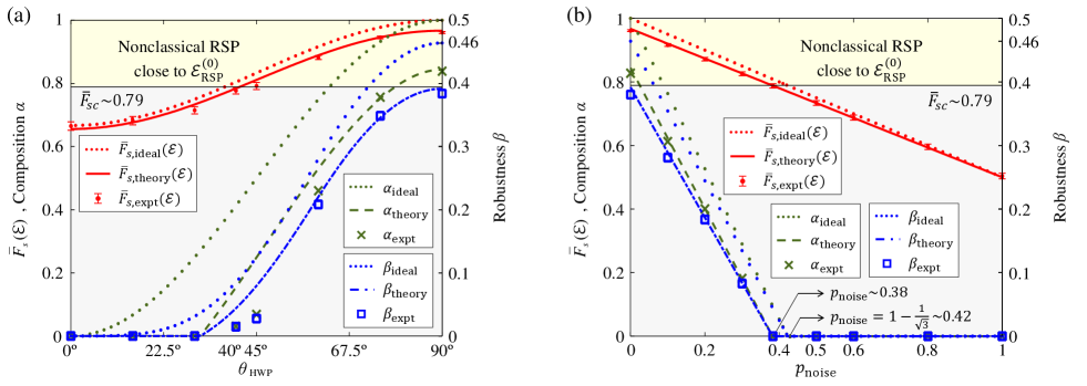
In Fig. 4(a), we demonstrate how the photon walk-off effect affects the process steerability of the resulting RSPs. The walk-off effect describes that the ordinary and the extraordinary photons created via type-II SPDC possess different velocities inside the BBO crystal. Such effect makes generated photon pairs separable and the resulting experimental RSP classical. The walk-off effect can be compensated by a HWP and a CBBO in each mode $a$ and $b$ (see Fig. 2). By varying the compensation of the walk-off of the photons from SPDC, the generated photon pairs can contribute to different process steerabilities. Figure 4(b) shows that experimental process steerability varies with the mixedness of the Werner state $\rho_{W}(p_{\text{noise}})$. To experimentally set the noise weight of $p_{\text{noise}}$, the Werner states were generated by appropriately arranging the measurement durations Lavoie10 ; Amselem09 .

In Fig. 4(a), we show an example where a photon pair with non-zero quantum discord and EPR steerability results in an RSP that does not satisfy the fidelity criteria.The experimental results in Fig. 4(b) illustrate further that $\mathcal{E}_{c}$ can even describe certain RSP processes which rely on quantum discord. They are consistent with the theoretical analysis showing that quantum process steering enables quantum RSP.

We have shown that quantum process steering is the necessary resource that enables RSP to surpass classical dynamical methods of preparing remote states. We experimentally demonstrated this new kind of EPR steering, via several criteria, using different types of polarization-correlated photon states. Our demonstration also shows that other quantum characteristics of polarization-correlated photon pairs, such as quantum discord and standard EPR steering, do not guarantee the existence of nonclassical RSP. Our results outline how to achieve genuine quantum RSP, and are of importance for applications where ruling out any classical mimicries of RSP is necessary. They may provide a useful insight into identifying nonclassical processes for other quantum-information tasks, such as universal one-way quantum computing raussendorf2001 ; briegel2009 ; you2007 ; tanamoto2009 ; wang2010 or quantum communication in quantum networks Chou18 ; Pirker18 .

Acknowledgement.—We acknowledge the fruitful discussions with He Lu. This work was partially supported by the Ministry of Science and Technology, Taiwan, under Grant No. MOST 107-2628-M-006-001-MY4. F.N. is supported in part by: NTT Research, Army Research Office (ARO) (Grant No. W911NF-18-1-0358), Japan Science and Technology Agency (JST) (via the CREST Grant No. JPMJCR1676), Japan Society for the Promotion of Science (JSPS) (via the KAKENHI Grant No. JP20H00134, and the grant JSPS-RFBR Grant No. JPJSBP120194828), and the Grant No. FQXi-IAF19-06 from the Foundational Questions Institute Fund (FQXi), a donor advised fund of the Silicon Valley Community Foundation. N.L. is partially supported by JST PRESTO through Grant No. JPMJPR18GC.

References

- (1) A.K. Pati, Minimum classical bit for remote preparation and measurement of a qubit, Phys. Rev. A 63, 014302 (2000).
- (2) C. H. Bennett, D. P. DiVincenzo, P. W. Shor, J. A. Smolin, B. M. Terhal, and W. K. Wootters, Remote state preparation, Phys. Rev. Lett. 87, 077902 (2001).
- (3) A. Cabello, N-particle N-level singlet states: some properties and applications, Phys. Rev. Lett. 89, 100402 (2002).
- (4) C. H. Bennett, G. Brassard, C. Crépeau, R. Jozsa, A. Peres, and W. K. Wootters, Teleporting an unknown quantum state via dual classical and Einstein-Podolsky-Rosen channels, Phys. Rev. Lett. 70, 1895 (1993).
- (5) S. Pirandola, J. Eisert, C. Weedbrook, A. Furusawa, and S. L. Braunstein, Advances in quantum teleportation, Nat. Photonics 9, 641 (2015).
- (6) E. Jeffrey, N. A. Peters, and P. G. Kwiat, Towards a periodic deterministic source of arbitrary single-photon states, New J. Phys. 6, 100 (2004).
- (7) J. T. Barreiro, T.-C. Wei, and P. G. Kwiat, Remote preparation of single-photon“hybrid” entangled and vector-polarization states, Phys. Rev. Lett. 105, 030407 (2010).
- (8) W. Rosenfeld, S. Berner, J. Volz, M. Weber, and H. Weinfurter, Remote preparation of an atomic quantum memory, Phys. Rev. Lett. 98, 050504 (2007).
- (9) X.-H. Bao, X.-F. Xu, C.-M. Li, Z.-S. Yuan, C.-Y. Lu, and J.-W. Pan, Quantum teleportation between remote atomic ensemble quantum memories, Proc. Natl. Acad. Sci. U.S.A. 109, 20347 (2012).
- (10) H. Ollivier and W. H. Zurek, Quantum discord: A measure of the quantumness of correlations, Phys. Rev. Lett. 88, 017901 (2001).
- (11) W. H. Zurek, Einselection and decoherence from an information theory perspective, Ann. Phys. (Leipzig) 9, 855 (2000).
- (12) L. Henderson and V. Vedral, Classical, quantum and total correlations, J. Phys. A 34, 6899 (2001).
- (13) B. Dakić et al., Quantum discord as resource for remote state preparation, Nat. Phys. 8, 666 (2012).
- (14) B. Dakić, V. Vedral, and Č. Brukner, Necessary and sufficient condition for nonzero quantum discord, Phys. Rev. Lett. 105, 190502 (2010).
- (15) S. Luo and S. Fu, Geometric measure of quantum discord, Phys. Rev. A 82, 034302 (2010).
- (16) N. Killoran, D. N. Biggerstaff, R. Kaltenbaek, K. J. Resch, and N. Lütkenhaus, Derivation and experimental test of fidelity benchmarks for remote preparation of arbitrary qubit states, Phys. Rev. A 81, 012334 (2010).
- (17) H. M. Wiseman, S. J. Jones, and A. C. Doherty, Steering, entanglement, nonlocality, and the Einstein-Podolsky-Rosen paradox, Phys. Rev. Lett. 98, 140402 (2007).
- (18) M. D. Reid, et al., Colloquium: the Einstein-Podolsky-Rosen paradox: from concepts to applications, Rev. Mod. Phys. 81, 1727 (2009).
- (19) M. A. Nielsen and I. L. Chuang, Quantum Computation and Quantum Information (Cambridge Univ. Press, UK, 2000).
- (20) N. Brunner, D. Cavalcanti, S. Pironio, V. Scarani, and S. Wehner, Bell nonlocality, Rev. Mod. Phys. 86, 419 (2014).
- (21) Y.-N. Chen, C.-M. Li, N. Lambert, S.-L. Chen, Y. Ota, G.-Y. Chen, and F. Nori, Temporal steering inequality, Phys. Rev. A 89, 032112 (2014).
- (22) S.-L. Chen, N. Lambert, C.-M. Li, A. Miranowicz, Y.-N. Chen, and F. Nori, Quantifying non-Markovianity with temporal steering, Phys. Rev. Lett. 116, 020503 (2016).
- (23) P. Skrzypczyk, M. Navascués, and D. Cavalcanti, Quantifying Einstein-Podolsky-Rosen steering, Phys. Rev. Lett. 112, 180404 (2014).
- (24) M. Piani and J.Watrous, Necessary and sufficient quantum information characterization of Einstein-Podolsky-Rosen steering, Phys. Rev. Lett. 114, 060404 (2015).
- (25) See Supplemental Material for the comparison between the classical RSP model and the LHS model, and the details of solving optimization problems of the , , and . Moreover, the theoretical model for the compensation of the photon walk-off effect acting on noisy created photon pairs is detailed. Finally, we describe how to measure the discord and EPR steerability of polarization-correlated photon pairs created in our experiments.
- (26) H. F. Hofmann, Complementary classical fidelities as an efficient criterion for the evaluation of experimentally realized quantum operations, Phys. Rev. Lett. 94, 160504 (2005).
- (27) P. G. Kwiat, K. Mattle, H. Weinfurter, A. Zeilinger, A. V. Sergienko, and Y. Shih, New high-intensity source of polarization-entangled photon pairs, Phys. Rev. Lett. 75, 4337 (1995).
- (28) J. Lavoie, R. Kaltenbaek, M. Piani, and K. J. Resch, Experimental bound entanglement in a four-photon state, Phys. Rev. Lett. 105, 130501 (2010).
- (29) E. Amselem and M. Bourennane, Experimental four-qubit bound entanglement, Nat. Phys. 5, 748 (2009).
- (30) R. Raussendorf and H.J. Briegel, A one-way quantum computer, Phys. Rev. Lett. 86, 5188 (2001).
- (31) J. Q. You, X.-B. Wang, T. Tanamoto, and F. Nori, Efficient one-step generation of large cluster states with solid-state circuits, Phys. Rev. A 75, 052319 (2007).
- (32) H. J. Briegel, D. E. Browne, W. Dr, R. Raussendorf, and M. Van den Nest, Measurement-based quantum computation, Nat. Phys. 5, 19 (2009).
- (33) T. Tanamoto, Y. X. Liu, X. Hu, and F. Nori, Efficient quantum circuits for one-way quantum computing, Phys. Rev. Lett. 102, 100501 (2009).
- (34) H. Wang, C.-P. Yang, and F. Nori, Robust and scalable optical one-way quantum computation, Phys. Rev. A 81, 052332 (2010).
- (35) K. S. Chou et al., Deterministic teleportation of a quantum gate between two logical qubits, Nature (London) 561, 368 (2018).
- (36) A. Pirker, J. Wallnöfer, and W. Dür, Modular architectures for quantum networks, New J. Phys. 20, 053054 (2018).
Supplementary Information
I Comparisons between the generalized LHS model and the standard LHS model
The local hidden state (LHS) model Wiseman07 ; Reid09 describes the state of Bob’s qubit conditioned on Alice’s measurement:
- (1) H. M. Wiseman, S. J. Jones, and A. C. Doherty, Steering, entanglement, nonlocality, and the Einstein-Podolsky-Rosen paradox, Phys. Rev. Lett. 98, 140402 (2007).
- (2) M. D. Reid, et al., Colloquium: the Einstein-Podolsky-Rosen paradox: from concepts to applications, Rev. Mod. Phys. 81, 1727 (2009).
- (3) Y.-N. Chen, C.-M. Li, N. Lambert, S.-L. Chen, Y. Ota, G.-Y. Chen, and F. Nori, Temporal steering inequality, Phys. Rev. A 89, 032112 (2014).
- (4) S.-L. Chen, N. Lambert, C.-M. Li, A. Miranowicz, Y.-N. Chen, and F. Nori, Quantifying non-Markovianity with temporal steering, Phys. Rev. Lett. 116, 020503 (2016).
- (5) H. F. Hofmann, Complementary classical fidelities as an efficient criterion for the evaluation of experimentally realized quantum operations, Phys. Rev. Lett. 94, 160504 (2005).
- (6) J.-H. Hsieh, S.-H. Chen, and C.-M. Li, Quantifying quantum-mechanical processes, Sci. Rep. 7, 13588 (2017).
- (7) A. Gilchrist, N. K. Langford, and M. A. Nielsen, Distance measures to compare real and ideal quantum processes, Phys. Rev. A 71, 062310 (2005).
- (8) J. Löfberg, Yalmip: A toolbox for modeling and optimization in MATLAB, in proceedings of the CACSD conference, Taipei, Taiwan, 2004; MATLAB, http://users.isy.liu.se/johanl/yalmip/.
- (9) K. C. Toh, M. J. Todd, and R. H. Ttnc, SDPT3 – a MATLAB software package for semidefinite-quadratic-linear programming, version 4.0., Available: http://www.math.nus.edu.sg/mattohkc/sdpt3.html.
- (10) M. A. Nielsen and I. L. Chuang, Quantum Computation and Quantum Information (Cambridge Univ. Press, UK, 2000).
- (11) I. L. Chuang and M. A. Nielsen, Prescription for experimental determination of the dynamics of a quantum black box, J. Mod. Opt. 44, 2455 (1997).
- (12) P. G. Kwiat, K. Mattle, H. Weinfurter, A. Zeilinger, A. V. Sergienko, and Y. Shih, New high-intensity source of polarization-entangled photon pairs, Phys. Rev. Lett. 75, 4337 (1995).
- (13) D. F. V. James, P. G. Kwiat, W. J. Munro, and A. G. White, Measurements of qubits, Phys. Rev. A 64, 052312 (2001).
- (14) M. H. Rubin, D. N. Klyshko, Y. H. Shih, and A. V. Sergienko, Theory of two-photon entanglement in type-II optical parametric down-conversion, Phys. Rev. A 50, 5122 (1994).
- (15) P. H. Shun, Towards a high quality polarization-entangled multi-photon source, A Thesis Submitted for the Degree of Master of Science, Department of Physics, National University of Singapore (2009).
- (16) S. M. Lee, H. Kim, M. Cha, and H. S. Moon, Polarization-entangled photon-pair source obtained via type-II non-collinear SPDC process with PPKTP crystal, Opt. Express 24, 2941 (2016).
- (17) B. Dakić, V. Vedral, and Č. Brukner, Necessary and sufficient condition for nonzero quantum discord, Phys. Rev. Lett. 105, 190502 (2010).
- (18) P. Skrzypczyk, M. Navascués, and D. Cavalcanti, Quantifying Einstein-Podolsky-Rosen steering, Phys. Rev. Lett. 112, 180404 (2014).