Non-thermalized dynamics of flat-band many-body localization
Abstract
We find that a flat-band fermion system with interactions and without disorders exhibits non-thermalized ergodicity-breaking dynamics, an analog of many-body localization (MBL). In the previous works, we observed flat-band many-body localization (FMBL) in the Creutz ladder model. The origin of FMBL is a compact localized state governed by local integrals of motion (LIOMs), which are to be obtained explicitly. In this work, we clarify the dynamical aspects of FMBL. We first study dynamics of two-particles, and find that the states are not substantially modified by weak interactions, but the periodic time evolution of entanglement entropy emerges as a result of a specific mechanism inherent in the system. On the other hand, as the strength of the interactions is increased, the modification of the states takes place with inducing instability of the LIOMs. Furthermore, many-body dynamics of the system at finite fillings is numerically investigated by time-evolving block decimation (TEBD) method. For a suitable choice of the filling, non-thermal and low entangled dynamics appears. This behavior is a typical example of the disorder-free FMBL.
Introduction.— At present, many-body localization (MBL) is one of the most intensively studied topics, both theoretically and experimentally Nandkishore ; Abanin ; Imbrie . Despite the numerous studies, however, essential properties of MBL and its transition remain an open question. It is now widely accepted that there emerge an extensive number of local conserved quantities in MBL states Nandkishore , which are called local integrals of motion (LIOMs) Serbyn ; Huse , but how the LIOMs behave at transitions out of MBL states is not clear Morningstar ; Vasseur . The LIOMs are the number operator of local bits (-bits), and in most of the studies on the LIOMs given so far, -bits are constructed, e.g., from single-particles states of Anderson localization. Therefore, they are numerically obtained Bera ; Imbrie1 ; Rademarker1 ; You1 ; Pekker1 ; Brien1 ; Wahl1 ; Pal1 ; Tomasi ; Peng ; Nicolas and depend on the random potential originating Anderson localization. Study on systems with explicit form of -bits is certainly desired and welcome.
In the previous works KOI2020 ; OKI2020 , we investigated Creutz ladder model Creutz1999 ; Bermudez ; Junemann ; Tovmasyan ; Sun ; Barbarino_2019 with interactions, in which all single particle spectra are flat, for motivation finding MBL-like behaviors. In fact by using exact diagonalization, this expectation was verified KOI2020 ; Roy . General discussion of the presence of flat-band MBL (FMBL) has been reported Danieli_1 . The origin of localization in that system comes from compact localized states Leykam ; Zurita ; Zhou ; kuno2020 , which can be regarded as -bits from the view point of MBL. In the single-particle level, the number operator of the compact-localized state is LIOMs. All energy eigenstates in the model have a finite support and the energy level is degenerate in the non-interacting limit. Even in the presence of interactions, one may expect that the effects of the single-particle LIOMs remain and they make the system localized KOI2020 . We call this phenomenon FMBL. Signature of FMBL has been reported not only for the Creutz ladder but also other flat-band models Roy ; Zurita ; Paul ; Daumann ; Tilleke ; Khare . However, its dynamical properties have not been clarified so far. In particular, dynamical entanglement properties of FMBL is not completely understood, though some studies on it have been given, e.g., from the perspective on the Aharanov-Bohm caging vidal0 ; vidal1 with interactions Liberto ; Danieli1 ; Danieli2 ; KMH2020 . In this Letter, we clarify the dynamics of FMBL for Creutz-ladder fermions with the explicit LIOMs by observing the quantities employed in studying the conventional MBL states Nandkishore ; Abanin ; Imbrie .
First, we study two-particle dynamics to elucidate the entanglement properties of the system since the -bit picture is significantly clear there. With interactions, entanglement entropy () is produced, whose behavior gives an insight into the many-body dynamics of FMBL. We then investigate many-body states at finite fillings. We find a FMBL state that exhibits non-thermalizing behavior, i.e., memory of an initial state is preserved, and also a nontrivial slow growth of appears, which is not logarithmic growth as in the conventional MBL state Bardarson . The stability of non-thermal dynamics depends on the particle filling. We find that it is determined by robustness of the -bit picture.
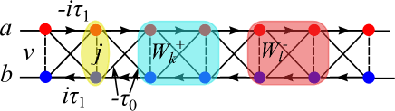
Model.— Target model is the Creutz ladder system with Hamiltonian given as follows,
| (1) | |||||
where and are fermion annihilation operators at site , and and are intra-chain and inter-chain hopping amplitudes, respectively. The corresponding system has been experimentally realized Shin2020 . For , the system has two bands, which are strictly flat, and the perfect localization is realized. The Hamiltonian (1) is written as a summation of LIOMs such as with the -bits ,
| (2) | |||||
| (3) | |||||
It is readily verified In what follows, we set . Then, all single-particle eigenstates are given as with energy . A single localized particle exhibits the Aharanov-Bohm caging vidal0 ; vidal1 around the plaquette . The particle does not spread out through the system and oscillates around the initial site. As a result, exact localized dynamics appears in a single particle level.
From in Eq. (2), operators are nothing but LIOMs, which play an important role in study on localization. Besides in (2), the system Hamiltonian can have an inter-leg hopping term. The effect of it is studied in Supp in order to investigate properties of extended states.
Two-particle system.— Let us first consider two-particle system to investigate effects of the interactions such as , where and . Study on the two-particle system gives an insight on dynamics of many-body states that we consider later on. The target system is given by with the unit of energy . We numerically study . The entanglement entropy is defined as the von-Neumann entanglement entropy for a reduced density matrix for a subsystem, , where is a reduced density matrix, is a many-body eigenstate and system is divided into A and B subsystem. We also calculate expectation values of particle density and LIOMs, during time evolution. As well as the above quantities, we introduce the fourth-order moment of LIOMs, , where . The fourth-order moment of LIOMs quantifies the stability of the LIOMs in states remark1 . In later investigation, its measure indicates local enhancement of -bit, which is an interesting phenomenon.
As in Ref. Serbyn2012_2 , we first consider a two-particle system in which each particle state consists of a superposition of two states such as . This consideration of the two-particle states gives very important insight on FMBL. In the practical calculation, we put the distance between two states . For , effects of interactions do not work. Density matrix and of the -subsystem are defined as usual by taking trace of the -subsystem remark2 .
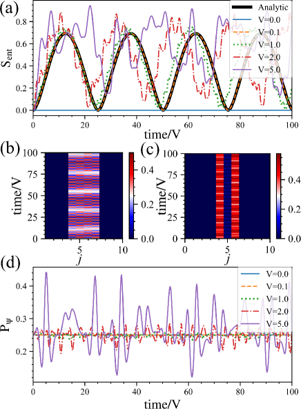
In Fig. 1 (a), we show observation of time evolution of for various values of Quspin . Initial state is , and is obtained by integrating out quantum degrees of freedom on sites . The initial two-particles start to spread out by Aharanov-Bohm caging and then, the particles interact with each other via the nearest-neighbor components of .
The calculations of exhibit very interesting behavior. For small , oscillates periodically, and the period is almost the same for ’s smaller than unity. We also show the analytical solution of the dynamics of (See Supp ). The numerical results for small are in good agreement with the analytical result. One may think that this behavior comes from a similar effect to that in the well-separated two-particle system studied in Ref. Serbyn2012_2 . However, this is not the case. By assuming that the states are not modified by the weak interactions, let us focus on the four states, and In the usual case Serbyn2012_2 , the interaction energy between particles located at sites and in the -particle representation gerenates , which exhibits an oscillating behavior in time. In the present case however, the states and are strictly degenerate. Furthermore, the interaction cannot be expressed solely in terms of the LIOMs, ’s, and there exist terms such as , etc. In fact, it is easily verified . Therefore, the mixing between and must be suitably taken into account by considering linear combinations to study the time evolution of the states, although the above non-LIOM terms can be neglected in certain cases Tomasi ; Nicolas . The above properties are very characteristic ones and essential for the time evolution in the flat-band system. We have also verified that other mixing between states such as and does not plays a substantial role in the time evolution of . For , consideration within the space is legitimate as modification of states is negligible, and as a result, the values of the peaks of in Fig. 1 (a) is very close to the theoretical value, . Our estimated period of oscillation is , which is also very close to the results in Fig. 1 (a).
On the other hand for and , displays rather complicated behavior and it becomes larger than in certain temporal periods. This indicates that a modification of eigenstates by the interactions takes place, and states other than emerge. In order to verify the above observation, we display the time evolution of the particle density and in Figs. 1 (b) and (c) for . As expected, the particle densities exhibit rather strong oscillating behavior. Similar behavior is observed for . Furthermore, the calculation of the fourth-order moment of LIOMs in Fig. 1 (d) is quite instructive. In the initial state, for and otherwise zero at . Therefore . The calculation of the the fourth-order moment of LIOMs indicates that the initial particle state is stable for but is strongly modified by the interactions for under the time evolution. The oscillation of and at peaks mean that not only destruction of -bit but also certain local enhancement of -bit takes place under the time evolution. At present, if this phenomenon is peculiar properties of the present model is not known. This is an interesting future problem. Anyway, modification of states is observed, as the interactions dominate the energy gap between the two flat bands for . This phenomenon has not been observed in the past.
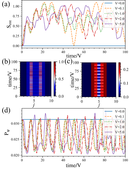
As the second case, we prepare an initial state such as, , where the distance of the initial two-particles is three site, . This configuration is closely related with a many-body state studied later on. The initial two-particles again spread first by Aharanov-Bohm caging and then, the particles interact with each other by . of the two-particles for various ’s is plotted in Fig. 2 (a) remark2 . While the particles are not entangled in the absence of interactions, exhibits clear oscillation for finite and no saturation. For , exhibits an oscillation with multiple periods. This behavior is different from that of the first case, but it stems from the fact that the initial state is a superposition of eigenstates of the flat Hamiltonian, , (See Supp ). Therefore, various resonant states emerge in the time evolution similar to the first case. On the other hand for and , shows rather complicated behavior. This indicates a modification of eigenstates by the interactions. However, the values of the peaks of are in between and .
As the density profile in Fig. 2 (b) shows, two-particles do not spread out from the sites for . The LIOMs distribution in Fig. 2 (c) for has finite value in dynamics, while it oscillates nontrivially. Thus, the -bit picture survives even for the interactions. We have verified a similar behavior for .
The calculation of the fourth-order moment of LIOMs in Fig. 2 (d) shows how the LIOM picture changes in the time evolution. The fourth-order moment of LIOMs for finite ’s fluctuates but revivals to the initial value, . This indicates that the initial LIOM picture governs the dynamics and keeps the particles localized for a long period. For a homogeneous state at finite fillings, it is plausible to expect that the repulsions between particles suppresses the density fluctuations and enhances localization, and then the -bit picture and LIOMs work effectively to describe localized states. We shall verify this expectation in the following.
Finite-density states.— The study of the two-particle systems revealed a very interesting phenomenon, that is, develops substantially under time evolution, whereas the revival of the LIOMs takes place at the same time. We expect that this phenomenon comes from the fact that the energy eigenstates in the non-interacting system are the same or quite similar even for and , and then, mixings of these states occur quite easily. From this consideration, we expect that some specific localization behavior emerges in the system at finite fillings. Properties of configurations may strongly depend on the filling factor.
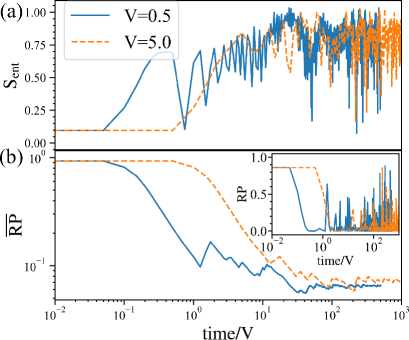
With this expectation, we investigate many-particle dynamics by employing the TEBD method in TeNPy package TenPy . The validity of the TEBD method is examined Supp and sufficiently careful manipulations are given. In what follows, we set open boundary condition. We first consider an initial state with particle filling , and calculate for the subsystem of the left half of the ladder and return probability . In this particle filling, all particles initially start Aharanov-Bohm caging, and after that the particles interact with each other. This behavior is similar to the two-particle systems studied in the above. The results obtained by TEBD are displayed in Fig. 3. For early times (), increases and then saturates. The saturation value is independent of the strength of the repulsion, , and comparable to the maximum of of the two-particle dynamics in Fig. 2 (a), which is smaller than that of a conventional thermal (extended) many-body states. The return probability in Fig. 3 (b) also shows an interesting behavior, that is, the PR clearly oscillates even for a long-time, and this character is also independent of the value of . The memory of the initial state is conserved. We expect that the origin of this phenomenon is the remnants of LIOM picture in the flat-band system, i.e., the -bits survive in the presence of the interactions by the mechanism that we observed for the two-particle system. From the results of and return probability, the system is not thermalized and this indicates ergodicity breaking dynamics, expected by our small system-size calculations in KOI2020 . The above characters are analog of the dynamical behavior of the conventional MBL Huse , but there is a difference, i.e., the does not exhibit a logarithmic increase. We expect that this is a signature of the localization mechanism in the flat-band system, which works efficiently for the homogeneous states. In addition, it should be commented that in Rydberg atom, it has been observed that the revival dynamics occurs for a long time when the initial state is taken as Neel state Bernien . There is a gauge-theoretical interpretation of this phenomenon Smith1 ; Smith2 ; PRD ; Surace . It is just a string inversion mechanism. We observe similarity between the LIOMs and gauge-invariance constraint.
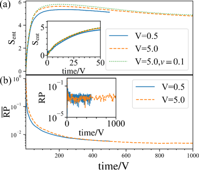
An initial state with particle filling , is also studied. The particles in this case interact with each other more strongly than the case of the filling (See Supp ). The time evolution of this case, shown in Fig. 4, seems quite different from that of the -filling case in Fig. 3. It indicates that the -bit picture is broken as a result of substantial modification of states. The filling is an extended state. Actually, the value of of the -filling flat band with interactions saturates to the same value of the band bending case constructed by inclusion of a vertical hopping, .
Conclusion.—
We clarified dynamical aspect, especially entanglement property, of the FMBL in the Creutz ladder model
with interactions.
The LIOM obtained by -bit (compact localized state) plays a major role in the appearance of the FMBL.
Starting with studying the fate of the Aharanov-Bohm caging with interactions for the two-particle dynamics,
we investigated many-body dynamics by using the TEBD.
The presence of the FMBL is determined by the balance of particle filling and the range of inter-particle interactions.
For a suitable choice of particle filling,
the many-body dynamics with interactions exhibits non-thermalized behavior with low-entanglement growth and finite return probability.
The -bit picture and LIOMs in the flat-band system survive there.
This work was supported by the Grant-in-Aid for JSPS Fellows (No.17J00486).
References
- (1) R. Nandkishore, and D. A. Huse, Annual Review of Condensed Matter Physics 6, 15 (2015).
- (2) D. A. Abanin, E. Altman, I. Bloch, and M. Serbyn, Rev. Mod. Phys. 91, 021001 (2019).
- (3) J. Z. Imbrie, V. Ros, and A. Scardicchio, Annalen der Physik 529, 1600278 (2017).
- (4) M. Serbyn, Z. Papić , and D. A. Abanin, Phys. Rev. Lett. 111, 127201 (2013).
- (5) D. A. Huse, R. Nandkishore, and V. Oganesyan, Phys. Rev. B 90, 174202 (2014).
- (6) A. Morningstar and D. A. Huse, Phys. Rev. B 99, 224205 (2019).
- (7) P. T. Dumitrescu, A. Goremykina, S. A. Parameswaran, M. Serbyn, and R. Vasseur, Phys. Rev. B 99, 094205 (2019).
- (8) S. Bera, H. Schomerus, F. Heidrich-Meisner and J. H. Bardarson, Phys. Rev. Lett. 115, 046603 (2015).
- (9) J. Z. Imbrie, J. Sat. Phys 163, 998 (2016).
- (10) L. Rademarker and M. Ortuño, Phys. Rev. Lett. 116, 010404 (2016).
- (11) Y. Z. You, X. L. Qi, and C. Xu, Phys. Rev. B 93, 104205 (2016).
- (12) D. Pekker, B. K. Clark, V. Oganesyan, and G. Rafael, Phys. Rev. Lett. 119, 075701 (2017).
- (13) T. E. O’Brien, D. A. Abanin, G. Vidal, and Z. Papić, Phys. Rev. B 94, 144208 (2016).
- (14) T. B. Wahl, A. Pal, and S. H. Simon, Phys. Rev. X 7, 021018 (2017).
- (15) A. K. Kulshreshtha, A. Pal,T. B. Wahl, and S. H. Simon, Phys. Rev. B 99, 104201 (2019).
- (16) G. De Tomasi, F. Pollmann, and M. Heyl, Pys. Rev. B 99, 241114(R) (2019).
- (17) P. Peng, Z. Li, H. Yan, K.X. Wei, and P. Cappellaro, Phys. Rev B 100, 214203 (2019).
- (18) N. Laflorencie, G. Lemarié, and N. Macé, Phys. Rev. Research 2, 042033(R) (2020).
- (19) Y. Kuno, T. Orito, and I. Ichinose, New J. Phys. 22, 013032 (2020).
- (20) T. Orito, Y. Kuno, and I. Ichinose, Phys. Rev. B 101, 224308 (2020).
- (21) M. Creutz, Phys. Rev. Lett. 83, 2636 (1999).
- (22) A. Bermudez, D. Patanè, L. Amico, and M. A. Martin-Delgado, Phys. Rev. Lett. 102, 135702 (2009).
- (23) J. Jünemann, A. Piga, L. Amico, S.-J. Ran, M. Lewenstein, M. Rizzi, and A. Bermudez, Phys. Rev. X 7, 031057 (2017).
- (24) S. Tovmasyan, S. Peotta, P. Törmä, and S. D. Huber, Phys. Rev. B 94, 245149 (2016).
- (25) N. Sun, and L.-K. Lim, Phys. Rev. B 96, 035139 (2017).
- (26) S. Barbarino, D. Rossini, M. Rizzi, M. Fazio,G. E. Santoro and M. Dalmonte, New J. Phys. 21, 043048 (2019).
- (27) N. Roy, A. Ramachandran, and A. Sharma, arXiv: 1912.09951 (2019).
- (28) C. Danieli, A. Andreanov, and S. Flach, Phys. Rev. B 102, 041116 (2020).
- (29) D. Leykam, A. Andreanov, and S. Flach, Adv. Phys. X 3, 1473052 (2018).
- (30) J. Zurita, C. E. Creffield, and G. Platero, Advanced Quantum Technologies 3, 1900105 (2020).
- (31) L. Zhou, and Q. Du , Phys. Rev. A 101, 033607 (2020).
- (32) Y. Kuno, Phys. Rev. B 101, 184112 (2020).
- (33) P. A. McClarty, M. Haque, A. Sen, and J. Richter, Phys. Rev. B 102, 224303 (2020).
- (34) M. Daumann, R. Steinigeweg, T. Dahm, arXiv: 2009.09705 (2020).
- (35) S. Tilleke, M. Daumann, and T. Dahm, Zeitschrift für Naturforschung A 75, 393 (2020).
- (36) R. Khare, and S. Choudhury, J. Phys. B 54, 015301 (2021).
- (37) J. Vidal, R. Mosseri, and B. Douçot, Phys. Rev. Lett. 81, 5888 (1998).
- (38) J. Vidal, B. Douçot, R. Mosseri, and P. Butaud, Phys. Rev. Lett. 85, 3906 (2000).
- (39) M. Di Liberto, S. Mukherjee, and N. Goldman, Phys. Rev. A 100, 043829 (2019).
- (40) C. Danieli, A. Andreanov, T. Mithun, and S. Flach, arXiv: 2004.11871 (2020).
- (41) C. Danieli, A. Andreanov, T. Mithun, and S. Flach, arXiv: 2004.11880 (2020).
- (42) Y. Kuno, T. Mizoguchi, Y. Hatsugai, Phys. Rev. A 102, 063325 (2020).
- (43) J. H. Bardarson, F. Pollmann, and J. E. Moore, Phys. Rev. Lett. 109, 017202 (2012).
- (44) J. H. Kang, J. H. Han, and Y. Shin, New J. Phys. 22, 013023 (2020).
- (45) See Supplemental Material; (i) One-particle system and its dynamics, (ii) Analytical solution of dynamics of entanglement entropy for small and (iii) Validity and technical comments for numerical TEBD simulations.
- (46) In observing dynamics of the system the fourth-order moment of LIOMs is efficient to estimate the deviation from the LIOM picture of the initial state.
- (47) M. Serbyn, Z. Papić, D. A. Abanin, Phys. Rev. Lett. 110, 260601 (2013).
- (48) -subsystem is the subsystem of the left half of the ladder and -subsystem is of the right.
- (49) We employed the Quspin solver: P. Weinberg and M. Bukov, SciPost Phys. 7, 20 (2019); 2, 003 (2017).
- (50) J. Hauschild and F. Pollmann, SciPost Phys. Lect. Notes 5 (2018).
- (51) H. Bernien, S. Schwartz, A. Keesling, H. Levine, A. Omran, H.Pichler, S. Choi, A. S. Zibrov, M. Endres, M. Greiner et al., Nature (London) 551, 579 (2017).
- (52) A. Smith, J. Knolle, D. L. Kovrizhin, and R. Moessner, Phys. Rev. Lett. 118, 266601 (2017).
- (53) A. Smith, J. Knolle, R. Moessner, and D. L. Kovrizhin, Phys. Rev. Lett. 119, 176601 (2017).
- (54) Y Kuno, S. Sakane, K. Kasamatsu, I Ichinose, and T. Matsui, Phys. Rev. D 95, 094507 (2017).
- (55) F. M. Surace, P. P. Mazza, G. Giudici, A. Lerose, A. Gambassi, and M. Dalmonte, Phys. Rev. X 10, 021041 (2020).
Supplemental Material
.1 One-particle system and its dynamics
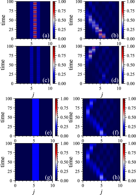
We study dynamical behaviors of single-particle states for in (2) in the main text. The schematic figure of the model is given in Fig. 5. The dynamics is obtained by the exact diagonalization Quspin . Here, besides in (2) in the main text, we also add inter-leg hopping, defined by . This hopping makes the band dispersive and destroys the localization properties. Here, we investigate the effects of . For the genuine system with Eq. (2) in the main text, are perfect constants of motion, whereas and break the conservation of the LIOMs.
As the initial state, the single-particle state such as is employed. We study the time evolution of the particle densities and LIOMs, . For the system in Eq. (2), the a/b-particle densities during time evolution are quite stable as shown in Figs. 6 (a) and (c), and the LIOM remains constant as shown in Figs. 6 (e) and (g). These results are just Aharanov-Bohm caging vidal0 ; vidal1 . On the other hand, once one switches on or sets , it breaks the flat-band structure, and induces instability of the LIOMs. As shown in Figs. 6 (b), (d), and (f), the a- and b- particle densities spread over the whole system, and the LIOMs are not conserved. However, it is interesting and instructive to see that region with the significant expectation values of the LIOMs, , moves without breaking its shape and bounces at the boundary.
.2 Analytical solution of dynamical entanglement entropy for small
In Fig.1 in the main text, we consider the two-particle dynamics with the initial state; . Analytical solution of the dynamical entanglement entropy () for small can be obtained by applying the simple perturbation theory for degenerate states. Here, we consider the flat-band case.
The initial state is a superposition of the two-particle states, , , and . For , the states and are degenerate with the vanishing energy. Thus, to obtain the dynamics , we need to calculate the two-particle wave function at time . To this end, we calculate perturbated energies and the corresponding perturbated eigenstates for the two-particle states. For the Hamiltonian ( is non-perturbative and is perturbative), the first order perturbation theory gives the following two-particle approximated non-degenerate eigenstates straightfowardly,
| (4) |
Here, () are perturbated eigenstates from the states, , , and .
By using the above eigenstates, we get the time-evolved state as follows,
| (5) | |||||
From this time-evolved wave function, the partial density matrix is obtained as follows by tracing out the right half of the system,
| (6) |
Therefore, the time evolution of defined by is given by
| (7) | |||||
This solution exhibits an oscillation with the period , which is plotted in Fig. 1 (a) in the main text.
.3 Validity and technical comments on numerical TEBD simulations
For many-body dynamics, we employ the time-evolving block decimation (TEBD) method by using TeNPy package TenPy . By comparing the method to the exact diagonalization of Quspin package Quspin , we verify the validity of the TEBD method for the flat-band system in the main text.
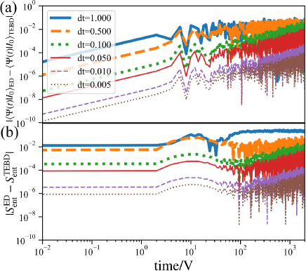
We consider the system with and . The system size is (20 sites) and employ the open boundary condition. We set an initial state, , and measure the return probability and the entanglement entropy, , for the subsystem of the left half of the ladder as defined in the main text. Here, as a technical aspect, it should be noted that for the TEBD calculation, we add very small band bending by including the cross hopping term with to avoid the zero-energy effects in exact flat band situation, but such a small modification has little effects on the dynamics of the physical quantities of interest. We show this fact by comparing with the exact diagonalization, which does not include such a band bending.
Except for the modification in the TEBD method, we calculate the dynamics by the TEBD and exact diagonalization in the same condition. Figure 7 (a) and (b) are the comparison between both calculations for various intervals of time step, . For smaller , Both differences for the return probability and decrease. For the difference of the return probability, the value is almost below for within our target time interval . The error does not affect our focusing physics. For the cauclulations of , the same order of accuracy is verified as shown in Fig. 7 (b). The value of the difference is almost below for within our target time interval . Therefore, the error also does not affect our focusing physics. From the above studies on the accuracy of the numerical methods, for our TEBD calculations in the main text, we set and included small band bending by .