Non-Riemannian Volume Elements Dynamically Generate Inflation

The theoretical framework based on the concept of “inflation” in the study of the evolution of the early Universe provides an attractive solution explaining the “puzzles” of Big-Bang cosmology (the horizon problem, the flatness problem, the magnetic monople problem, etc. [1]-[5]. Likewise it is an important instrumentarium for treatment of primordial density perturbations [6, 7]. For some recent detailed accounts, see Refs.[8]-[12].

On the other hand, in a parallel development another groundbreaking concept emerged in the last decade or so about the intrinsic necessity to modify (extend) gravity theories beyond the scope of standard Einstein’s general relativity with the main motivation to overcome the limitations of the latter coming from: (i) Cosmology – for solving the problems of dark energy and dark matter and explaining the large scale structure of the Universe [13, 14]; (ii) Quantum field theory in curved spacetime – due to renormalization of ultraviolet divergences in higher loops [15]; (iii) Modern string theory – due to the natural appearance of higher-order curvature invariants and scalar-tensor couplings in low-energy effective field theories [16].

Various classes of modified gravity theories have been employed to construct viable inflationary models: $f(R)$-gravity; scalar-tensor gravity; Gauss-Bonnet gravity (see Refs.[17]-[21] for a detailed accounts); recently also based on non-local gravity (Ref.[22] and references therein) or based on brane-world scenarios (Ref.[23] and references therein). The first early successful cosmological model based on the extended $f(R)=R+R^{2}$-gravity is the classical Starobinsky potential [1].

A further specific broad class of actively developed modified (extended) gravitational theories is based on the formalism of non-Riemannian spacetime volume elements (originally proposed in Refs.[24]-[28]; see Refs.[29, 30] for a systematic geometric formulation). This formalism was used as a basis for constructing a series of extended gravity-matter models describing unified dark energy and dark matter scenario [31, 32], quintessential cosmological models with gravity-assisted and inflaton-assisted dynamical suppression (in the “early” universe) or dynamical generation (in the post-inflationary universe) of electroweak spontaneous symmetry breaking and charge confinement [33]-[35], as well as a novel mechanism for dynamical supersymmetric Brout-Englert-Higgs effect in supergravity [29].

In what follows we will describe in some detail the construction of a viable cosmological inflationary model starting from a modified pure gravity involving several independent non-Riemannian volume elements and without any a priori coupling to matter fields.

Let us briefly recall the essence of the non-Riemannian volume-form formalism (cf. Ref.[36]).

In integrals over differentiable manifolds (not necessarily Riemannian one, so no metric is needed) volume-forms are given by nonsingular maximal rank differential forms $\omega$:

$$\int_{{\mathcal{M}}}\omega\bigl{(}\ldots\bigr{)}=\int_{{\mathcal{M}}}dx^{D}\,\Omega\bigl{(}\ldots\bigr{)}\;\;,\;\;\omega=\frac{1}{D!}\omega_{\mu_{1}\ldots\mu_{D}}dx^{\mu_{1}}\wedge\ldots\wedge dx^{\mu_{D}}\;,$$

(1)

where $\omega_{\mu_{1}\ldots\mu_{D}}=-\varepsilon_{\mu_{1}\ldots\mu_{D}}\Omega$ and $\Omega$ is the volume element density (our conventions for the totally anti-symmetric symbols are $\varepsilon^{01\ldots D-1}=1\;,\;\varepsilon_{01\ldots D-1}=-1$).

In Riemannian $D$-dimensional spacetime manifolds a standard generally-covariant volume-form is defined through the “D-bein” (frame-bundle) canonical one-forms $e^{A}=e^{A}_{\mu}dx^{\mu}$ ($A=0,\ldots,D-1$):

$$\omega=e^{0}\wedge\ldots\wedge e^{D-1}=\det\|e^{A}_{\mu}\|\,dx^{\mu_{1}}\wedge\ldots\wedge dx^{\mu_{D}}\;,$$

(2)

where the standard Riemannian volume element density reads $\Omega=\det\|e^{A}_{\mu}\|=\sqrt{-\det\|g_{\mu\nu}\|}\equiv\sqrt{-g}$.

To construct modified gravitational theories as alternatives to ordinary standard theories in Einstein’s general relativity, instead of $\sqrt{-g}$ we can employ one or more alternative non-Riemannian volume element(s) as in (1) given by non-singular exact $D$-forms $\omega=dA$, where: $A=\frac{1}{(D-1)!}A_{\mu_{1}\ldots\mu_{D-1}}dx^{\mu_{1}}\wedge\ldots\wedge dx^{\mu_{-1}}$ and the corresponding volume element density reads:

$$\Omega\equiv\Phi(A)=\frac{1}{(D-1)!}\varepsilon^{\mu_{1}\ldots\mu_{D}}\,\partial_{\mu_{1}}A_{\mu_{2}\ldots\mu_{D}}\;.$$

(3)

Thus, non-Riemannian volume element densities $\Phi(A)$ are defined in terms of the (scalar density of the) dual field-strength of auxiliary rank $D-1$ tensor gauge fields $A_{\mu_{1}\ldots\mu_{D-1}}$.

As an important remark, let us note that in the first-order (Palatini) formalism ($g_{\mu\nu}$ and $\Gamma_{\mu\nu}^{\lambda}$ a priori independent), the auxiliary tensor gauge fields $A_{\mu_{1}\ldots\mu_{D-1}}$ turn out to be (almost) pure-gauge – no propagating field degrees of freedom except for few discrete degrees of freedom with conserved canonical momenta appearing as arbitrary integration constants. See Refs.[30]-[33] (appendices A) for a systematic proof of the latter fact using the standard canonical Hamiltonian treatment of systems with gauge symmetries, i.e., systems with first-class Hamiltonian constraints a’la Dirac [37, 38].

However, in the second-order (metric) formalism (where $\Gamma_{\mu\nu}^{\lambda}$ is the usual Levi-Civita connection of the metric $g_{\mu\nu}$) the first non-Riemannian volume form $\Phi(A)$, replacing $\sqrt{-g}$ in the modified Einstein-Hilbert part of the action:

$$S=\int d^{4}x\Phi(A)R+\ldots\;,$$

(4)

is not any more pure-gauge. The reason is that in the action (4) the scalar curvature $R$ (in the metric formalism) containes second-order (time) derivatives (the latter amount to a total derivative in the ordinary case $S=\int d^{4}x\sqrt{-g}R+\ldots$).

So defining $\chi_{1}\equiv\Phi(A)/\sqrt{-g}$, the latter field becomes physical degree of freedom as seen from the equations of motion resulting from varying (4) w.r.t. $g^{\mu\nu}$:

$$R_{\mu\nu}+\frac{1}{\chi_{1}}\bigl{(}g_{\mu\nu}\Box\chi_{1}-\nabla_{\mu}\nabla_{\nu}\chi_{1}\bigr{)}+\ldots=0$$

(5)

Let us now consider the following simple modified gravity model without any couplings to matter fields (we will use “Planck units” $16\pi G_{N}=1$):

$$S=\int d^{4}x\Bigl{\{}\Phi_{1}(A)\Bigl{[}R-2\Lambda_{0}\frac{\Phi_{1}(A)}{\sqrt{-g}}\Bigr{]}+\Phi_{2}(B)\frac{\Phi_{0}(C)}{\sqrt{-g}}\Bigr{\}}\;.$$

(6)

Here $R$ is the scalar curvature in the metric formalism and:

	$\displaystyle\Phi_{1}(A)\equiv\frac{1}{3!}\varepsilon^{\mu\nu\kappa\lambda}\partial_{\mu}A_{\nu\kappa\lambda}\;,\;\Phi_{2}(B)\equiv\frac{1}{3!}\varepsilon^{\mu\nu\kappa\lambda}\partial_{\mu}B_{\nu\kappa\lambda}\;,$
	$\displaystyle\Phi_{0}(C)\equiv\frac{1}{3!}\varepsilon^{\mu\nu\kappa\lambda}\partial_{\mu}C_{\nu\kappa\lambda}\;,\phantom{aaaaaa}$		(7)

denote three different independent non-Riemannian volume element denisties as in (3) for $D=4$. $\Lambda_{0}$ is dimensionful parameter which will turn out in what follows to play the role of an inflationary scale.

It is important to stress that the form of the action (6) is uniquely specified by the requirement about global Weyl-scale invariance under:

$\displaystyle g_{\mu\nu}\to\lambda g_{\mu\nu}\;,\;A_{\mu\nu\kappa}\to\lambda A_{\mu\nu\kappa}\;,\;B_{\mu\nu\kappa}\to\lambda^{2}B_{\mu\nu\kappa}\;,\;C_{\mu\nu\kappa}\to C_{\mu\nu\kappa}\;.$

(8)

where $\lambda={\rm const}$. Its importance within the context of non-Riemannian volume element formalism has been originally stressed in [26].

The equations of motion from the action (6) w.r.t. the auxiliary gauge fields $A_{\mu\nu\lambda},\,B_{\mu\nu\lambda}\,,C_{\mu\nu\lambda}$ defining the non-Riemannian volume elements (7) yield, respectively:

	$\displaystyle R-4\Lambda_{0}\frac{\Phi_{1}(A)}{\sqrt{-g}}=-M_{1}\equiv{\rm const}\;,$		(9)
	$\displaystyle\frac{\Phi_{0}(C)}{\sqrt{-g}}=-M_{2}\equiv{\rm const}\;\;,\;\;\frac{\Phi_{2}(B)}{\sqrt{-g}}=\chi_{2}\equiv{\rm const}\;.$		(10)

Here $M_{1},M_{2}$ and $\chi_{2}$ are (dimensionful and dimensionless, respectively) free integration constants; $M_{1},M_{2}$ indicate spontaneous breaking of global Weyl symmetry (8).

Also, it is important to observe that, since the scalar curvature $R$ contains terms with second-order time derivatives on $g_{\mu\nu}$, Eq.(9) is a genuine dynamical equation of motion and not a constraint.

The equations of motion w.r.t. $g_{\mu\nu}$ from (6) read:

$$R_{\mu\nu}-\Lambda_{0}\chi_{1}\,g_{\mu\nu}+\frac{1}{\chi_{1}}\bigl{(}g_{\mu\nu}\Box{\chi_{1}}-\nabla_{\mu}\nabla_{\nu}\chi_{1}\Bigr{)}-\frac{\chi_{2}M_{2}}{\chi_{1}}g_{\mu\nu}=0\;,$$

(11)

with $\chi_{1}\equiv\Phi(A)/\sqrt{-g}$. Taking the trace of (11):

$$3\frac{\Box\chi_{1}}{\chi_{1}}-\frac{4\chi_{2}M_{2}}{\chi_{1}}-M_{1}=0$$

(12)

yields a dynamical equation of motion for the composite scalar field $\chi_{1}$.

We now transform Eqs.(11) and (12) to the physical Einstein frame via the conformal transformation ${\bar{g}}_{\mu\nu}=\chi_{1}g_{\mu\nu}$, upon using the well-known (cf. Ref.[39]) conformal transformation formulas (bars indicate magnitudes in the ${\bar{g}}_{\mu\nu}$-frame):

	$\displaystyle R_{\mu\nu}(g)=R_{\mu\nu}(\bar{g})-3\frac{{\bar{g}}_{\mu\nu}}{\chi_{1}}{\bar{g}}^{\kappa\lambda}\partial_{\kappa}\chi_{1}^{1/2}\partial_{\lambda}\chi_{1}^{1/2}$
	$\displaystyle+\chi_{1}^{-1/2}\bigl{(}{\bar{\nabla}}_{\mu}{\bar{\nabla}}_{\nu}\chi_{1}^{1/2}+{\bar{g}}_{\mu\nu}{\bar{\Box}}\chi_{1}^{1/2}\bigr{)}\;,$		(13)
	$\displaystyle\Box\chi_{1}=\chi_{1}\Bigl{(}{\bar{\Box}}\chi_{1}-2{\bar{g}}^{\mu\nu}\frac{\partial_{\mu}\chi_{1}^{1/2}\partial_{\nu}\chi_{1}}{\chi_{1}^{1/2}}\Bigr{)}\;.$		(14)

Hereby the transformed equations acquire the standard form of Einstein equations w.r.t. the new “Einstein-frame” metric ${\bar{g}}_{\mu\nu}$:

	$\displaystyle R_{\mu\nu}(\bar{g})-\frac{1}{2}{\bar{g}}_{\mu\nu}R(\bar{g})=\frac{1}{2}\Bigl{[}\partial_{\mu}u\partial_{\nu}u-{\bar{g}}_{\mu\nu}\bigl{(}\frac{1}{2}{\bar{g}}^{\kappa\lambda}\partial_{\kappa}u\partial_{\lambda}u+U_{\rm eff}(u)\bigr{)}\Bigr{]}\;,$		(15)
	$\displaystyle{\bar{\Box}}u+\frac{{\partial{U_{\rm eff}}}}{{\partial{u}}}=0\;,$		(16)

where we have redefined

$$\Phi_{1}(A)/\sqrt{-g}\equiv\chi_{1}=\exp{\bigl{(}u/\sqrt{3}\bigr{)}}$$

(17)

in order to obtain a canonically normalized kinetic term for the scalar field $u$, and where we have obtained a dynamically generated effective scalar potential:

$$U_{\rm eff}(u)=2\Lambda_{0}-M_{1}\exp{\bigl{(}-\frac{u}{\sqrt{3}}\bigr{)}}+\chi_{2}M_{2}\exp{\bigl{(}-2\frac{u}{\sqrt{3}}\bigr{)}}\;.$$

(18)

$U_{\rm eff}$ (18) is a generalization of the classic Starobinsky potential [1]; the latter is a special case of (18) for $\Lambda_{0}=\frac{1}{4}M_{1}=\frac{1}{2}\chi_{2}M_{2}$.

Accordingly, the corresponding Einstein-frame action reads:

$$S_{\rm EF}=\int d^{4}x\sqrt{-{\bar{g}}}\Bigl{[}R({\bar{g}})-\frac{1}{2}{\bar{g}}^{\mu\nu}\partial_{\mu}u\partial_{\nu}u-U_{\rm eff}(u)\Bigr{]}\;,$$

(19)

with $U_{\rm eff}$ as in (18).

Let us particularly emphasize that the Einstein-frame action (19) is entirely dynamically generated:

     (a) The canonical scalar field $u$ is dynamically created from the ratio of the volume-element densities $\Phi_{1}(A)/\sqrt{-g}$ (17);

     (b) The effective potential $U_{\rm eff}(u)$ (18) is dynamically generated due to the appearance of the free integration constants $M_{1,2},\chi_{2}$ in (18) as a result of the specific (constrained) dynamics (9)-(10) of the auxiliary gauge fields $A_{\mu\nu\lambda},B_{\mu\nu\lambda},C_{\mu\nu\lambda}$ – constituents of the non-Riemannian volume element densities $\Phi(A),\Phi(B),\Phi(C)$ (7). $U_{\rm eff}(u)$ (18) is graphically depicted on Fig.1.

The dynamically generated potential $U_{\rm eff}(u)$ (18) has two main features relevant for cosmological applications.

First, $U_{\rm eff}(u)$ (18) possesses a long flat region for large positive $u$ and, second, it has a stable minimum for a small finite value $u=u_{*}$:

• •

  (i) $U_{\rm eff}(u)\simeq 2\Lambda_{0}$ for large $u$;

• •

  (ii) $\frac{{\partial{U_{\rm eff}}}}{{\partial{u}}}=0\;$ for $u\equiv u_{*}$ where:

  $$\exp\bigl{(}-\frac{u_{*}}{\sqrt{3}}\bigr{)}=\frac{M_{1}}{2\chi_{2}M_{2}}\quad,\quad\frac{\partial^{2}U_{\rm eff}}{\partial u^{2}}\bigg{|}_{u=u_{*}}=\frac{M_{1}^{2}}{6\chi_{2}M_{2}}>0\;.$$

  (20)

The flat region of $U_{\rm eff}(u)$ for large positive $u$ correspond to “early” universe’ slow-roll inflationary evolution with energy scale $2\Lambda_{0}$. On the other hand, the region around the stable minimum at $u=u_{*}$ (20) correspond to “late” universe’ evolution where:

$$U_{\rm eff}(u_{*})=2\Lambda_{0}-\frac{M_{1}^{2}}{4\chi_{2}M_{2}}\equiv 2\Lambda_{\rm DE}$$

(21)

is the dark energy density value dynamically generated through the free integration constants $M_{1,2},\,\chi_{2}$.

Let us mow consider the reduction of the Einstein-frame action (19) to the Friedmann-Lemaitre-Robertson-Walker (FLRW) setting with metric $ds^{2}=-N^{2}dt^{2}+a(t)^{2}d{\vec{x}}^{2}$, and with $u=u(t)$.

The FLRW-reduced action reads:

$$S_{\rm FLRW}=\int d^{4}x\Bigl{[}-6\frac{a\stackrel{{\scriptstyle.}}{{a}}^{2}}{N}+Na^{3}\Bigl{(}\frac{1}{2}\stackrel{{\scriptstyle.}}{{u}}^{2}+M_{1}e^{-u/\sqrt{3}}-M_{2}\chi_{2}e^{-2u/\sqrt{3}}-2\Lambda_{0}\Bigr{)}\Bigr{]}\;.$$

(22)

We will study the evolution of $u=u(t)$ and $a=a(t)$ specified by (22) using the method of autonomous dynamical systems.

The pertinent Friedmann and $u$-field equations resulting from (22) are given by:

	$\displaystyle H^{2}=\frac{1}{6}\rho\;\;,\;\;\rho=\frac{1}{2}\stackrel{{\scriptstyle.}}{{u}}^{2}+U_{\rm eff}(u)\;,$		(23)
	$\displaystyle\stackrel{{\scriptstyle.}}{{H}}=-\frac{1}{4}(\rho+p)\;\;,\;\;p=\frac{1}{2}\stackrel{{\scriptstyle.}}{{u}}^{2}-U_{\rm eff}(u)\;,$		(24)
	$\displaystyle\stackrel{{\scriptstyle..}}{{u}}+3H\stackrel{{\scriptstyle.}}{{u}}+\frac{{\partial{U_{\rm eff}}}}{{\partial{u}}}=0\;.$		(25)

It is instructive (following Ref.[40]) to rewite the system of Eqs.(23)-(25) in terms of a set of dimensionless variables:

$$x:=\frac{\dot{u}}{\sqrt{12}H},\quad y:=\frac{\sqrt{U_{\rm eff}(u)-2\Lambda_{\rm DE}}}{\sqrt{6}H},\quad z:=\frac{\sqrt{\Lambda_{\rm DE}}}{\sqrt{3}H}\;,$$

(26)

with $L_{\rm DE}=\Lambda_{0}-\frac{M_{1}^{2}}{8\chi_{2}M_{2}}$ as in (21).

The first Friedman Eq.(23) yields an algebraic constraint $x^{2}+y^{2}+z^{2}=1$, so that the autonomous dynamical system w.r.t. $(x,z)$ reads:

	$\displaystyle x^{\prime}=\frac{\sqrt{3}}{2\Lambda_{DE}}z^{2}\left[-M_{1}\xi(x,z)+2M_{2}\chi_{2}\xi^{2}(x,z)\right]-3x(1-x^{2})\;,$
	$\displaystyle z^{\prime}=3zx^{2}\quad,\phantom{aaaaaaaaaaaa}$		(27)

where the primes denote derivative w.r.t. the parameter ${\mathcal{N}}=\log a$ (number of $e$-foldings), and the function $\xi(x,z)$ is defined as:

$$\xi(x,z)=\frac{M_{1}}{2\chi_{2}M_{2}}\Bigl{[}1-\sqrt{\frac{8\Lambda_{0}M_{2}\chi_{2}}{M_{1}^{2}}\,\frac{1-x^{2}-z^{2}}{z^{2}}}\Bigr{]}\;.$$

(28)

Phase space portrait of the autonomous system (27) is depicted numerically on Fig.2.

The autonomous system (27) possesses the following two critical points:

(a) Stable critical point $A\left(x=0,z=1\right)$ corresponding to the “late” universe de Sitter behavior with a cosmological constant $\Lambda_{\rm DE}$ (21).

(b) Unstable critical point $B\left(x=0,z=\sqrt{\Lambda_{\rm DE}/\Lambda_{0}}\right)$ corresponding to beginning of evolution in the “early” universe at large $u$. If the evolution starts at any point close to $B$, then the dynamics drives the system away from $B$ all the way towards the stable point $A$ at late times.

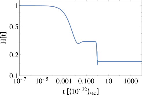
Numerical solutions of the FLRW system (23)-(25) are graphically presented on Fig.3 for the Hubble parameter $H(t)$, and on Fig.4 for the scalar field $u(t)$.

In order to check the viability of our model we will investigate the perturbations of the above FLRW background evolution (23)-(25), in particular focusing on the inflationary observables such as the scalar power spectral index $n_{s}$ and the tensor-to-scalar ratio $r$ (for definitions, see e.g. Ref.[41]). As usual, we introduce the Hubble slow-roll parameters, which in our case using the potential $U_{\rm eff}(u)$ (18) read:

	$\displaystyle\epsilon=\Bigl{(}\frac{U_{\rm eff}^{\prime}(u)}{U_{\rm eff}(u)}\Bigr{)}^{2}=\frac{4\zeta^{2}}{3}\frac{\bigl{(}1/2-\zeta\bigr{)}^{2}}{\bigl{[}\bigl{(}1/2-\zeta\bigr{)}^{2}+\delta/4\bigr{]}^{2}}\;,$		(29)
	$\displaystyle|\eta|=2|\frac{U_{\rm eff}^{\prime\prime}(u)}{U_{\rm eff}(u)}|=\frac{2\zeta}{3}\frac{\bigl{(}1-4\zeta\bigr{)}}{\bigl{[}\bigl{(}1/2-\zeta\bigr{)}^{2}+\delta/4\bigr{]}}\;,$		(30)

where:

$$\zeta\equiv\frac{M_{2}\chi_{2}}{M_{1}}\,e^{-u/\sqrt{3}}\quad,\quad\delta\equiv\frac{8M_{2}\chi_{2}}{M_{1}^{2}}\Lambda_{\rm DE}\;,$$

(31)

with $\Lambda_{\rm DE}$ – the dark energy density (21), and therefore the parameter $\delta$ being very small.

Inflation ends when $\epsilon(u_{f})=1$ for some $u=u_{f}$ whose value (using the short-hand notation $\zeta_{f}\equiv\frac{M_{2}\chi_{2}}{M_{1}}e^{-u_{f}/\sqrt{3}}$) is given by:

$$\zeta_{f}=\frac{1}{2\bigl{(}1+2/\sqrt{3}\bigr{)}}\Bigl{[}1+\frac{1}{\sqrt{3}}-\sqrt{1/3-\bigl{(}1+2/\sqrt{3}\bigr{)}\delta}\Bigr{]}\simeq\frac{1}{2\bigl{(}1+2/\sqrt{3}\bigr{)}}\;.$$

(32)

For the number of $e$-foldings ${\mathcal{N}}=\frac{1}{2}\int_{u_{i}}^{u_{f}}du\;U_{\rm eff}/U_{\rm eff}^{\prime}$ we obtain:

$${\mathcal{N}}=\frac{3}{8}(1+\delta)\Bigl{(}1/\zeta_{i}-1/\zeta_{f}\Bigr{)}-\frac{3}{4}(1-\delta)\log\frac{\zeta_{f}}{\zeta_{i}}+\frac{3}{4}\delta\,\log\Bigl{(}\frac{1-2\zeta_{i}}{1-2\zeta_{f}}\Bigr{)}\;,$$

(33)

where $\zeta_{i}\equiv\frac{M_{2}\chi_{2}}{M_{1}}e^{-u_{i}/\sqrt{3}}$ and $u=u_{i}$ is very large corresponding to the start of the inflation.

Ignoring the very small $\delta$ we have for ${\mathcal{N}}$ approximately:

$${\mathcal{N}}\simeq\frac{3M_{1}}{8M_{2}\chi_{2}}e^{u_{i}/\sqrt{3}}-\frac{\sqrt{3}}{4}u_{i}-\frac{3}{4}\bigl{(}1+2/\sqrt{3}\bigr{)}+\frac{3}{4}\log\Bigl{(}2\bigl{(}1+2/\sqrt{3}\bigr{)}\Bigr{)}\;.$$

(34)

Using the slow-roll parameters (29)-(30), one can calculate the values of the scalar spectral index $n_{s}$ and the tensor-to-scalar ratio $r$, respectively, as functions of the $e$-foldings ${\mathcal{N}}$:

$$r\approx 16\,\epsilon\bigl{(}u_{i}({\mathcal{N}})\bigr{)}\quad,\quad n_{s}\approx 1-6\,\epsilon\bigl{(}u_{i}({\mathcal{N}})\bigr{)}+2\eta\,\bigl{(}u_{i}({\mathcal{N}})\bigr{)}\;,$$

(35)

where $u_{i}({\mathcal{N}})$ is the solution of the transcedental Eq.(34) for $u_{i}$ as a function of ${\mathcal{N}}$. From (35), (34), (29), (30) we find:

	$\displaystyle r\simeq\frac{12}{\Bigl{[}{\mathcal{N}}+\frac{\sqrt{3}}{4}u_{i}({\mathcal{N}})+c_{0}\Bigr{]}^{2}}\;\;\;,\;\;c_{0}\equiv\frac{\sqrt{3}}{2}-\frac{3}{4}\log\Bigl{(}2\bigl{(}1+2/\sqrt{3}\bigr{)}\Bigr{)}\;,$		(36)
	$\displaystyle n_{s}\simeq 1-\frac{r}{4}-\sqrt{\frac{r}{3}}\;\;.\phantom{aaaaaaaaaa}$		(37)

The numerical results for (36)-(37) are depicted on Fig.5.

The different values of the $r$ and $n_{s}$ are compatible with the PLANCK observational data ($0.95<n_{s}<0.97\;,\;r<0.064$) (cf. Ref.[42]).

Indeed, for the viable example of ${\mathcal{N}}=60$ $e$-foldings until the end of inflation we obtain from (34)-(37):

$$n_{s}\approx 0.969\quad,\quad r\approx 0.002\;.$$

(38)

• •

  We proposed a very simple modified gravity model without any initial coupling to matter fields in terms of several alternative non-Riemannian spacetime volume elements within the second order (metric) formalism.

• •

  We show how the non-Riemannian volume elements, when passing to the physical Einstein frame, create a canonical scalar field and produce dynamically a non-trivial inflationary-type potential for the latter possesing a large flat region describing slow-roll inflation and a stable low-lying minimum corresponding to the late universe stage.

• •

  We study the evolution and stability of the cosmological solutions from the point of view of the theory of dynamical systems. Our model predicts scalar spectral index $n_{s}\approx 0.969$ and tensor-to-scalar ratio $r\approx 0.002$ for 60 $e$-folds, which is in accordance with the observational data.

E.N. and S.P. are sincerely grateful to Prof. Branko Dragovich, Prof. Marko Vojinovich and all the organizers of the Tenth Meeting in Modern Mathematical Physics in Belgrade for cordial hospitality. We all gratefully acknowledge support of our collaboration through the academic exchange agreement between the Ben-Gurion University in Beer-Sheva, Israel, and the Bulgarian Academy of Sciences. D.B., E.N. and E.G. have received partial support from European COST actions CA15117, CA16104 and CA18108. E.N. and S.P. are also thankful to Bulgarian National Science Fund for support via research grant DN-18/1.

References

- [1] A. Starobinsky, JETP Lett., 30 (1979) 682 [Pisma Zh. Eksp. Teor. Fiz., 30 (1979) 719].
- [2] A. Starobinsky, Phys. Lett. 91B (1980) 99.
- [3] A. Guth, Phys. Rev. D23 (1981) 347.
- [4] A. Linde, Phys. Lett. 108B (1982) 389.
- [5] A. Albrecht and P Steinhardt, Phys. Rev. Lett. 48 (1982) 1220.
- [6] V. Mukhanov and G. Chibisov, JETP Lett. 33 (1981) 532 [Pisma Zh. Eksp. Teor. Fiz. 33 (1981) 549].
- [7] A. Guth and S. Y. Pi, Phys. Rev. Lett. 49 (1982) 1110.
- [8] S. Weinberg, Cosmology, Oxford Univ. Press, 2008.
- [9] D. Lyth, Cosmology for Physicists, CRC, 2017.
- [10] G. Calcagni, Classical and Quantum Cosmology, Springer, 2017.
- [11] D. Gorbunov and V. Rubakov, Introduction to the Theory of the Early Universe. Hot Big Bang Theory, 2nd Ed., World Scientific, 2018.
- [12] V. Mukhanov and S. Winitzki, Introduction to Quantum Effects in Gravity, Cambridge Univ. Press, 2007.
- [13] S. Perlmutter et al. [Supernova Cosmology Project Collaboration], Astrophys. J. 517 (1999) 565 (astro-ph/9812133).
- [14] E. Copeland, M. Sami and S. Tsujikawa, Int. J. Mod. Phys. D 15 (2006) 1753 (hep-th/0603057).
- [15] S. Weinberg, Ultraviolet divergences in quantum theories of gravitation, in General Relativity. An Einstein Centenary Survey, pp. 790-831, S. Hawking and W. Israel (eds.), Cambridge Univ. Press, 1979.
- [16] M. Green, J. Schwarz and E. Witten, Superstring Theory, vol.1, Cambridge Univ. Press, 1988
- [17] S. Capozziello and V. Faraoni, Beyond Einstein Gravity – A Survey of Gravitational Theories for Cosmology and Astrophysics, Springer, 2011.
- [18] S. Capozziello and M. De Laurentis, Phys. Reports 509, 167 (2011) (arXiv:1108.6266).
- [19] S. Nojiri and S. Odintsov, Phys. Reports 505, 59 (2011).
- [20] E. Berti et.al., Class. Quantum Grav. 32 (2016) 243001 (arXiv:1501.07274).
- [21] S. Nojiri, S. Odintsov and V. Oikonomou, Phys. Reports 692, 1 (2017) (arXiv:1705.11098).
- [22] I.Dimitrijevic, B. Dragovich, Al. Koshelev, Z. Rakic and J. Stankovic, Phys. Lett. 797B (2019) (arXiv:1906.07560).
- [23] N. Bilic, D. Dimitrijevic, G. Djordjevic, M. Miloevic and M. Stojanovci, JCAP 08 (2019) 034 (arXiv:1809.07216).
- [24] E. I. Guendelman and A. Kaganovich, Phys. Rev. D53 (1996) 7020 (arXiv:gr-qc/9605026).
- [25] F.Gronwald, U.Muench, A.Macias, F. Hehl, Phys. Rev. D58 (1998) 084021 (arXiv:gr-qc/9712063).
- [26] E. I. Guendelman, Mod. Phys. Lett. A14 (1999) 1043-1052 (arXiv:gr-qc/9901017).
- [27] E. I. Guendelman and A. Kaganovich, Phys. Rev. D60 (1999) 065004 (arXiv:gr-qc/9905029).
- [28] E.I. Guendelman and A.B. Kaganovich, Ann. Phys. 323 (2008) 866 (arXiv:0704.1998).
- [29] E. I. Guendelman, E. Nissimov and S. Pacheva, Bulg. J. Phys. 41 (2014) 123 (arXiv:1404.4733).
- [30] E. I. Guendelman, E. Nissimov and S. Pacheva, Int. J. Mod. Phys. A30 (2015) 1550133 (arXiv:1504.01031).
- [31] E. I. Guendelman, E. Nissimov and S. Pacheva, Eur. J. Phys. C75, (2015) 472-479 (arXiv:1508.02008).
- [32] E. I. Guendelman, E. Nissimov and S. Pacheva, Eur. J. Phys. C76 (2016) 90 (arXiv:1511.07071).
- [33] E. I. Guendelman, E. Nissimov and S. Pacheva, Int. J. Mod. Phys. D25 (2016) 1644008 (arXiv:1603.06231).
- [34] E. I. Guendelman, E. Nissimov and S. Pacheva, in “Quantum Theory and Symmetries with Lie Theory and Its Applications in Physics”, vol.2 ed. V. Dobrev, Springer Proceedings in Mathematics and Statistics v.225, Springer, 2018 (arXiv:1712.09844).
- [35] E. I. Guendelman, E. Nissimov and S. Pacheva, AIP Conference Proceedings 2075 (2019) 090030 (arXiv:1808.03640).
- [36] M. Spivak, “Calculus On Manifolds – a Modern Approach To Classical Theorems Of Advanced Calculus”, Ch.5, p.126, CRC Press, 2018.
- [37] M. Henneaux and C. Teitelboim, Quantization of Gauge Systems, Princeton Univ. Press, 1991.
- [38] H. Rothe and K. Rothe, Classical and Quantum Dynamics of Constrained Hamiltonian Systems, Ch.3, World Scientific, 2010.
- [39] M. Dabrowski, J. Garecki and D. Blaschke, Ann. Phys. 18 (2009) 13 (arXiv:0806.2683).
- [40] S. Bahamonde, C. G. Boehmer, S. Carloni, E. J. Copeland, W. Fang and N. Tamanini, Phys. Rep. 775-777 (2018) 1 (arXiv:1712.03107).
- [41] S. Nojiri, S. Odintsov and E. Saridakis, Phys. Lett. 797B (2019) 134829 (arXiv:1904.01345).
- [42] Y. Akrami et al. [Planck Collaboration], arXiv:1807.06211 .