Non-perturbative analytical diagonalization of Hamiltonians with application to coupling suppression and enhancement in cQED
Abstract
Deriving effective Hamiltonian models plays an essential role in quantum theory, with particular emphasis in recent years on control and engineering problems. In this work, we present two symbolic methods for computing effective Hamiltonian models: the Non-perturbative Analytical Diagonalization (NPAD) and the Recursive Schrieffer-Wolff Transformation (RSWT). NPAD makes use of the Jacobi iteration and works without the assumptions of perturbation theory while retaining convergence, allowing to treat a very wide range of models. In the perturbation regime, it reduces to RSWT, which takes advantage of an in-built recursive structure where remarkably the number of terms increases only linearly with perturbation order, exponentially decreasing the number of terms compared to the ubiquitous Schrieffer-Wolff method. In this regime, NPAD further gives an exponential reduction in terms, i.e. superexponential compared to Schrieffer-Wolff, relevant to high precision expansions. Both methods consist of algebraic expressions and can be easily automated for symbolic computation. To demonstrate the application of the methods, we study the ZZ and cross-resonance interactions of superconducting qubits systems. We investigate both suppressing and engineering the coupling in near-resonant and quasi-dispersive regimes. With the proposed methods, the coupling strength in the effective Hamiltonians can be estimated with high precision comparable to numerical results.
I Introduction

Deriving effective models is of fundamental importance in the study of complex quantum systems. Often, in an effective model, one decouples the system of interest from the ancillary space, as shown in Figure 1. The dynamics are then studied within the effective subspace, which is usually much easier than in the original Hilbert space, and provides fundamental information such as conserved symmetries, entanglement formation, orbital hybridization, computational eigenstates, spectroscopic transitions, effective lattice models, etc. In terms of the Hamiltonian operator, an effective compression of the Hilbert space can be achieved by diagonalization or block diagonalization.
When the coupling between the system and ancillary space is small compared to the dynamics within the subspace, the effective model is often derived by a perturbative expansion. In the field of quantum mechanics, a ubiquitous expansion method that enables reduced state space dimension is the Schrieffer-Wolff Transformation (SWT) [1, 2], also known in various sub-fields as adiabatic elimination [3], Thomas-Fermi or Born-Oppenheimer approximation [4, 5], and quasi-degenerate perturbation theory [6]. Finding uses throughout quantum physics, SWT can be found in atomic physics [3], superconducting qubits [7, 8], condensed matter [2], semiconductor physics [9], to name a few.
The SWT method is however limited to regimes where a clear energy hierarchy can be found and therefore fails to converge for a wide variety of physical examples. In particular, for infinite-dimensional systems such as coupled harmonic and anharmonic systems (e.g., in superconducting quantum processors), the abundance of both engineered and spurious resonances motivates the use of other techniques. Moreover, even when perturbation theory is applicable, the number of terms in the expansions grows exponentially as the perturbation level and therefore are not practically usable in many instances.
In this article, we introduce a new symbolic algorithm, Non-Perturbative Analytical Diagonalization (NPAD), that allows the computation of closed-from, parametric effective Hamiltonians in a finite-dimensional Hilbert space with a guarantee for convergence. The method makes use of the Jacobi iteration and recursively applies Givens rotations to remove all unwanted couplings. In the perturbative limit, it reduces via BCH expansion to a variant of SWT, which we refer to as the Recursive Schrieffer-Wolff Transformation (RSWT). For this method, the number of commutators grows only linearly with respect to the perturbation order, in contrast to the exponential growth in the traditional approach. Both methods can be used in low-order expansions to provide compact analytical expressions of effective Hamiltonians; or, alternatively, higher-order expansions that allow for fast parametric design [10] and tuning [11] of effective Hamiltonian models (and, e.g., subsequent automatic differentiation). As illustrated in Figure 1, with the two methods, one can tune the system for engineered decoupling or enhanced controlled coupling.
The key insight of our work is that the iteration step in forming the effective model can be applied recursively, i.e. after each step the transformed Hamiltonian is viewed as a new starting point and determines the next step. Moreover, each step can act on a chosen single state-to-state coupling at a time, thereby providing an exact elimination of the term. In this regard, this can be understood as a generalization of the well-known numerical Jacobi iteration used for diagonalization of real symmetric matrices [12], which has also found use for Hermitian operators [13, 14]. Similar ideas have also been widely used in the orbital localization problem [15].
As demonstrations of the practical utility of the methods, we study superconducting qubits, which are especially relevant for robust parametric design methods, not only because they are prone to spurious resonances [16, 17, 18], but because they can be readily fabricated across a very wide range of energy scales [19, 20].
We investigate both the near-resonant regime and in the quasi-dispersive regime, focusing on the ZZ and cross-resonance interaction. In the near-resonant regime, we consider the two-excitation manifold and compute accurate approximations of the ZZ interaction strength applicable to the full parameter regime for gate implementation [21, 22, 23, 24]. In the second scenario, we study the suppression of ZZ interactions [10, 25, 26, 27, 28, 29, 30, 31, 32, 33, 34, 35, 36, 37, 38, 39, 40, 41] in the traditional setup of resonator mediated coupling without direct qubit-qubit interaction. The result shows that the ZZ interaction can be suppressed without resorting to additional coupling in a regime where the qubit-resonator detuning is comparable to the qubit anharmonicity, described by an equation of a circle. Extending the applications to block diagonalization, we then compute the coupling strength of a microwave-activated cross-resonant interaction. We show that, with only 4 Givens rotations, we can diagonalize the drive and achieve accurate estimation in the regime where the perturbation method fails.
This paper is organized as follows: In Section II, we present the mathematical methods, NPAD and RSWT, for diagonalization and obtaining effective Hamiltonian models. We also briefly discuss generalizing the two methods to block diagonalization in Section II.3. Next, in Section III, we demonstrate the applications to superconducting systems. We study the ZZ interaction for generating entanglement in the near-resonant regime (Section III.1), and in the (quasi-) dispersive regime for suppressing cross-talk noise (Section III.2). The computation of the cross-resonance coupling strength is presented in Section III.3. We conclude and give an outlook of other possible applications in Section IV.
II Mathematical methods
II.1 Non-perturbative Analytical Diagonalization
In this subsection, we introduce the NPAD for symbolic diagonalization of Hermitian matrices and discuss how it can be applied to obtain effective models.
In this algorithm, a Givens rotation is defined in each iteration to remove one specifically targeted off-diagonal term. By iteratively applying the rotations, the transformed matrix converges to the diagonal form. The rotation keeps the energy structure when the off-diagonal coupling is small while always exactly removing the coupling even when it is comparable to or larger than the energy gap. Compared to the Jacobi method used in numerical diagonalization [12, 14, 13], we truncate the iteration at a much earlier stage. As each iteration consists only of a few algebraic expressions, the algorithm produces a closed-form, parametric expression of the transformed matrix.
We start from a two-by-two Hermitian matrix and define a complex Givens rotation that diagonalizes it. Then, we generalize the rotation to higher-dimensional matrices, discuss the convergence of the iteration, and how to use it as a symbolic algorithm. In Section III.1, we show a concrete application where we apply NPAD with only two rotations to approximate the energy spectrum of a near-resonant quantum system which can not be studied perturbatively.
II.1.1 Givens rotations


We consider a two-by-two Hermitian matrix
| (1) |
where , , and are real numbers. The matrix can be decomposed in the Pauli basis as
| (2) |
which can be illustrated in a Bloch sphere with the radius (omitting the identity) as shown in Figure 2a. Without loss of generality, we assume that and absorb the sign into the complex phase.
The diagonalization can be understood as a rotation on the Bloch sphere to the North or South pole. In particular, if , it is rotated to the North pole, and otherwise to the South pole, avoiding unnecessarily flipping the energy level during the diagonalization. This rotation is performed around the axis with the angle . As an illustration, for , the rotation is denoted by a blue arrow in Figure 2a.
The unitary transformation that diagonalizes the matrix is given by
| (3) |
where is referred to as the generator of the rotation. The transformation satisfies with the diagonalized matrix. We refer to as a Givens rotation [42]. Notice that in most literature, the Givens rotation is defined with . Here we use this more general (Hermitian) definition as it shares many common properties.
The computation of the unitary consists only of elementary mathematical functions, as illustrated in Figure 2b. This is critical for it to be used as a building block for a symbolic algorithm. As we will see later, by concatenating this building block, a parameterized expression can be generated for an arbitrary Hermitian matrix.
II.1.2 Simplified formulation
In practice, the inverse trigonometric function in the expression of is often avoided by using the trigonometric identities
| (4) |
with . We then rewrite Eq. 4 as
| (5) |
with . We choose the root with smaller norm for the convenience that the rotation will not flip the two energy levels 111In numerical implementation, it is often written as for numerical stability when .:
| (6) |
In this way, the parameters and in the Givens rotation can be calculated directly from and using algebraic expressions. It is also evident in Eq. 6 that the rotation angle is bounded by .
II.1.3 The iterative method
We now apply the Givens rotation to remove the ()-th entry of a general Hermitian matrix . The parameters are chosen to be consistent with Eq. 1, i.e., and . For simplicity, we use the notation , , and . We write the Givens rotation as
| (7) |
where the diagonal elements are all 1 except for two entries and . All other entries not explicitly defined are 0.
Applying this unitary transformation with eliminates the off-diagonal entry , i.e., . It renormalizes the energies such that
| (8) |
However, this will also mix other entries on the -th rows and columns, given by
| (9) | ||||||
| (10) |
with .
One can diagonalize the matrix by applying the rotation with the corresponding parameters iteratively on the largest remaining non-zero off-diagonal entry, which is referred to as the Jacobi iteration [12]. That is, we can iteratively solve for the eigenenergies by picking the next largest off-diagonal element, e.g., , and applying another Givens rotation, as summarized in algorithm 1.
-
1.
find the target coupling ;
-
2.
define , and such that
; 4. , ; 5. define according to Eq. 7; 6. ;
In practice, the above definition of the Jacobi iteration can be relaxed. For instance, the next target does not always have to be the largest element. In fact, the order of the rotations does not affect the convergence, as long as all terms are covered in the iteration rules (e.g., cyclic iterations on all off-diagonal entries) [13]. However, performing the rotation first on large elements usually increases the convergence rate. This can be seen by studying the norm of all off-diagonal terms . Since we have for and , each Givens rotation reduces the norm of all off-diagonal terms:
| (11) |
If () is chosen so that is larger than the average norm among the off-diagonal terms, one obtains [13]
| (12) |
where is the total number of off-diagonal terms. Therefore, the algorithm converges exponentially. Moreover, if the off-diagonal terms are much smaller than the energy gap, the convergence becomes even faster, i.e., exponentially fast with a quadratic convergence rate [14]. This leads to an efficient variant of the Schrieffer-Wolff-like methods, as described in Section II.2.
From the above analysis, we also see that the Givens rotation does not have to exactly zero the target coupling. Instead, it only needs to reduce the total norm. Therefore, if the structure of the Hamiltonian is known, rotations can be grouped such that all rotations within one group are constructed from the same Hamiltonian and then applied recursively. We will also explore this possibility in concrete examples later in the article.
As a machine-precision, numerical diagonalization algorithm, the Jacobi iteration is slower than the QR method for dense matrices. However, in many problems in quantum engineering, the Hamiltonian is often sparse and it is known in advance which interaction needs to be removed. It is not always necessary to compute the fully diagonalized matrix but only to transform it into a frame where the target subspace is sufficiently decoupled from the leakage levels. Therefore, an iterative method where each step is targeted at one off-diagonal entry is of particular interest.
As a symbolic method, we can truncate the Jacobi iteration at a very early stage to obtain closed-formed parametric expressions. It will also correctly calculate the renormalized energy and other couplings while keeping the energy structure in the perturbative limit, as will be discussed in Section II.2.
II.2 Recursive Schrieffer-Wolff perturbation method
In the previous subsection, we introduced NPAD that produces a closed-form, parametric expression of an approximately diagonalized matrix. Here, we show that in the perturbative limit, where the coupling is much smaller than the bare energy difference, the Jacobi iteration reduces to a Schrieffer-Wolff-like transformation. Interestingly, the recursive nature of the Jacobi iteration is preserved in this limit. Instead of looking for one generator that diagonalizes the full matrix as in the traditional Schrieffer-Wolff transformation (SWT), an iteration is constructed such that every time only the leading-order coupling is removed. We refer to it as recursive Schrieffer-Wolff transformation (RSWT) because of the recursive expression it produces. We also show that RSWT demonstrates an exponential improvement in complexity compared to SWT for perturbation beyond the leading order. In Section III.2, we demonstrate an application of RSWT in estimating the ZZ interaction between two Transmon qubits in a dispersive regime.
II.2.1 Givens rotation in the perturbative limit
In the perturbative limit, compared to in Eq. 7, it is more convenient to specify the generator defined in Eq. 3. For the Givens rotation the corresponding generator has two non-zero entries
| (13) |
all other entries being 0. In addition, assuming that we only aim at removing the leading-order off-diagonal terms, we define a generator
| (14) |
where the sum over denotes all pairs of non-zero off-diagonal entries in . The assumption of perturbation indicates that . In this case, the unitary generated by still eliminates all the leading-order coupling because
| (15) |
This generator is identical to the generator of the leading-order SWT. One can verify that where and are the diagonal and off-diagonal parts of . By expanding the transformation using the BCH formula
| (16) |
and truncating the series at , one obtains the leading-order SWT.
The difference between RSWT and SWT appears when one considers higher-order perturbation. In SWT, one expands the transformed Hamiltonian and the generator perturbatively as a function of a small parameter and collects terms of the same order on both sides of Eq. 16. However, here, the generator is predefined and it only eliminates the leading-order coupling. Similar to the Jacobi iteration, we treat the transformed Hamiltonian as a new Hermitian matrix and perform another round of leading-order transformation as the next iteration. This results in a recursive expression for , which is still a closed-form expression. The remaining off-diagonal terms can always be removed by the next iteration if the truncation level of BCH formula is high enough to guarantee sufficient accuracy. We present the iteration of RSWT in detail in the next subsection and show that it simplifies the calculation for perturbation beyond the leading order.
II.2.2 The RSWT iterations
In the following, we outline the iterative procedure of the RSWT. We denote the initial matrix as step zero, with the notation , and . The parameter is the dimensionless small parameter used to track the perturbation order. Assume that we want to compute the perturbation to the eigenenergy up to the order . We refer to this as the -perturbation. Given the Hamiltonian of iteration , , we can compute the next iteration as follows.
We first define a generator according to Eq. 14 such that , where and are the diagonal and the off-diagonal part of . As the energy gap always stays at under the assumption of small perturbation, is of the same order as . Notice that is generated from the perturbed matrix in the previous iteration, , in contrast to the unperturbed matrix as in SWT.
Then, the next level of perturbation is computed with
| (17) |
where is the nested commutator defined by
| (18) |
and . The truncation level of the BCH expansion will be defined explicitly later. Because by construction, we have for all and
| (19) |
Therefore, plugging in Eq. 19 into Eq. 17 simplifies it to
| (20) |
Notice that starts from 1 in the sum, which means that all coupling terms at the same order of are removed and the order of the remaining coupling, , is squared. This iteration is applied until the desired order is reached, as summarized in algorithm 2.
-
1.
; ;
-
2.
initialize a zero matrix ;
;
To ensure that the truncation of the BCH is accurate up to the order , for the th iteration, we need to choose the truncation , which ensures that . This maximal level is halved every time the iteration step increases because the remaining coupling is quadratically smaller. This means that, in contrast to SWT, the first iteration has the largest number of terms in RSWT. In appendix A, we show that, if , the error of the truncation in Eq. 20 is bounded by
| (21) |
where the is Eq. 20 in the limit .
II.3 Block diagonalization
Both the NPAD and the RSWT methods introduced in the previous sections can be designed to only target a selected set of off-diagonal terms and, hence, used for block-diagonalization. This is especially useful to engineer transversal coupling in a subsystem and leave the remaining levels as intact as possible. Here, we briefly discuss these generalizations. Notice that it is always possible to first diagonalize the matrix and then reconstruct the block diagonalized form that satisfies certain conditions, for instance as in Ref. [44]. In the following, we discuss only methods that do not diagonalize the matrix first.
In NPAD, by construction, each rotation removes one off-diagonal element. With Givens rotations only applied to the inter-block elements, an iteration for block diagonalization can be defined. The norm of all off-diagonal entries, , is still monotonously decreasing according to Eq. 11. Hence, a limit exists and its convergence is also the convergence of the block diagonalization. However, the convergence is not always monotonous with respect to the norm of all inter-block terms. This is because a Givens rotation may rotate a large intra-block term into an inter-block entry. Therefore, the algorithm may not always converge faster than the full diagonalization would. Nevertheless, if the dominant coupling terms in the Hamiltonian are known, the Jacobi iteration can be designed to target at those to realize an efficient block-diagonalization. In Section III.3, we show an example of this in computing the cross-resonance coupling strength through NPAD.
For perturbation, RSWT can be applied as a block diagonalization method under the constraint that both the inter-block and the intra-block coupling are much smaller than the inter-block energy gap. This can be achieved by slightly modifying the RSWT iterations: We first separate the diagonal, the intra-block and the inter-block terms: . Next, in algorithm 2 we only define for those non-zero entries in , i.e. the couplings we wish to remove. And in the last step we replace Eq. 20 with
| (22) |
In this definition, the leading inter block coupling is of the order . As we do not remove the intra-block coupling, we still get . Therefore, the remaining coupling is , i.e. the perturbation order is increased by one, instead of being squared as in the case of full diagonalization. Therefore, the exponential reduction of the number of commutators does not always apply in the case of block diagonalization. However, notice that the small parameter here is defined as the (largest) ratio between the inter-block couplings and gaps, which is usually much smaller than those within the block. Hence, if carefully designed, the convergence can still surpass the full diagonalization in the first few perturbative orders.
II.4 Comparison between different methods
To help understand the proposed methods, we here discuss the difference between them and the traditional methods. We first compare RSWT with traditional SWT and then NPAD with the perturbation methods.
For RSWT, with the same target accuracy, e.g., , it should provide the same expression as from SWT, up to the error . However, compared to the SWT, RSWT requires a much smaller number of iterations and commutators. To reach , SWT needs iterations, while RSWT only needs because of the quadratic convergence rate. More importantly, the total number of commutators grows only linearly for RSWT, compared to the exponentially fast growth for SWT [7].
Intuitively, this is because RSWT uses the recursive structure and avoids unnecessary expansions of the intermediate results. Mathematically, this can be seen from the following two aspects: First, in RSWT, each iteration improves the perturbation level from to , instead of . Hence, the number of iterations increases only logarithmically with respect to the perturbation order, as seen in the definition of in algorithm 2. This is because we always treat the transformed matrix as a new one and remove the leading-order coupling. It is consistent with the quadratic convergence rate of the Jacobi iteration with small off-diagonal terms. Second, in RSWT, the generator is only used at the current iteration. Hence, there are no mixed terms such as , in contrast to SWT.
The total number of commutators required to reach level is shown in Table 1, where we have taken into consideration that if is known, computing only requires one additional commutator. The detailed calculation is presented in appendix B.
The NPAD method, on the other hand, uses non-linear rotations to replace the linear perturbative expansion. More concretely, in the Jacobi iteration, by targeting only one coupling in each recursive iteration, the unitary transformation can be analytically expressed as a Givens rotation, thus avoiding the BCH expansion in Eq. 16. Therefore, it efficiently and accurately captures the non-perturbative interactions in the system.
To compare it with the perturbation methods, we estimate the number of operations required for NPAD in the perturbative regime. Assume we construct the Jacobi iteration from the coupling terms used in generating an in RSWT. Applying those unitaries is, to the leading order, the same as applying one RSWT iteration. A single Givens rotation on a Hamiltonian takes operations, where is the matrix size. Thus, the cost for computing the effective Hamiltonian after rotations is the same as computing one commutator , up to a constant factor. Because the Givens rotation avoids the BCH expansion, there is no nested commutators and the total number operations is with the number of iterations in algorithm 2. Hence the number of terms scales logarithmically with respect to instead of linearly as for RSWT, i.e., a super-exponential reduction compared to SWT (Table 1). However, the non-linear expressions provided by NPAD are usually harder to simplify and evaluate by hand compared to the rational expressions obtained from perturbation.
From the above discussion, one can see that it is also straightforward to combine NPAD with perturbation. Instead of fully diagonalizing the matrix, the Jacobi iteration can be designed to remove only the dominant couplings and combined with perturbation methods to obtain simplified analytical expressions. In fact, this is often used implicitly in the analysis when, e.g., a strongly coupled two-level system is perturbatively interacting with another quantum system. The Jacobi iteration suggests that this can be generalized systematically to more complicated scenarios.
| 2 | 3 | 4 | 5 | 6 | 7 | 8 | |
|---|---|---|---|---|---|---|---|
| SWT | 1 | 4 | 11 | 26 | 57 | 120 | 247 |
| RSWT | 1 | 2 | 4 | 5 | 7 | 8 | 11 |
| NPAD | 1 | 1 | 2 | 2 | 2 | 2 | 3 |
III Physical applications
In this section, we use the methods introduced in Section II to study the ZZ interaction in two different parameter regimes. In a two-qubit system, the ZZ interaction strength is defined by
| (23) |
where denotes the eigenenergy of the two-qubit states . The Hamiltonian interaction term is written as , acting on the two qubits. Typically, in superconducting systems, it arises from the interaction of the state with the non-computational state in the physical qubits, and can both be used as a resource for entangling gates [21, 22, 23, 24] or viewed as cross-talk noise that needs to be suppressed [25, 26, 27, 28, 29, 30, 31, 32, 33, 34, 35, 36, 37, 38, 39, 40, 41].
III.1 Effective ZZ entanglement from multi-level non-dispersive interactions
In this first application, we apply the NPAD method described in Section II.1 to study a model consisting of two directly coupled qubits in the near-resonant regime, where the ZZ interaction can be used to construct a control-Z (CZ) gate (see Figure 1 block B) [21, 22, 23, 24]. We show that, with two rotations, NPAD provides an improvement on the estimation of the interaction strength for at least one order of magnitude, compared to approximating the system as only a single avoided crossing between the strongly interacting levels, as is standard in the literature. In addition, if one of the non-computational bases is comparably further detuned than the other, the correction takes the form of a Kerr nonlinearity, with a renormalized coupling strength accounting for the near-resonant dynamics.
We consider the Hamiltonian of two superconducting qubits that are directly coupled under the rotating-wave [45, 46] and Duffing [47] approximations:
| (24) |
where , , are the annihilation operator, the qubit bare frequency and the anharmonicity, respectively. The parameter denotes the coupling strength. In this Hamiltonian, the sum of the eigenenergies is always a constant because of the symmetry. Hence, the ZZ interaction comes solely from the interaction between the state and the non-computational basis and . If the frequency is tuned so that the state is close to one of the non-computational states, the coupling will shift the eigenenergy, leading to a large ZZ interaction (Figure 3a).
For simplicity, we consider the Hilbert subspace consisting of , , and write the following Hamiltonian
| (25) |
The parameters in the diagonal elements are given by and . To keep the result general, we use two different coupling strengths and , although according to Eq. 24 they both equal . Without loss of generality, we assume the state is comparably further detuned from the other two, i.e. . If in contrast is further detuned, one can exchange the and in the matrix and redefine and accordingly. Notice that this Hamiltonian is different from a system [3], where coupling exists only between far detuned levels.
To implement the CZ gate, one tunes the qubit frequency so that the states and are swept from a far-detuned to a near-resonant regime. Hence, the perturbative expansion diverges and cannot be used. A naive approach is to neglect the far-detuned state and approximate the interaction as a single avoided crossing. In this case, is approximated by
| (26) |
However, the interaction results in an error that, in the experimentally studied parameter regimes, can be as large as 10%, as shown in Figure 3b.
In the following, we show that with only two Givens rotations, one can obtain an analytical approximation, with the error reduced by one order of magnitude. The correction can be understood as a Kerr non-linearity with a renormalized coupling strength.
To get an accurate estimation of the ZZ interaction , we need to calculate the eigenenergy of by eliminating its coupling with the other two states. Therefore, we will make two rotations sequentially on the entry and , given by
| (27) |
where and are Givens rotations (Eq. 3) constructed for eliminating the entries and . Because the matrix is real symmetric, the phase in Eq. 3 is 0.
The first transformed Hamiltonian, , takes the form
| (28) |
where is the eigenenergy for diagonalizing the two-level system of and , consistent with Eq. 26. The notations used is the same as in Section II.1.3. In this frame, the coupling between and is reduced to , where is given by the non-linear expression
| (29) |
This non-linearity is crucial for the accurate estimation of the eigenenergy.
The second rotation further removes this renormalized coupling , giving
| (30) |
Including the new correction, , the eigenenergy of state reads
| (31) |
In Figure 3b, we plot the error of the estimated interaction strength using typical parameters of superconducting hardware, compared to the numerical diagonalization . An improvement of at least one order of magnitude is observed compared to traditional methods.
Following the assumptions that , Eq. 31 simplifies to
| (32) |
We see that the correction takes the form of a Kerr non-linearity [48], but with a renormalized coupling strength . This non-linear factor accounts for the dynamics between and in the near-resonant regime. The same effect can be observed in higher levels where similar three-level subspaces exist. This approximation is plotted as a dashed curve in Figure 3b.
The error of this estimation comes both from the expansion of the square root in Eq. 31 as well as from the remaining coupling in . The former can be approximated by the next order expansion
| (33) |
For the latter, we consider the remaining coupling in between and , which reads . In the limit , we have , indicating that this coupling is much smaller than the energy difference. Hence, further correction can be estimated by
| (34) |
The contribution of the other remaining coupling between and is much smaller due to the large energy gap. Since is one order smaller than the , will be the dominant error. We plot the region below this error in Figure 3b as a shaded background.
For the more general cases without assuming , it is hard to provide an error estimation due to the non-linearity. However, the result in Figure 3b indicates that Eq. 31 still shows a good performance in other parameter regimes commonly used in superconducting hardware, with an error smaller than 3%. We also observe that an improvement for another order of magnitude can be achieved by introducing a third rotation again on the entry .


III.2 ZZ coupling suppression in the quasi-dispersive regime
In this second example, we use the two methods to investigate the suppression of ZZ cross-talk with the qubit-resonator-qubit setup in the dispersive cQED regime, which corresponds to Figure 1 block A. We demonstrate that in the traditional setup without direct inter-qubit coupling, the ZZ interaction defined in Eq. 23 can still be zeroed in a quasi-dispersive regime by engineering the two parameters of qubit-resonator detuning. The zero points are described by an equation of a circle in the -perturbation. To accurately capture the interaction strength in the quasi-dispersive regime, we also compute with RSWT the -perturbation and show that the NPAD method with only 8 Givens rotations provides an expression with similar accuracy.
We consider a Hamiltonian of two superconducting qubits connected by a resonator:
| (35) | ||||
Due to the finite detuning between the resonator and the qubits, a static ZZ interaction exists even if there is no additional control operation on the system. In order to implement high-quality quantum operations, this interaction needs to be sufficiently suppressed.
Several approaches have been developed to suppress the ZZ interaction. One way is to add a direct capacitive coupling channel in parallel with the resonator [34, 27, 33, 32, 30, 36, 49, 28, 31, 35, 29]. By engineering the parameters, the two interaction channels cancel each other. The interaction can either be turned on through a tunable coupler or through the cross resonant control scheme. The second approach is to choose a hybrid qubit system with opposite anharmonicity, which allows parameter engineering to suppress the ZZ interaction. One implementation is using a transmon and a capacitively shunt flux qubit (CSFQ) [25, 26]. Other methods include using additional off-resonant drive [39, 40, 41] and different types of qubits have also been proposed [38].
Most of the above works are based on the strong dispersive regime, where the resonator is only weakly coupled with the qubits. In this regime, the ZZ interaction strength is only determined by the effective interaction with the two non-computational qubit state, and [7]
| (36) |
where is the qubit-resonator frequency detuning, the anharmonicity and the effective coupling strength between the physical qubit state and . They are obtained by performing a leading order SWT and effectively decouple the resonator from the two qubits. In this regime, it is impossible to achieve zero ZZ interaction unless the two anharmonicity adopt different signs.


However, Eq. 36 is only valid when ignoring the higher level of the resonator. If we reduce the qubit detuning so that it becomes comparable with the anharmonicity , the second excited state of the resonator comes into the picture and can be used to suppress the ZZ interaction, also known as the quasidisq regime [10, 37]. We identify this regime as the quasi-dispersive regime because is manufactured larger than , e.g. in superconducting qubits with weak anharmonicity such as Transmons, though we show the same analysis can also hold for stronger anharmonicities. As a result, the calculation of cannot be treated by only the leading-order SWT. In particular, we will see that, in the straddling regime, where , the interaction with the second excited resonator state leads to a -perturbative correction that can be used to suppress the ZZ interaction.
In the following, we first use the -perturbation to qualitatively understand the energy landscape and then investigate the higher-order corrections. For the -perturbation, using RWST, we only need 2 iterations and evaluate 4 commutators instead of 3 iterations and 11 commutators, as for traditional perturbation (Table 1).
In fact, the traditional approach that first approximates the system as an effective qubit-qubit direct interaction and then applies another perturbation to obtain the ZZ strength is also a two-step recursion [7]. However, for simplicity, it neglects the resonator states in the second perturbation. As detailed in appendix C, adding the resonator states, we obtain a better estimation for the quasi-dispersive regime. The result is consistent with the diagrammatic techniques used in [50, 25].
To illustrate the energy landscape, we write the interaction strength as
| (37) |
with . The first two terms coincide with Eq. 36 in the strong dispersive regime, up to .
Assuming and set in Eq. 37, we obtain an equation of a circle that describes the location of the zero points
| (38) |
where and . In this -perturbation, the zero-points depend only on the anharmonicity but not on the coupling strength . Equation 38 indicates that the ZZ interaction can be suppressed by varying the sum and difference of the two qubit-resonator detunings, as illustrated in Figure 4a. Because the perturbative approximation is only valid away from the resonant lines, the useful part of the parameter regime is the half-circle with , in particular, the region marked by the grey box in Figure 4a.
[figure]style=plain,subcapbesideposition=top
[ ]

\sidesubfloat[ ]

In addition, we also studied different contributions to the ZZ interaction. In Figure 5, we plot the strong dispersive approximation, the -perturbation as well as the contribution of second excited qubit and resonator state to (see appendix C for analytical expressions). One observes from the plot that, in the quasi dispersive regime, the increasing virtual interaction with the second excited resonator state acts against the interaction with the second excited qubit states. Notice that all contributions to are virtual interactions of the second excited state, i.e., , as illustrated in Figure 5.
Although the -perturbation gives insight into the different contributions to the energy shift, perturbation beyond the order also has a non-negligible contribution in the quasi-dispersive regime. Since RSWT requires considerably fewer commutators, we are able to compute the -perturbation, with only two iterations and 7 commutators (see Table 1). The -perturbation captures the location of the minimum more accurately, but still shows a false minimum close to the resonant regime, as shown in Figure 4b.
Apart from perturbation, we also apply NPAD to compute the interaction strength. We first define 4 Givens rotations with respect to the direct qubit-resonator coupling terms from the original Hamiltonian. The rotations are then applied sequentially to obtain the first effective Hamiltonian. Next, we apply another 4 rotations targeted at the two-photon couplings, such as the effective qubit-qubit coupling. The indices of those 8 rotations are listed in the first two columns of Table 2. These two steps are equivalent to the two iterations in RSWT. However, the recursive Givens rotations replace the BCH expansion, resulting in a much simpler calculation. Illustrated in Figure 4b, the approximation with those 8 rotations is as good as the -perturbation, but without the false minimum. Both capture the zero points very well compared to the numerical diagonalization, where the 4 lowest levels are included for each qubit and the resonator.
With those calculations, we can then investigate the effect of the high order corrections. We find that, for instance, shifts the zero point to the regime of smaller frequency detuning, corresponding to shrinking the half-circle in the numerical calculation in Figure 4a. In addition, for stronger coupling strength, the dip becomes narrower, which indicates a trade-off between the interaction strength and feasibility of qubit fabrication [51]. A detailed description of the effect of higher-order perturbation in the quasi-dispersive regime is presented in appendix D.
Overall, our investigation reveals different contributions to the ZZ interaction and provides tools to study the energy landscape in this quasi-dispersive regime. Because of the comparably smaller detuning, operations on this regime provide stronger interactions for entangling gates, and hence may achieve a better quantum speed limit for universal gate sets, i.e. without sacrificing local gates [10].
| static | |
|---|---|
| Step 1 | Step2 |
| 010-100 | 011-200 |
| 001-100 | 001-010 |
| 011-101 | 011-002 |
| 011-110 | 011-020 |
| driving |
|---|
| 00-10 |
| 01-11 |
| 10-20 |
| 11-21 |
III.3 The cross-resonance coupling strength
Following the previous examples, we here study superconducting qubits under an external cross-resonance drive. The cross-resonance interaction is activated by driving the control qubit with the frequency of the target qubit, which has been studied intensively and demonstrated in various experiments [52, 53, 54, 55, 56, 33]. In the two-qubit subspace, the dominant Hamiltonian term is written as a Pauli matrix , which generates a CNOT gate up to single-qubit corrections. Therefore, ideally, only the population of the target qubit will change after the gate operation. The effective model is usually derived by block diagonalizing the non-qubit leakage levels as well as the population flip of the control qubit [7, 8, 57]. The coupling strength is then characterized by the coefficient of the Hamiltonian term.
The analytical block diagonalization of the Hamiltonian is only possible when neglecting all the non-qubit levels. Hence, perturbative expansion is often used, where the small parameter is defined as , i.e., the ratio between the drive amplitude and the qubit-qubit detuning. However, to achieve fast gates, the qubit-qubit detuning is often designed to be small, ranging from 50 MHz to 200 MHz. Therefore, the perturbative diagonalization only works well for a weak drive.
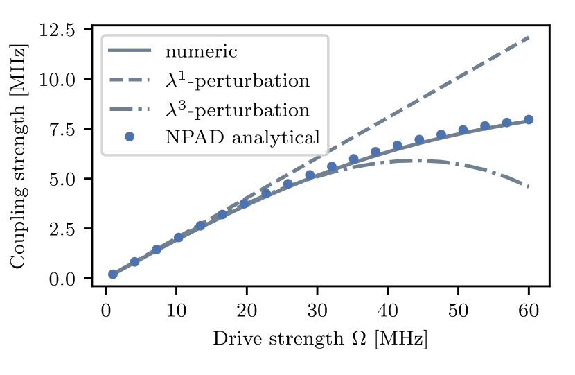
In the rest of this subsection, we show that with only 4 two-by-two Givens rotations on the single-photon couplings, we can block-diagonalize the drive term and obtain an estimation of the coupling strength as good as the numerical result and far above the perturbative regime.
We start from the static Hamiltonian in Eq. 24 and define a driving Hamiltonian in the rotating frame
| (39) |
The full Hamiltonian is then written as where with the driving frequency [7]. To compute the interaction strength, both the qubit-qubit effective interaction and the drive on the control qubit need to be diagonalized. In particular, the second one can be as large as the energy gap and dominant in the unwanted couplings [57]. For simplicity, we assume is small and diagonalize it with a leading-order perturbation, discarding all terms smaller than . In this frame, one obtains a interaction that increases linearly with the drive strength [7]. This is equivalent to moving to the eigenbases of the idling qubits and allows us to focus on applying NPAD to the drive . The same method used in Section III.2 can be applied here to improve this approximation.
Targeting the dominant drive terms listed in the right column of Table 2, we construct 4 Givens rotations. The rotations are constructed with respect to the same Hamiltonians and then applied iteratively as separate unitaries. The obtained interaction strength reads
| (40) | ||||
with , and . The rotation angles are defined by the drive strength and .
This analytical coupling strength is plotted in Figure 6, compared with the perturbative expansions in Ref. [7] and numerical block-diagonalization. The result matches well with the numerical calculation, even when the ratio is approaching one. On the contrary, the perturbative expansion shows a large deviation as the driving power increases. The numerical block-diagonalization is implemented using the least action method [44, 7, 29]. To our surprise, although no least action condition is imposed on the Jacobi iteration, the method automatically follows this track and avoids unnecessary rotations. This suggests that the Jacobi iteration chooses an efficient path of block-diagonalization.
Notice that in the above example, no rotations are performed for levels beyond the second excited state because they are not directly coupled to the qubit subspace. In other parameter regimes, more couplings terms may become significant and need to be added to the diagonalization. For instance, the two-photon interaction between and of the control qubit will be dominant in the regime where [8]. The fact that high precision can be achieved with only rotations on the single-photon couplings in this example also indicates that the dominant error of perturbation lies in the BCH expansion used in diagonalizing the strong single-photon couplings, rather than in higher levels or high-order interactions.
IV Conclusion and outlook
We introduced the symbolic algorithm NPAD, based on the Jacobi iteration, for computing closed-form, parametric expressions of effective Hamiltonians. The method applies rotation unitaries iteratively on to a Hamiltonian, with each rotation recursively defined upon the previous result and removing a chosen coupling between two states. Compared to perturbation, it uses two-by-two rotations to avoid the exponentially increasing commutators in the BCH expansion. In the perturbative limit, the method reduces to a modified form of the Schrieffer-Wolff transformation, RSWT, that inherits the recursive structure of the Jacobi iteration. The recursive structure avoids unnecessary expansion and results in an exponential reduction in the number of commutators compared to the traditional perturbative expansion. The two methods can also be combined as a hybrid method, where NPAD is used to remove strong couplings while RSWT is applied afterwards to effectively eliminate the remaining weak coupling.
Applying these methods to superconducting qubit systems, we showed that high precision estimation can be achieved beyond the perturbation regime, either as explicit short analytical expressions, or closed-form parametric expressions for computer-aided calculation. Although in the study we used the Kerr model, more detailed models such as in Ref. [8] can also be incorporated with little additional effort.
Despite the fact that using the Jacobi iteration for machine-precision diagonalization is less efficient than other methods such as QR diagonalization, the iteration can be truncated for symbolic approximation. For many questions in quantum engineering, the most part of the energy structure and dominant couplings is known in advance. Therefore, the iterative method can be designed for removing dominant couplings and decoupling a subspace from non-relevant Hilbert spaces, which is often used in modeling dynamics in large quantum systems [18, 58]. The result is, however, always a closed-form, parametric expression, which, though usually harder for the human to read, shows its own advantage in computer-aided calculations.
We expect our method to have significant application in quantum technologies, where elimination of auxiliary or unwanted spaces (e.g. for block-diagonalization) needs to be done to significant precision to enable practically useful models. In particular, relevant applications include experiment and architecture design, reservoir engineering, cross-talk suppression, few- and many-body interaction engineering, effective qubit models, and more generally improved approximations where Schrieffer-Wolff methods are typically used. We also expect that the methods presented here will find extensions for simplifying other equations of motion, such as in open-quantum systems [59, 60], non-linear systems [61], or for uncertainty propagation [62]. Last but not least, accurate, parametric diagonalization should be especially useful for time-dependent diagonalization where adiabatic following can be enforced by DRAG [63, 64] or other counter-diabatic [65, 66] approaches.
Acknowledgements.
This work was funded by the Federal Ministry of Education and Research (BMBF) within the framework programme "Quantum technologies – from basic research to market" (Project QSolid, Grant No. 13N16149), by the Deutsche Forschungsgemeinschaft (DFG, German Research Foundation) under Germany’s Excellence Strategy – Cluster of Excellence Matter and Light for Quantum Computing (ML4Q) EXC 2004/1 – 390534769, and through the European Union’s Horizon 2020 research and innovation programme under Grant Agreements No. 817482 (PASQuanS) and No. 820394 (ASTERIQS).Appendix A The error bound for truncating the BCH expansion
In the main text, we presented Eq. 20 as the expression to compute the transformed matrix , which is a function of the off-diagonal part of the original matrix and the generator . The expression is derived from a truncated BCH formula. In the following, we derive the error bound of the truncation.
Without truncation, Eq. 20 is written as
| (41) |
where we neglected the index for the iteration step. If the expansion is truncated at , one obtains
| (42) | ||||
where we assume in the last inequality that .
Appendix B Efficiency comparison between RSWT and SWT
We show here that, given a finite-dimensional Hamiltonian , RSWT is more efficient than SWT for perturbation beyond level with an exponential decrease in the number of commutators. We measure the complexity by the number of commutators that need to be evaluated to compute all eigenenergy corrections up to , denoted by . The general formula is presented below while the numbers for is given in Table 1 in the main text.
For SWT, one can find the general expression as well as explicit formulas up to in Ref. [7]. The number of iterations required to reach order is . In addition, at each iteration , one needs to include also mixed terms composed of generator with . The number is given by
| (43) |
where is the number of distinct tuples with . We have taken into consideration that and is known by the construction of .
For RSWT, the calculation of commutators in each iteration is given in Eq. 20. Because can be calculated from with only one additional commutators, the number commutators to be evaluated in Eq. 20 is exactly . The total number of iteration is given by . Therefore, we obtain
| (44) |
The reduction compared to SWT comes from the fact that the energy difference in is used in the definition of , rather than the bare energy difference in . The recursive expressions avoid unnecessary expansions. One obtains the same final expressions as from SWT up to , if one expands the energy difference into a polynomial series
| (45) |
and substitutes in expressions so that it depends only on the bare energy and couplings.

Appendix C RSWT results for the ZZ interaction strength
Using RSWT described in Section II.2, we compute the effective Hamiltonian up to , where is defined as the ratio between the largest coupling and energy gap. To compute the - and -perturbation, RWST only takes 2 iterations with 4 and 7 commutators respectively, which is significantly smaller than those required for SWT as shown in Table 1. A third iteration only adds an improvement of to the eigenenergy because the off-diagonal terms of are at most .
Because of the recursive structure of RSWT, each matrix element in is given as a function of matrix elements in . Hence, the final result is a closed-form expression parameterized by the matrix elements of the original Hamiltonian , i.e. the hardware parameters. The parametric expression consists only of algebraic expressions and the dependence can be illustrated as a network. For instance, we show the network representation of the -perturbation in Figure 7. Each symbol in layer is analytically expressed as a function of symbols in layer , represented by arrows. The arrows between the first and the second layer represent the definition . Given all the six hardware parameters (layer 0), one can evaluate by recursively evaluating all the nodes it depends on.
In the following, we present the analysis of - and -perturbation.
C.1 -perturbation
The -perturbative correction for is given as
| (46) |
The notation represents the -perturbation obtained from . The sub-indices denotes the resonator state and two qubit states , .
We first calculate . Substituting the expression for as a function of entries in , we obtain
| (47) | ||||
where denotes the interaction between state and .
The physical meaning of each term in Eq. 47 can be interpreted as follows: The first two terms are identical to the dispersive approximation given in Eq. 36, which is the consequence of the effective qubit-qubit interaction. The third term, depending on the effective interaction between and , is 0 at this order. This is because the destructive interference between the path and results in . The last term, , is what the approximation of a strong dispersive regime fails to characterize. It was generated by the commutator and the energy gaps in the denominator of entries in are always the qubit-resonator detuning (plus the anharmonicity), which, in the strong dispersive regime, is much larger than the qubit-qubit detuning in Eq. 36. Hence the last term is much smaller in the strong dispersive regime. However, in the quasi-dispersive regime, it plays a key role in suppressing the ZZ interaction as shown in Figure 5.
After including the single-excitation terms and using the same two-step RSWT, we separate the contributions of virtual interaction into 2 categories: those including the second excited qubit state (denoted by t) and those including the second excited resonator state (denoted by r):
| (48) | ||||
| (49) |
where is given by Eq. 36. Summing all the contributions gives the -perturbation in Eq. 37. Notice that virtual interactions that only involve the first excited state have no contribution to the ZZ interaction at this perturbation level, i.e., . This is because the energy shift of induced by and cancels that of and induced by .
C.2 -perturbation
Using the two-step RSWT, we also computed the -perturbative correction to the ZZ interaction strength:
| (50) |
The first contribution corresponds to the effective qubit-qubit interaction and dominants in the strong dispersive regime. It turns out that it only includes the next order of effective interaction and energy difference. Hence, for simplicity, we present it together with :
| (51) |
with terms regarding to the virtual interactions between states and given by
| (52) | ||||
| (53) | ||||
| (54) |
Terms corresponding to states and are obtained by interchanging the sub-index 1 and 2 in each expression above.
The rest of the contribution can be summed as
| (55) |
with
| (56) |
The second contribution, , is obtained again by interchanging the sub-index 1 and 2.

Appendix D Effect of higher-order perturbation on the zero points of ZZ interaction
The -perturbation described by Eq. 37 predicts the zero points as a circle with a radius of , independent of . However, as they are located in the quasi-dispersive regime for systems with weak anharmonicity, the higher-order perturbation is not always negligible. Here, we qualitatively describe how the higher-order () affect the zero points of .
We observe that, in contrast to the -perturbation, when including the higher orders, the zero points depends on the coupling strength . As shown in Figure 8, the higher-order perturbation shifts the zero points to the regime of smaller detuning. The larger the coupling, the stronger the shift is.
One can estimate the accuracy of perturbation around the zero points by the ratio . At the zero points of , the larger the anharmonicity and the smaller the coupling, the better is the perturbative approximation. This is because the perturbation is characterized by the small parameter and near the zero-points depends linearly on [see Eq. 37], hence the ratio . This is also illustrated in Figure 8, where we compare the deviation between the numerical result and the perturbation. The minimum even vanishes in the analytical result when it is close to the resonant lines. This behaviour also indicates that for superconducting qubits with a relatively large anharmonicity, the ZZ interaction can also be completely suppressed in the strong dispersive regime in this qubit-resonator-qubit model.
References
- Schrieffer and Wolff [1966] J. R. Schrieffer and P. A. Wolff, Relation between the Anderson and Kondo Hamiltonians, Physical Review 149, 491 (1966).
- Bravyi et al. [2011] S. Bravyi, D. P. DiVincenzo, and D. Loss, Schrieffer-Wolff transformation for quantum many-body systems, Annals of Physics 326, 2793 (2011).
- Brion et al. [2007] E. Brion, L. H. Pedersen, and K. Mølmer, Adiabatic elimination in a lambda system, Journal of Physics A: Mathematical and Theoretical 40, 1033 (2007).
- Lieb and Simon [1977] E. H. Lieb and B. Simon, The Thomas-Fermi theory of atoms, molecules and solids, Advances in Mathematics 23, 22 (1977).
- Born and Oppenheimer [1927] M. Born and R. Oppenheimer, Zur Quantentheorie der Molekeln, Annalen der Physik 389, 457 (1927).
- Suzuki and Okamoto [1984] K. Suzuki and R. Okamoto, Perturbation Theory for Quasidegenerate System in Quantum Mechanics, Progress of Theoretical Physics 72, 534 (1984).
- Magesan and Gambetta [2020] E. Magesan and J. M. Gambetta, Effective Hamiltonian models of the cross-resonance gate, Physical Review A 101, 052308 (2020).
- Malekakhlagh et al. [2020] M. Malekakhlagh, E. Magesan, and D. C. McKay, First-principles analysis of cross-resonance gate operation, Physical Review A 102, 042605 (2020).
- Romhányi et al. [2015] J. Romhányi, G. Burkard, and A. Pályi, Subharmonic transitions and Bloch-Siegert shift in electrically driven spin resonance, Physical Review B 92, 054422 (2015).
- Goerz et al. [2017] M. H. Goerz, F. Motzoi, K. B. Whaley, and C. P. Koch, Charting the circuit QED design landscape using optimal control theory, npj Quantum Information 3, 1 (2017).
- Menke et al. [2021] T. Menke, F. Häse, S. Gustavsson, A. J. Kerman, W. D. Oliver, and A. Aspuru-Guzik, Automated design of superconducting circuits and its application to 4-local couplers, npj Quantum Information 7, 1 (2021).
- Jacobi [1846] C. G. J. Jacobi, Über ein leichtes Verfahren, die in der Theorie der Sacularstorungen vorkommenden Gleichungen numerisch aufzulosen (Walter de Gruyter, Berlin/New York Berlin, New York, 1846).
- Forsythe and Henrici [1960] G. E. Forsythe and P. Henrici, The Cyclic Jacobi Method for Computing the Principal Values of a Complex Matrix, Transactions of the American Mathematical Society 94, 1 (1960).
- Henrici [1958] P. Henrici, On the speed of convergence of cyclic and quasicyclic Jacobi methods for computing eigenvalues of Hermitian matrices, Journal of the Society for Industrial and Applied Mathematics 6, 144 (1958).
- Edmiston and Ruedenberg [1963] C. Edmiston and K. Ruedenberg, Localized atomic and molecular orbitals, Reviews of Modern Physics 35, 457 (1963).
- Malekakhlagh et al. [2021] M. Malekakhlagh, W. Shanks, and H. Paik, Optimization of the resonator-induced phase gate for superconducting qubits (2021), arXiv:2110.01724 .
- Sank et al. [2016] D. Sank, Z. Chen, M. Khezri, J. Kelly, R. Barends, B. Campbell, Y. Chen, B. Chiaro, A. Dunsworth, A. Fowler, E. Jeffrey, E. Lucero, A. Megrant, J. Mutus, M. Neeley, C. Neill, P. J. J. O’Malley, C. Quintana, P. Roushan, A. Vainsencher, T. White, J. Wenner, A. N. Korotkov, and J. M. Martinis, Measurement-Induced State Transitions in a Superconducting Qubit: Beyond the Rotating Wave Approximation, Physical Review Letters 117, 190503 (2016).
- Baker et al. [2018] B. Baker, A. C. Y. Li, N. Irons, N. Earnest, and J. Koch, Adaptive rotating-wave approximation for driven open quantum systems, Physical Review A 98, 052111 (2018).
- Krause et al. [2021] J. Krause, C. Dickel, E. Vaal, M. Vielmetter, J. Feng, R. Bounds, G. Catelani, J. Fink, and Y. Ando, Magnetic-field resilience of 3D transmons with thin-film Al/AlOx/Al Josephson junctions approaching 1 T (2021), arXiv:2111.01115 .
- Forn-Díaz et al. [2010] P. Forn-Díaz, J. Lisenfeld, D. Marcos, J. J. Garcia-Ripoll, E. Solano, C. J. P. M. Harmans, and J. E. Mooij, Observation of the Bloch-Siegert shift in a qubit-oscillator system in the ultrastrong coupling regime, Physical review letters 105, 237001 (2010).
- Dicarlo et al. [2009] L. Dicarlo, J. M. Chow, J. M. Gambetta, L. S. Bishop, B. R. Johnson, D. I. Schuster, J. Majer, A. Blais, L. Frunzio, S. M. Girvin, and R. J. Schoelkopf, Demonstration of two-qubit algorithms with a superconducting quantum processor, Nature 460, 240 (2009).
- Chen et al. [2014] Y. Chen, C. Neill, P. Roushan, N. Leung, M. Fang, R. Barends, J. Kelly, B. Campbell, Z. Chen, B. Chiaro, A. Dunsworth, E. Jeffrey, A. Megrant, J. Y. Mutus, P. J. J. O’Malley, C. M. Quintana, D. Sank, A. Vainsencher, J. Wenner, T. C. White, M. R. Geller, A. N. Cleland, and J. M. Martinis, Qubit architecture with high coherence and fast tunable coupling, Physical Review Letters 113, 220502 (2014).
- Barends et al. [2014] R. Barends, J. Kelly, A. Megrant, A. Veitia, D. Sank, E. Jeffrey, T. C. White, J. Mutus, A. G. Fowler, B. Campbell, Y. Chen, Z. Chen, B. Chiaro, A. Dunsworth, C. Neill, P. O’Malley, P. Roushan, A. Vainsencher, J. Wenner, A. N. Korotkov, A. N. Cleland, and J. M. Martinis, Superconducting quantum circuits at the surface code threshold for fault tolerance, Nature 508, 500 (2014).
- Rol et al. [2019] M. A. Rol, F. Battistel, F. K. Malinowski, C. C. Bultink, B. M. Tarasinski, R. Vollmer, N. Haider, N. Muthusubramanian, A. Bruno, B. M. Terhal, and L. DiCarlo, A fast, low-leakage, high-fidelity two-qubit gate for a programmable superconducting quantum computer, Physical Review Letters 123, 120502 (2019).
- Zhao et al. [2020] P. Zhao, P. Xu, D. Lan, J. Chu, X. Tan, H. Yu, and Y. Yu, High-contrast ZZ interaction using superconducting qubits with opposite-sign anharmonicity, Physical Review Letters 125, 200503 (2020).
- Ku et al. [2020] J. Ku, X. Xu, M. Brink, D. C. McKay, J. B. Hertzberg, M. H. Ansari, and B. L. T. Plourde, Suppression of Unwanted Interactions in a Hybrid Two-Qubit System, Physical Review Letters 125, 200504 (2020).
- Xu et al. [2020] Y. Xu, J. Chu, J. Yuan, J. Qiu, Y. Zhou, L. Zhang, X. Tan, Y. Yu, S. Liu, J. Li, F. Yan, and D. Yu, High-Fidelity, High-Scalability Two-Qubit Gate Scheme for Superconducting Qubits, Physical Review Letters 125, 240503 (2020).
- Sete et al. [2021] E. A. Sete, A. Q. Chen, R. Manenti, S. Kulshreshtha, and S. Poletto, Floating Tunable Coupler for Scalable Quantum Computing Architectures (2021), arXiv:2103.07030 .
- Xu and Ansari [2021] X. Xu and M. H. Ansari, ZZ Freedom in Two-Qubit Gates, Physical Review Applied 15, 064074 (2021).
- Zhao et al. [2021] P. Zhao, D. Lan, P. Xu, G. Xue, M. Blank, X. Tan, H. Yu, and Y. Yu, Suppression of Static ZZ Interaction in an All-Transmon Quantum Processor, Physical Review Applied 16, 024037 (2021).
- Stehlik et al. [2021] J. Stehlik, D. M. Zajac, D. L. Underwood, T. Phung, J. Blair, S. Carnevale, D. Klaus, G. A. Keefe, A. Carniol, M. Kumph, M. Steffen, and O. E. Dial, Tunable Coupling Architecture for Fixed-Frequency Transmon Superconducting Qubits, Physical Review Letters 127, 080505 (2021).
- Sung et al. [2021] Y. Sung, L. Ding, J. Braumüller, A. Vepsäläinen, B. Kannan, M. Kjaergaard, A. Greene, G. O. Samach, C. McNally, D. Kim, A. Melville, B. M. Niedzielski, M. E. Schwartz, J. L. Yoder, T. P. Orlando, S. Gustavsson, and W. D. Oliver, Realization of High-Fidelity CZ and ZZ -Free iSWAP Gates with a Tunable Coupler, Physical Review X 11, 021058 (2021).
- Kandala et al. [2021] A. Kandala, K. X. Wei, S. Srinivasan, E. Magesan, S. Carnevale, G. A. Keefe, D. Klaus, O. Dial, and D. C. McKay, Demonstration of a High-Fidelity cnot Gate for Fixed-Frequency Transmons with Engineered Z Z Suppression, Physical Review Letters 127, 130501 (2021).
- Mundada et al. [2019] P. Mundada, G. Zhang, T. Hazard, and A. Houck, Suppression of Qubit Crosstalk in a Tunable Coupling Superconducting Circuit, Physical Review Applied 12, 054023 (2019).
- Collodo et al. [2020] M. C. Collodo, J. Herrmann, N. Lacroix, C. K. Andersen, A. Remm, S. Lazar, J. C. Besse, T. Walter, A. Wallraff, and C. Eichler, Implementation of Conditional Phase Gates Based on Tunable ZZ Interactions, Physical Review Letters 125, 240502 (2020).
- Chu and Yan [2021] J. Chu and F. Yan, Coupler-Assisted Controlled-Phase Gate with Enhanced Adiabaticity (2021), arXiv:2106.00725 .
- Jin [2021] L. Jin, Implementing High-fidelity Two-Qubit Gates in Superconducting Coupler Architecture with Novel Parameter Regions (2021), arXiv:2105.13306 .
- Finck et al. [2021] A. D. K. Finck, S. Carnevale, D. Klaus, C. Scerbo, J. Blair, T. G. McConkey, C. Kurter, A. Carniol, G. Keefe, M. Kumph, and O. E. Dial, Suppressed crosstalk between two-junction superconducting qubits with mode-selective exchange coupling (2021), arXiv:2105.11495 .
- Wei et al. [2021] K. X. Wei, E. Magesan, I. Lauer, S. Srinivasan, D. F. Bogorin, S. Carnevale, G. A. Keefe, Y. Kim, D. Klaus, W. Landers, N. Sundaresan, C. Wang, E. J. Zhang, M. Steffen, O. E. Dial, D. C. McKay, and A. Kandala, Quantum crosstalk cancellation for fast entangling gates and improved multi-qubit performance (2021), arXiv:2106.00675 .
- Mitchell et al. [2021] B. K. Mitchell, R. K. Naik, A. Morvan, A. Hashim, J. M. Kreikebaum, B. Marinelli, W. Lavrijsen, K. Nowrouzi, D. I. Santiago, and I. Siddiqi, Hardware-Efficient Microwave-Activated Tunable Coupling Between Superconducting Qubits, Physical Review Letters 127, 200502 (2021).
- Xiong et al. [2021] H. Xiong, Q. Ficheux, A. Somoroff, L. B. Nguyen, E. Dogan, D. Rosenstock, C. Wang, K. N. Nesterov, M. G. Vavilov, and V. E. Manucharyan, Arbitrary controlled-phase gate on fluxonium qubits using differential ac-Stark shifts (2021), arXiv:2103.04491 .
- Van Loan and Golub [1996] C. F. Van Loan and G. Golub, Matrix computations (The Johns Hopkins University Press, 1996).
- Note [1] In numerical implementation, it is often written as for numerical stability when .
- Cederbaum et al. [1989] L. S. Cederbaum, J. Schirmer, and H. D.meyer, Block diagonalisation of Hermitian matrices, Journal of Physics A: General Physics 22, 2427 (1989).
- Motzoi and Wilhelm [2013] F. Motzoi and F. K. Wilhelm, Improving frequency selection of driven pulses using derivative-based transition suppression, Physical Review A - Atomic, Molecular, and Optical Physics 88, 062318 (2013).
- Zeuch et al. [2020] D. Zeuch, F. Hassler, J. J. Slim, and D. P. DiVincenzo, Exact rotating wave approximation, Annals of Physics 423, 168327 (2020).
- Khani et al. [2009] B. Khani, J. Gambetta, F. Motzoi, and F. K. Wilhelm, Optimal generation of Fock states in a weakly nonlinear oscillator, Physica Scripta 2009, 014021 (2009).
- Holland et al. [2015] E. T. Holland, B. Vlastakis, R. W. Heeres, M. J. Reagor, U. Vool, Z. Leghtas, L. Frunzio, G. Kirchmair, M. H. Devoret, M. Mirrahimi, and R. J. Schoelkopf, Single-Photon-Resolved Cross-Kerr Interaction for Autonomous Stabilization of Photon-Number States, Physical Review Letters 115, 180501 (2015).
- Li et al. [2020] X. Li, T. Cai, H. Yan, Z. Wang, X. Pan, Y. Ma, W. Cai, J. Han, Z. Hua, X. Han, Y. Wu, H. Zhang, H. Wang, Y. Song, L. Duan, and L. Sun, Tunable Coupler for Realizing a Controlled-Phase Gate with Dynamically Decoupled Regime in a Superconducting Circuit, Physical Review Applied 14, 024070 (2020).
- Zhu et al. [2013] G. Zhu, D. G. Ferguson, V. E. Manucharyan, and J. Koch, Circuit QED with fluxonium qubits: Theory of the dispersive regime, Physical Review B - Condensed Matter and Materials Physics 87, 024510 (2013).
- Hertzberg et al. [2021] J. B. Hertzberg, E. J. Zhang, S. Rosenblatt, E. Magesan, J. A. Smolin, J. B. Yau, V. P. Adiga, M. Sandberg, M. Brink, J. M. Chow, and J. S. Orcutt, Laser-annealing Josephson junctions for yielding scaled-up superconducting quantum processors, npj Quantum Information 7, 129 (2021).
- Paraoanu [2006] G. S. Paraoanu, Microwave-induced coupling of superconducting qubits, Physical Review B - Condensed Matter and Materials Physics 74, 140504(R) (2006).
- Rigetti and Devoret [2010] C. Rigetti and M. Devoret, Fully microwave-tunable universal gates in superconducting qubits with linear couplings and fixed transition frequencies, Physical Review B 81, 134507 (2010).
- Chow et al. [2011] J. M. Chow, A. D. Córcoles, J. M. Gambetta, C. Rigetti, B. R. Johnson, J. A. Smolin, J. R. Rozen, G. A. Keefe, M. B. Rothwell, M. B. Ketchen, and M. Steffen, Simple all-microwave entangling gate for fixed-frequency superconducting qubits, Physical Review Letters 107, 080502 (2011).
- Sheldon et al. [2016] S. Sheldon, E. Magesan, J. M. Chow, and J. M. Gambetta, Procedure for systematically tuning up cross-talk in the cross-resonance gate, Physical Review A 93, 060302(R) (2016).
- Kirchhoff et al. [2018] S. Kirchhoff, T. Keßler, P. J. Liebermann, E. Assémat, S. Machnes, F. Motzoi, and F. K. Wilhelm, Optimized cross-resonance gate for coupled transmon systems, Physical Review A 97, 042348 (2018).
- Malekakhlagh and Magesan [2021] M. Malekakhlagh and E. Magesan, Mitigating off-resonant error in the cross-resonance gate (2021), arXiv:2108.03223 .
- Gualdi and Koch [2013] G. Gualdi and C. P. Koch, Renormalization approach to non-Markovian open-quantum-system dynamics, Physical Review A 88, 022122 (2013).
- de Vega and Alonso [2017] I. de Vega and D. Alonso, Dynamics of non-markovian open quantum systems, Reviews of Modern Physics 89, 015001 (2017).
- Schirmer and Wang [2010] S. G. Schirmer and X. Wang, Stabilizing open quantum systems by markovian reservoir engineering, Physical Review A 81, 062306 (2010).
- Antoine et al. [2013] X. Antoine, W. Bao, and C. Besse, Computational methods for the dynamics of the nonlinear Schrödinger/Gross–Pitaevskii equations, Computer Physics Communications 184, 2621 (2013).
- Dalgaard et al. [2022] M. Dalgaard, C. A. Weidner, and F. Motzoi, Dynamical uncertainty propagation with noisy quantum parameters, Physical Review Letters 128, 150503 (2022).
- Theis et al. [2018] L. S. Theis, F. Motzoi, S. Machnes, and F. K. Wilhelm, Counteracting systems of diabaticities using DRAG controls: The status after 10 years, EPL 123, 60001 (2018).
- Motzoi et al. [2009] F. Motzoi, J. M. Gambetta, P. Rebentrost, and F. K. Wilhelm, Simple Pulses for Elimination of Leakage in Weakly Nonlinear Qubits, Physical Review Letters 103, 110501 (2009).
- Guéry-Odelin et al. [2019] D. Guéry-Odelin, A. Ruschhaupt, A. Kiely, E. Torrontegui, S. Martínez-Garaot, and J. G. Muga, Shortcuts to adiabaticity: Concepts, methods, and applications, Reviews of Modern Physics 91, 045001 (2019).
- Unanyan et al. [1997] R. Unanyan, L. Yatsenko, K. Bergmann, and B. Shore, Laser-induced adiabatic atomic reorientation with control of diabatic losses, Optics communications 139, 48 (1997).