Non-parametric inference on calibration of predicted risks
Abstract
Moderate calibration, the expected event probability among observations with predicted probability z being equal to z, is a desired property of risk prediction models. Current graphical and numerical techniques for evaluating moderate calibration of risk prediction models are mostly based on smoothing or grouping the data. As well, there is no widely accepted inferential method for the null hypothesis that a model is moderately calibrated. In this work, we discuss recently-developed, and propose novel, methods for the assessment of moderate calibration for binary responses. The methods are based on the limiting distributions of functions of standardized partial sums of prediction errors converging to the corresponding laws of Brownian motion. The novel method relies on well-known properties of the Brownian bridge which enables joint inference on mean and moderate calibration, leading to a unified ‘bridge’ test for detecting miscalibration. Simulation studies indicate that the bridge test is more powerful, often substantially, than the alternative test. As a case study we consider a prediction model for short-term mortality after a heart attack, where we provide suggestions on graphical presentation and the interpretation of results. Moderate calibration can be assessed without requiring arbitrary grouping of data or using methods that require tuning of parameters.
Introduction
Calibration for a risk prediction model refers to the ability of the model to generate predicted probabilities that are close to their true counterparts. Calibration is a critical element of a risk model’s performance. It has been shown that the clinical utility of a risk prediction model is more sensitive to its calibration than to its discrimination [1]. Poorly calibrated predictions also provide incorrect information to patients and hinder informed shared decision-making. Despite this, the critical role of risk model calibration remains underappreciated, so much so that it is called the Achilles’ heel of predictive analytics [2].
For the prediction of binary outcomes, Van Calster et al. [3] proposed a hierarchy of calibration definitions. According to this hierarchy, mean calibration (aka calibration-in-the-large) refers to the closeness of the average of predicted and observed risks, and is often the very first step of evaluating a model [4]. Weak calibration refers to the intercept and slope of the ‘calibration line’, obtained by fitting a logit model associating the response with logit-transformed predicted risks, being equal to, respectively, zero and one. The corresponding likelihood ratio (LR) test enables inference on weak calibration. Moderate calibration refers to the average risk among all individuals with a given predicted risk being equal to that predicted risk. Finally, strong calibration requires that the predicted and observed risks are equal within each subgroup defined by all distinct covariate patterns. The authors argue that strong calibration is neither achievable nor strictly desirable, and that moderate calibration should be the ultimate metric of merit for risk prediction models.
Moderate calibration is often visually assessed via a flexible calibration plot (henceforth referred to as calibration plot for brevity) [3], which is the plot of the conditional mean of observed risk (y-axis) as a function of predicted risk (x-axis). When the response is binary, in the common situation that predicted risks are continuous with no or few ties, calculating this conditional mean requires grouping the data into bins or applying local smoothing methods. Moderate calibration is then assessed by the closeness of this conditional mean to the line of perfect calibration (identity line). Scalar indices have been proposed for summarizing this discrepancy. Examples include Emax, E50, Estimated Calibration Index [5] and Integrated Calibration Index (ICI) [6, 7]. As such metrics require estimating the conditional mean function, their calculation similarly requires a tuning parameter (e.g., loess bandwidth).
In addition to visual assessment, answering the question “is this model moderately calibrated in this population?” can be approached as a formal inference problem. The historical approach towards inference on moderate calibration for binary outcomes has been the Hosmer-Lemeshow (HL) test. This test is based on grouping predicted risks into quantiles (conventionally deciles) and comparing predicted and observed event frequencies, with the resulting statistic approximated as chi-square [8]. The HL test has been criticized due to its sensitivity to the arbitrary specification of the number of groups and lack of information it provides on the direction of miscalibration [9]. An alternative test for moderate calibration has been proposed that does not require tuning parameters, but it is simulation-based and thus is subject to Monte Carlo error [10].
Hosmer et al.[9] reviewed several alternative goodness-of-fit (GOF) tests for binary responses. However, none of the alternative methods examined seems to be a test for moderate calibration. They defined the purpose of GOF testing for logistic regression models to be three-fold: to examine whether the logit transformation is the correct link function, whether the linear predictor is of the correct form (i.e., there is no need for the inclusion of additional covariates, transformations, or interactions), and whether the variance of the response variable conditional on covariates is that of Bernoulli distribution [9]. Similarly, Allison [11] considered the objective of GOF testing to be to examine whether a more complicated model is required. These are fundamentally different pursuits than examining moderate calibration.
Given this, classical methods do not provide an opportunity for an objective and unequivocal assessment of moderate calibration. In this work, we discuss recently proposed, and propose novel, methods for inference on moderate calibration and associated metrics for quantifying the degree of miscalibration, that do not involve regularization. Our novel method is motivated by standard practice in predictive analytics which involves evaluating mean calibration before, or in tandem with, moderate calibration [4]. As mean calibration is a necessary condition for moderate calibration, proper inference on moderate calibration should incorporate the results of mean calibration evaluation. As we demonstrate, such a two-pronged approach also increases statistical power.
The rest of this manuscript is structured as follows: after describing the context, we briefly review recently proposed graphical and statistical methods for moderate calibration based on partial sums of prediction errors. Motivated by these developments, we construct a stochastic process that converges asymptotically to standard Brownian motion, enabling us to take advantage of known properties of Brownian motion to propose joint inference on mean and moderate calibration. We conduct simulation studies comparing the performance of these tests. We showcase these methods in a case study in prediction of mortality after a heart attack, where we propose graphical illustration of results and interpretation of findings. We conclude by discussing how the proposed test can be added to the toolbox for examining model calibration, and suggesting future research in this area.
Methods
Notation and context
A risk prediction model can be conceptualized as a function mapping a covariate pattern X into a predicted risk . We have access to a representative sample of independent individuals randomly selected from a target population. Let be the set of predicted risks, ordered from smallest to largest. We assume there are no ties (e.g., at least one of the predictors is continuous) and no extreme predictions . Let be the corresponding observed binary outcomes, taking values in {0,1}. Our task is to test the null hypothesis () that the model is moderately calibrated; that is, for any predicted risk . We consider s fixed at their calculated values [12].
A stochastic process approach towards the assessment of moderate calibration
Our proposed approach is informed by fundamental theories in non-parametric model evaluation based on partial sums of residuals [12, 13, 14], which have recently been tuned to the specific case of evaluating the calibration of models for binary outcomes [15, 16].
The calibration plot is the plot of an estimate of the conditional mean versus . Evaluating moderate calibration is equivalent to evaluating whether . In the common situation that the s are generated from a continuous distribution, estimating requires regularization (e.g., binning or smoothing). However, one can also examine moderate calibration on the partial sum domain. Consider the partial sums of predictions, , and the corresponding partial sums of responses, , where is the indicator function. It follows immediately from the definition of moderate calibration that under for all s. Evaluating this equality for any fixed no longer requires regularization as, after scaling by , the expectation can be consistently estimated from the data.
This is the core concept in the recently proposed methods for the assessment of calibration by Tygert [15] and Arrieta-Ibarra et al. [16]. These papers consider the behavior of the (scaled) partial sums of prediction errors:
| (1) |
Tygert [15] proposed plotting on the y-axis as a function of (with on a secondary x-axis). Arrieta-Ibarra et al. [16] took advantage of the functional Central Limit Theorem (CLT) applied to such partial sums to develop statistical tests for calibration. They focused on the maximum absolute value and maximum range. In what follows, we focus on the maximum absolute value given the enhanced interpretability of the resulting statistic for clinical prediction models (as will be explained later). The quantity of interest is
| (2) |
which was referred to as ECCE-MAD (maximum absolute deviation of the empirical cumulative calibration error) by Arrieta-Ibarra et al. [16]. They argued that under , a properly scaled version of this quantity, i.e.,
| (3) |
converges in distribution to the supremum of the absolute value of standard Brownian motion over the unit interval [0, 1], thus acting as a test statistic whose cumulative distribution function (CDF) under can be computed via the rapidly convergent series [17]
| (4) |
From this, one can generate an asymptotic p-value for moderate calibration as . We will hereafter refer to this test as the Brownian motion (BM) test.
In addition to enabling inference, this partial sum process provides interpretable metrics of miscalibration. Indeed is the mean calibration error, a consistent estimator of . As well, converges to , where is the local calibration error at and is the limit of the empirical CDF of the predicted risks. For comparison, ICI is an estimator of , while Emax is an estimator of . In this vein, as a distance quantity, combines elements from both ICI and Emax, with the advantage that its estimation does not require any tuning parameter.
A stochastic process that converges to standard Brownian motion
Arrieta-Ibarra et al.’s development was based on certain functionals of the partial sums having the limiting laws as those of Brownian motion. We strengthen the connection to Brownian motion by explicitly constructing a stochastic process that asymptotically converges at all points to Brownian motion. Consider the random walk defined by the set of {time, location} points:
| (5) |
with and . Note that .
Under , the th time step in this random walk is proportional to , and the vertical jumps are standardized such that . The motivation for this setup is that under , , and . These are the main features of standard Brownian motion on the time axis . is a martingale, as ; as well, the centered Bernoulli random variables satisfy the Lindeberg condition [18]. These two conditions allow the application of Brown’s Martingale CLT, which establishes that the continuous-time stochastic process created by linearly interpolating the points converges weakly to on the [0,1] time interval [19].
A novel test for moderate calibration based on the properties of Brownian bridge
The weak convergence of the above stochastic process to enables taking advantage of the known properties of the latter in devising potentially more powerful inference methods. For example, given that mean calibration is a necessary condition for moderate calibration, one can consider , the joint distribution of the terminal value and maximum absolute value of the stochastic process. This can be decomposed to . As mentioned above, under , converges in law to which has a standard normal distribution; that is, is asymptotically a Z-score for mean calibration. On the other hand, under , converges to the distribution of the supremum of the absolute value of standard Brownian motion conditional on a given terminal value. The corresponding CDF can be expressed as the following rapidly convergent series [17]:
| (6) |
These results can be the basis of a two-part test for moderate calibration, with a marginal test based on and a conditional test based on given . However, use of the latter means assessment of the significance of depends on the observed ,complicating its interpretation. A more interpretable, and potentially more powerful, approach would be one based on two independent statistics.
To progress, we propose a new summary statistic for moderate calibration whose asymptotic distribution under is independent of that of . In doing so we take advantage of the properties of Brownian bridge. A Brownian bridge, , is a Brownian motion conditional on , and can be constructed from a given realization of Brownian motion via the transformation [20]. An attractive property of the Brownian bridge is that the path of constructed by transforming as above is independent of : for any , and are bivariate-normal random variables and . Thus, examining if the ‘bridged’ random walk behaves like a Brownian bridge will provide an asymptotically independent opportunity from for evaluating moderate calibration. In Appendix A, we show that the two components of such a test asymptotically guarantee moderate calibration.
Correspondingly, we decompose into two components of examining the terminal position of the random walk () and the deviation of the bridged random walk from its expected path under (). For , an asymptotic two-tailed p-value can be generated via a Z test:
| (7) |
where is the standard normal CDF. In practice a t-test might be used, with variance estimated from the data. However, as long as there is more than trivial number of observations, which is usually satisfied in practical applications, the two tests will generate nearly identical p-values.
A natural choice for examining is the maximum absolute value of the bridged random-walk:
| (8) |
which, under , converges in law to the supremum of the absolute value of the Brownian bridge, with the following rapidly converging CDF [21]:
| (9) |
This is the CDF of the Kolmogorov distribution, the asymptotic null distribution of the one-sample Kolmogorov-Smirnov test statistic. The wide implementation of this CDF in statistical analysis software is a further reason to favor this test over the conditional test based on (6). From this CDF, an asymptotic one-tailed p-value can be calculated as
| (10) |
Given the independence of and , the two asymptotic p-values for and are independent. Consequently, one can use Fisher’s method of combining independent p-values to obtain a unified asymptotic p-value for moderate calibration [22]:
| (11) |
We refer to this test as the (Brownian) bridge (BB) test. Appendix B provides an exemplary R implementation of this test.
Simulation studies
We conducted a series of simulation studies to evaluate the finite-sample behavior of the Brownian motion and bridge tests under the null hypothesis, and their comparative power in detecting various forms of model miscalibration. All numerical results in this work are produced in R [23]. Our implementation of is provided in the cumulcalib package (function pMAD_BM)[24]. For the Kolmogorov distribution (), we used the implementation in the CPAT package [25], but one can trick any implementation of the asymptotic Kolmogorov-Smirnov test to obtain the desired results (an example is provided in Appendix B).
The first set of simulations evaluated the finite-sample properties of both tests under . This was performed to assess at what effective sample size the null behavior of these tests is substantially different from their asymptotic behavior. These simulations were performed by generating predicted risks as , with , and responses . We varied in (resulting in average event probabilities of, respectively, 0.155, 0.303, and 0.500) and sample size in in a fully factorial design. Each scenario was run 10,000 times. Empirical CDF plots of p-values are provided in Figure 1. As p-values should follow the standard uniform distribution under , empirical CDFs should be close to the identity line. The proportion of simulated p-values<0.05 is also reported on each panel. Generally, both tests behaved similarly. In small samples, the p-values seem to be slightly biased upwards, so the corresponding tests are conservative. The proportion of p-values<0.05 was within 10% of the desired proportion (i.e., 0.045-0.055) only in the bottom half of the panels (). Taking this as a subjective criterion, the total variance (as a measure proportional to the effective sample size) should be for the asymptotic behavior to be acceptable. This corresponds to 40, 51, and 72 events for of -2, -1, and 0, respectively. However, we leave deeper investigation of the small-sample properties of the tests to future studies and also note that for the Kolmogorov distribution small-sample corrections are available [21, 26], although the appropriate form of such a correction is not obvious for the current context. No such correction was used here to provide more comparable results between the two tests. In general, if any doubt exists about the adequacy of the sample size, one can carry out a simulation-based version of these tests where the null distribution of and (and ) is obtained by simulating many vectors of responses in each .

Next, we evaluated the power of the tests in detecting miscalibration. Following recommendations on objectively deciding on the number of simulations [27], we obtained the results through 2,500 Monte Carlo samples such that the maximum S.E. of the estimated probability of rejecting would be 0.01. In these simulations, we modeled a single predictor and the true risk as . We evaluated the performance of the tests in simulated independent samples of observations when the predicted risks suffered from various degrees of miscalibration.
Two sets of simulations were performed. In the first set, we assumed the risk model generated potentially miscalibrated predictions in the form of . Given the linear association on the logit scale between predicted and actual risks, weak and moderate calibration are equivalent in these scenarios and, therefore, the LR test (simultaneously testing whether and ), which is otherwise a test for weak calibration, has the maximum theoretical power in detecting miscalibration. As such, this simple setup provides an opportunity to judge the performance of the tests against a gold standard. We simulated response values and predicted risks in a fully factorial design with values and , and for three sample sizes: . Results are provided in Figure 2. All tests rejected the null hypothesis around 5% when the model was calibrated (the central panel). As expected, the LR test had the highest power in this set of simulations. In almost all scenarios, the bridge test had the highest power among the other tests. One exception was when (middle column). In such instances, miscalibration is entirely in the mean calibration component (), and thus the bridge component of the bridge test cannot be expected to contribute to the sensitivity of the assessment.

In the second set, the true risk model remained the same as above, and we modeled non-linear miscalibrations as . Here, affects mean calibration, while the term involving is an odd function that flexibly changes the calibration slope. Similar to the previous setting, we simulated response values and predicted risks with values , , and , in a fully factorial design. Figure 3 presents the results. Here, the LR test could have low power due to non-linear miscalibrations (e.g., panels on the left side of the figure). The bridge test was more powerful than the Brownian motion test in almost all scenarios, again except those where the shape of the calibration plot was unchanged () and only the calibration intercept was affected ().

Case study
We used data from GUSTO-I, a clinical trial of multiple thrombolytic strategies for acute myocardial infarction (AMI), with the primary endpoint being 30-day mortality [28]. This dataset has frequently been used to study methodological aspects of developing or validating risk prediction models [29, 30, 31]. In line with previous studies, we used the non-US sample (=17,796) of GUSTO-I to fit a prediction model for 30-day post-AMI mortality, and the US sample (=23,034) for validating the prediction model [32]. We developed two models: one based on the entire development sample, and one based on a subset of 500 observations from that sample (to create a potentially miscalibrated model due to small development sample size). 30-day mortality was 7.2% in the full development sample, 8.2% in the small development sample, and 6.8% in the validation sample. All the analyses were conducted in R [23]. Ethics approval was not required because the anonymized data are publicly available for research. Our candidate risk prediction model is similar to those previously developed using this dataset [32]. The models were of the following form (coefficients are provided in the footnote of Figures 4 and 5)
(AMI location is dummy-coded, with posterior as the reference category, previous AMI history is any previous AMIs, Killip score is a measure of the severity of heart failure due to AMI). The c-statistic of the full and small-sample models in the validation sample were, respectively, 0.814 and 0.810.
Figure 4 – panels (a) and (b) are calibration plots of the full model, which seem to be compatible with good calibration. Panels (c) and (d) present the graph of the process over time , with additional information pertaining to the Brownian motion and the bridge tests, respectively. The corresponding s are provided as the secondary x-axis on top. To indicate the size of the fluctuations, Tygert [15] suggested adding a triangle, centered at origin, with height equal to the standard deviation of the terminal value of the random walk being plotted as an aide for viewing the fluctuations of the process. We also find this useful here, even though as our random-walk is standardized, the height of the triangle will always be fixed at 1. In panel (c), the vertical (red) line indicates the location and value of the test statistic . In addition, if hypothesis testing is intended, the critical value can be highlighted on the graph (the dashed red horizontal line, for a 5% significance level in this case). In our example, the line indicates that the null hypothesis (that the model is moderately calibrated) is not rejected at this level. was ; the test statistic () was , corresponding to a p-value of . Panel (d) is our suggested presentation of the bridge test. Here, the gray ‘bridge’ line connecting the start and end of the random walk is provided, and and are drawn as vertical distances from this line (in, respectively, blue and red), along with the above-mentioned triangle and dashed lines of significance (at 5% for each component - note the line for is parallel to the bridge line). The mean calibration, , was ; the corresponding Z-score (), was (p=), while the bridge test statistic, , had a value of (p=). The bridge test’s unified p-value was , indicating no substantial miscalibration of this prediction model.
 |
| (a) Calibration plot (binned) |
 |
| (b) Calibration plot (smoothed) |
 |
| (c) Cumulative calibration plot (with Brownian motion test) |
 |
| (d) Cumulative calibration plot (with Brownian bridge test) |
Regression coefficients:
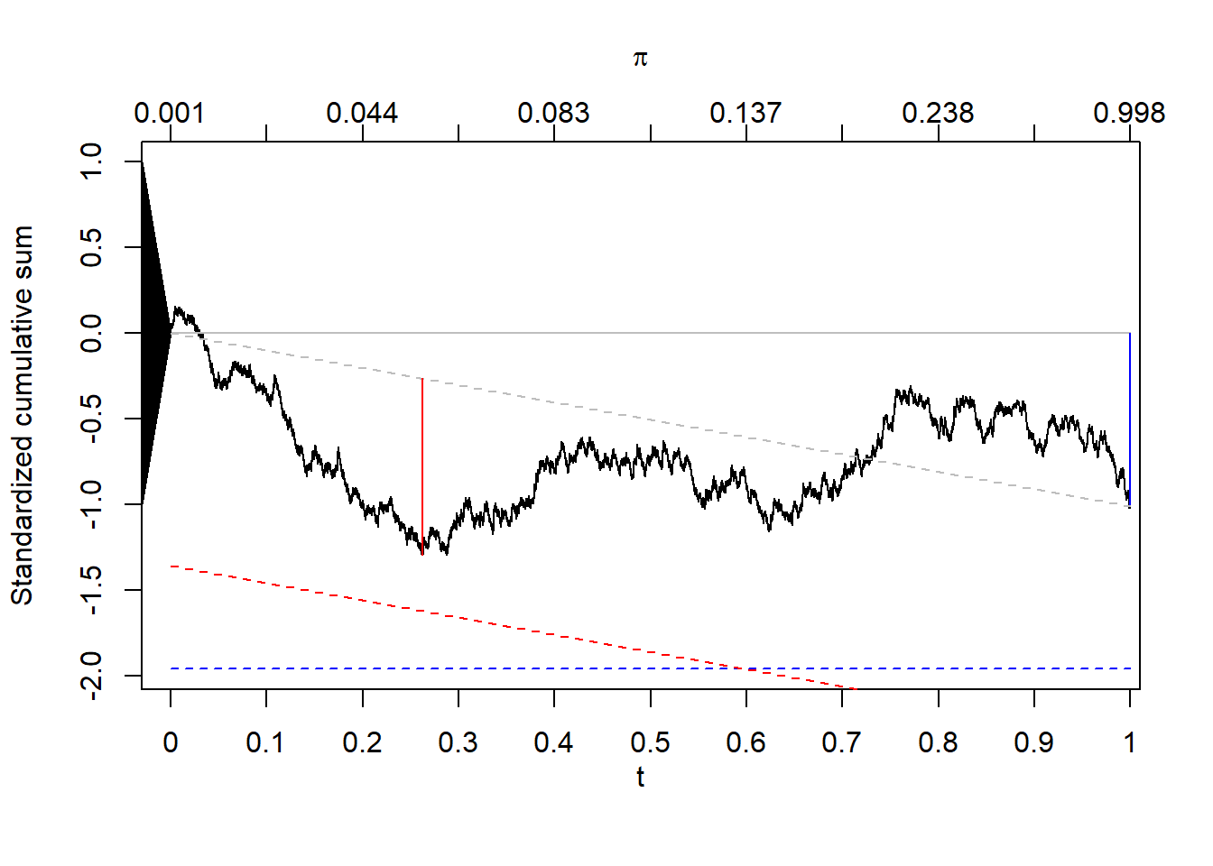
Figure 5 – panells(a) and (b) are the calibration plots of the small-sample model. The model seems to be making optimistic predictions: underestimating the risk among low/medium risk groups and overestimating it among high-risk groups. This is clearer in the partial sum plot (panels (c) and (d)), which shows an inverse U-shape that is typical of optimistic predictions. Again, the Brownian motion and bridge tests are shown on the graph in panels (c) and (d), respectively. was , corresponding to the test statistic () of and a p-value of . Maximum cumulative prediction error occurred at (). This is an estimation of the location () where the calibration function crosses the identity line. Around this point, predictions are calibrated. For individuals with predicted risk above , the model overestimates the risk by an average of (note the downward slope of the partial sum on the right side of the vertical red line in the middle panel). For others, it underestimated the risk by an average of . Bridge test results are shown in panel (d). Mean calibration was ; the Z-score for mean calibration was (p=), while was (p). The unified p-value was , clearly indicating miscalibration of this prediction model.
 |
| (a) Calibration plot (binned) |
 |
| (b) Calibration plot (smoothed) |
 |
| (c) Cumulative calibration plot (with Brownian motion test) |
 |
| (d) Cumulative calibration plot (with Brownian bridge test) |
Regression coefficients:
Discussion
In this work, we built on recently proposed non-parametric methods for the assessment of moderate calibration for models for binary outcomes. We provided suggestions on visual and statistical assessment of model calibration on the partial sum domain, proposed a novel non-parametric test, and evaluated its performance against another recently proposed test. A major advantage of these methods is no requirements for binning or smoothing of observations. Our main innovation was a stochastic process representation of the partial sum of prediction errors yielding weak convergence to standard Brownian motion. This in turn enabled us to propose a unified ‘bridge’ test of moderate calibration based on two asymptotically independent test statistics. These developments are implemented as the R package cumulcalib[24].
Our simulations point towards the higher power of the (Brownian) bridge test over the recently proposed Brownian motion test. This is not surprising as the bridge test evaluates the behavior of the underlying stochastic process in two independent ways, thus having more opportunities for identifying miscalibration. However, the bridge test also has other interesting properties. Asymptotically, follows the Kolmogorov distribution, which is ubiquitously implemented as part of the Kolmogorov-Smirnov test. The joint inference on mean and moderate calibration is also of particular relevance in clinical prediction modeling, as oftentimes mean calibration is of independent relevance and is the very first step in examining model calibration [4]. As mean calibration is a necessary condition for moderate calibration, the joint inference helps control the overall error rate of inference on calibration. We used Fisher’s method for generating a unified p-value due to its optimality properties [22]. One can also use alternative methods for retaining an overall familywise error, such as Bonferroni’s correction for each component of the test.
Our focus in this work was to propose inferential methods and evaluate their performance. However, we do not suggest inattentive use of p-values for making true / false conclusions at an arbitrary significance level on whether a model has good calibration in a population. Inferential methods quantify the compatibility of data with the null hypothesis (moderate calibration in this case), and as such complement the existing visual and numerical assessments of miscalibration. As mentioned earlier, evaluation of calibration on the partial sum domain also results in ‘distance’ metrics (e.g., or ECCE-MAD as referred to by Arrieta-Ibarra et al. [16]), similar to metrics such as Emax and ICI for calibration plots, with convergence to a finite value that is affected by the degree of miscalibration. can thus be used in a similar fashion to ICI and Emax, with the added benefit that its estimation does not require any tuning parameters. However, there are situations where one can reasonably expect that the model is calibrated, and thus hypothesis-testing becomes particularity relevant. An example is when the target population is known to be identical or very close to the development population (e.g., another random sample from the same population, or different study sites participating in a clinical trial with a strict protocol). Another relevant context is after a model is recalibrated in a new sample. Here, it is justified to expect that the revised model can provide calibrated predictions, and has a plausible chance of being true. Strictly speaking, using the same data to revise the model and evaluate its performance will result in violation of the assumption underlying the proposed tests (that the predicted risks are fixed quantities). Nevertheless, as long as the degrees of freedom used in the model updating process is small (e.g., changing the intercept, rather than re-estimating coefficients [33]), the suggested inference procedures would still provide useful insight. Indeed, this is a typical approximation underlying many GOF tests that follow model fitting. Interestingly, this is one instance where the test can be used in isolation: maximum likelihood estimation of generalized linear models (e.g., logistic regression) guarantees that the average of predicted and observed risks will be equal. In such instances, by the estimation process, and thus can be used in isolation, to avoid loss of statistical power for testing another component of the null hypothesis. Rejection of the null hypothesis in this case would indicate the need to modify the linear component (e.g., adding interaction terms) or the link function. In this sense, the bridge test acts as a GOF test for logistic regression.
There are several areas for future research. The weak convergence of the random walk to Brownian motion opens the door for possibly more powerful tests. We identified two aspects of the stochastic process that provided independent opportunities for examining moderate calibration, but one can expand this logic towards comparing multiple aspects. Examples of possible attributes include minimum, maximum, range, or integrated square value of the scaled partial sum process. An important extension of this method would be for other types of outcome, including survival outcomes (as proposed, for example, for ICI [34]). To what extent small sample correction will improve the approximation of the Kolmogorov distribution to that of the bridge test statistic can be investigated (and similar small-sample corrections can be devised for the Brownian motion test). The finite sample performance of the distance metrics based on partial sum of prediction errors versus metrics based on the calibration plots should be investigated.
Conclusion
Non-parametric approaches based on partial sums of prediction errors lead to visual, numerical, and inferential tools that do not require any grouping or smoothing of data, and thus enable objective, unequivocal, and reproducible assessments. Simulations show that the proposed bridge test for moderate calibration has comparatively high power in detecting miscalibration. We recommend such assessments to accompany conventional tools (such as calibration plots and distance metrics) to provide a more complete picture of the calibration of a risk prediction model in a target population.
References
- Van Calster and Vickers [2015] Ben Van Calster and Andrew J. Vickers. Calibration of risk prediction models: impact on decision-analytic performance. Medical Decision Making: An International Journal of the Society for Medical Decision Making, 35(2):162–169, 2 2015. ISSN 1552-681X. doi: 10.1177/0272989X14547233. PMID: 25155798.
- Van Calster et al. [2019] Ben Van Calster, David J. McLernon, Maarten Van Smeden, Laure Wynants, Ewout W. Steyerberg, Topic Group ’Evaluating diagnostic tests, and prediction models’ of the STRATOS initiative. Calibration: the achilles heel of predictive analytics. BMC medicine, 17(1):230, 12 2019. ISSN 1741-7015. doi: 10.1186/s12916-019-1466-7. PMID: 31842878 PMCID: PMC6912996.
- Van Calster et al. [2016] Ben Van Calster, Daan Nieboer, Yvonne Vergouwe, Bavo De Cock, Michael J. Pencina, and Ewout W. Steyerberg. A calibration hierarchy for risk models was defined: from utopia to empirical data. Journal of Clinical Epidemiology, 74:167–176, 2016. ISSN 1878-5921. doi: 10.1016/j.jclinepi.2015.12.005. PMID: 26772608.
- Steyerberg and Vergouwe [2014] Ewout W. Steyerberg and Yvonne Vergouwe. Towards better clinical prediction models: seven steps for development and an abcd for validation. European Heart Journal, 35(29):1925–1931, 8 2014. ISSN 1522-9645. doi: 10.1093/eurheartj/ehu207. PMID: 24898551 PMCID: PMC4155437.
- Van Hoorde et al. [2015] K. Van Hoorde, S. Van Huffel, D. Timmerman, T. Bourne, and B. Van Calster. A spline-based tool to assess and visualize the calibration of multiclass risk predictions. J Biomed Inform, 54:283–293, April 2015. ISSN 1532-0480. doi: 10.1016/j.jbi.2014.12.016.
- Harrell [2015] Frank E. Harrell. Regression modeling strategies: with applications to linear models, logistic and ordinal regression, and survival analysis. Springer series in statistics. Springer, Cham Heidelberg New York, second edition edition, 2015. ISBN 978-3-319-33039-6. OCLC: 922304565.
- Austin and Steyerberg [2019] Peter C. Austin and Ewout W. Steyerberg. The integrated calibration index (ici) and related metrics for quantifying the calibration of logistic regression models. Statistics in Medicine, 38(21):4051–4065, 9 2019. ISSN 1097-0258. doi: 10.1002/sim.8281. PMID: 31270850.
- Hosmer and Lemesbow [1980] David W. Hosmer and Stanley Lemesbow. Goodness of fit tests for the multiple logistic regression model. Communications in Statistics - Theory and Methods, 9(10):1043–1069, 1980. ISSN 0361-0926. doi: 10.1080/03610928008827941.
- Hosmer et al. [1997] David W. Hosmer, T. Hosmer, S. Le Cessie, and S. Lemeshow. A comparison of goodness-of-fit tests for the logistic regression model. Statistics in Medicine, 16(9):965–980, 5 1997. ISSN 0277-6715. doi: https://doi.org/10.1002/(sici)1097-0258(19970515)16:9\%3C965::aid-sim509\%3E3.0.co;2-o. PMID: 9160492.
- Sadatsafavi et al. [2022] Mohsen Sadatsafavi, Paramita Saha-Chaudhuri, and John Petkau. Model-based roc curve: Examining the effect of case mix and model calibration on the roc plot. Med Decis Making, 42(4):487–499, 5 2022. ISSN 1552-681X 0272-989X. doi: 10.1177/0272989X211050909. PMID: 34657518 PMCID: PMC9005838.
- Allison [2014] Paul Allison. Measures of fit for logistic regression. Technical report, SAS, 2014. URL https://support.sas.com/resources/papers/proceedings14/1485-2014.pdf. [Online; accessed 2020-11-12].
- Delgado [1993] Miguel A. Delgado. Testing the equality of nonparametric regression curves. Statistics & Probability Letters, 17(3):199–204, 6 1993. ISSN 01677152. doi: 10.1016/0167-7152(93)90167-H.
- Diebolt [1995] Jean Diebolt. A nonparametric test for the regression function: Asymptotic theory. Journal of Statistical Planning and Inference, 44(1):1–17, 3 1995. ISSN 03783758. doi: 10.1016/0378-3758(94)00045-W.
- Stute [1997] Winfried Stute. Nonparametric model checks for regression. The Annals of Statistics, 25(2), 4 1997. ISSN 0090-5364. doi: 10.1214/aos/1031833666. URL https://projecteuclid.org/journals/annals-of-statistics/volume-25/issue-2/Nonparametric-model-checks-for-regression/10.1214/aos/1031833666.full. [Online; accessed 2023-06-23].
- Tygert [2020] Mark Tygert. Plots of the cumulative differences between observed and expected values of ordered bernoulli variates. arxiv, 2020. doi: 10.48550/ARXIV.2006.02504. URL https://arxiv.org/abs/2006.02504. publisher: arXiv version: 3.
- Arrieta-Ibarra et al. [2022] Imanol Arrieta-Ibarra, Paman Gujral, Jonathan Tannen, Mark Tygert, and Cherie Xu. Metrics of calibration for probabilistic predictions. Journal of machine learning research, 23, 2022. doi: 10.48550/ARXIV.2205.09680. URL https://dl.acm.org/doi/10.5555/3586589.3586940.
- Borodin and Salminen [1996] A. N. Borodin and Paavo Salminen. Handbook of Brownian motion: facts and formulae. Probability and its applications. Birkhäuser Verlag, Basel ; Boston, 1996. ISBN 978-3-7643-5463-3.
- Lindeberg [1922] J. W. Lindeberg. Eine neue herleitung des exponentialgesetzes in der wahrscheinlichkeitsrechnung. Mathematische Zeitschrift, 15(1):211–225, 12 1922. ISSN 0025-5874, 1432-1823. doi: 10.1007/BF01494395.
- Brown [1971] B. M. Brown. Martingale central limit theorems. The Annals of Mathematical Statistics, 42(1):59–66, 2 1971. ISSN 0003-4851. doi: 10.1214/aoms/1177693494.
- Chow [2009] Winston C. Chow. Brownian bridge. WIREs Computational Statistics, 1(3):325–332, 11 2009. ISSN 1939-5108, 1939-0068. doi: 10.1002/wics.38.
- Marsaglia et al. [2003] George Marsaglia, Wai Wan Tsang, and Jingbo Wang. Evaluating kolmogorov’s distribution. Journal of Statistical Software, 8(18), 2003. ISSN 1548-7660. doi: 10.18637/jss.v008.i18. URL http://www.jstatsoft.org/v08/i18/. [Online; accessed 2023-06-09].
- Littell and Folks [1971] Ramon C. Littell and J. Leroy Folks. Asymptotic optimality of fisher’s method of combining independent tests. Journal of the American Statistical Association, 66(336):802–806, 12 1971. ISSN 0162-1459, 1537-274X. doi: 10.1080/01621459.1971.10482347.
- R Core Team [2019] R Core Team. R: A Language and Environment for Statistical Computing. R Foundation for Statistical Computing, Vienna, Austria, 2019. URL https://www.R-project.org/.
- Sadatsafavi [2024] Mohsen Sadatsafavi. Cumulcalib: cumulative calibration assessment (development version) - https://github.com/resplab/cumulcalib. github.com, 2024. URL https://github.com/resplab/cumulcalib.
- Miller [2018] Curtis Miller. CPAT: Change Point Analysis Tests. CRAN, 2018. URL https://CRAN.R-project.org/package=CPAT.
- Vrbik [2020] Jan Vrbik. Deriving cdf of kolmogorov-smirnov test statistic. Applied Mathematics, 11(03):227–246, 2020. ISSN 2152-7385, 2152-7393. doi: 10.4236/am.2020.113018.
- Morris et al. [2019] Tim P. Morris, Ian R. White, and Michael J. Crowther. Using simulation studies to evaluate statistical methods. Statistics in Medicine, 38(11):2074–2102, 5 2019. ISSN 1097-0258. doi: 10.1002/sim.8086. PMID: 30652356 PMCID: PMC6492164.
- GUSTO investigators [1993] GUSTO investigators. An international randomized trial comparing four thrombolytic strategies for acute myocardial infarction. The New England Journal of Medicine, 329(10):673–682, 9 1993. ISSN 0028-4793. doi: 10.1056/NEJM199309023291001. PMID: 8204123.
- Ennis et al. [1998] M. Ennis, G. Hinton, D. Naylor, M. Revow, and R. Tibshirani. A comparison of statistical learning methods on the gusto database. Statistics in Medicine, 17(21):2501–2508, 11 1998. ISSN 0277-6715. doi: 10.1002/(SICI)1097-0258(19981115)17:21<2501::AID-SIM938>3.0.CO;2-M. PMID: 9819841.
- Steyerberg et al. [2005a] Ewout W. Steyerberg, Marinus J. C. Eijkemans, Eric Boersma, and J. Dik F. Habbema. Applicability of clinical prediction models in acute myocardial infarction: a comparison of traditional and empirical bayes adjustment methods. American Heart Journal, 150(5):920, 11 2005a. ISSN 1097-6744. doi: 10.1016/j.ahj.2005.07.008. PMID: 16290963.
- Steyerberg et al. [2005b] Ewout W. Steyerberg, Marinus J. C. Eijkemans, Eric Boersma, and J. D. F. Habbema. Equally valid models gave divergent predictions for mortality in acute myocardial infarction patients in a comparison of logistic [corrected] regression models. Journal of Clinical Epidemiology, 58(4):383–390, 4 2005b. ISSN 0895-4356. doi: 10.1016/j.jclinepi.2004.07.008. PMID: 15862724.
- Sadatsafavi et al. [2023] Mohsen Sadatsafavi, Tae Yoon Lee, Laure Wynants, Andrew J. Vickers, and Paul Gustafson. Value-of-Information Analysis for External Validation of Risk Prediction Models. Medical Decision Making: An International Journal of the Society for Medical Decision Making, 43(5):564–575, July 2023. ISSN 1552-681X. doi: 10.1177/0272989X231178317.
- Steyerberg et al. [2004] Ewout W. Steyerberg, Gerard J. J. M. Borsboom, Hans C. Van Houwelingen, Marinus J. C. Eijkemans, and J. Dik F. Habbema. Validation and updating of predictive logistic regression models: a study on sample size and shrinkage. Statistics in Medicine, 23(16):2567–2586, 8 2004. ISSN 0277-6715. doi: 10.1002/sim.1844. PMID: 15287085.
- Austin et al. [2022] Peter C. Austin, Hein Putter, Daniele Giardiello, and David Van Klaveren. Graphical calibration curves and the integrated calibration index (ici) for competing risk models. Diagnostic and Prognostic Research, 6(1):2, 1 2022. ISSN 2397-7523. doi: 10.1186/s41512-021-00114-6. PMID: 35039069 PMCID: PMC8762819.
Appendix A: Asymptotic sufficiency of the bridge test for moderate calibration
Let be the calibration error at predicted risk . The model is moderately calibrated if . Let be the cumulative distribution function of the infinite population of predicted risks. The argument is for when is strictly monotone in [0,1].
In the general case where the null hypothesis is not known to hold, the random walk constructed in the main text might have a non-zero expected value (drift). Indeed, as , at time , , where , and is the unique solution for in . Correspondingly, the bridged random walk will have an expected value of:
The second component of the bridge test () demands that converges to a Brownian bridge, thus requiring it to have zero expected value everywhere:
Given the 1:1 relation between and and the monotonicity of , we can map this equality to the domain:
Taking the first derivative with respect to and re-arranging terms, we have:
The right-hand side is a constant so the solutions are of the form , and it is immediately obvious that any provides a valid solution. On the other hand, the hypothesis for mean calibration, , demands that . Therefore, the two null hypotheses together impose , which can only hold for , which implies moderate calibration.
Appendix B: R code for the implementation of the bridge test
We use birth weight data in the MASS package and an exemplary model for predicting low birth weight. Below, as a generic implementation we use the ks.test implementation of Kolmogorov CDF by creating a vector of n (=100) observation whose empirical CDF has distance B*/sqrt(n) from the CDF of the standard uniform distribution, such that when multiplied by sqrt(n) as part of the KS test it generates the desired metric. In R, one can request asymptotic test via ks.test() with exact=F argument. Of note, the /pKolmogorov() function in the cumulcalib package provides a direct implementation of this test.
library(MASS)
data("birthwt")
pi <- 1/(1+exp(-(2.15-0.050*birthwt$age-0.015*birthwt$lwt))) #The model

#Ordering predictions (and responses) from smallest to largest pi
o <- order(pi)
pi <- pi[o]
Y <- birthwt$low[o] #Outcome is low birth weight (1 v 0)

#Constructing the {S} process
T <- sum(pi*(1-pi))
t <- cumsum(pi*(1-pi))/T
S <- cumsum(Y-pi)/sqrt(T)

plot(t,S, type=’l’)

Sn <- S[length(S)] #This is Sn, the first component of the bridge test
pA <- 2*pnorm(-abs(Sn)) #p-value for first component of H0

Bstar <- max(abs(S-t*Sn)) #This is B*, the second component of the bridge test
d <- Bstar/10
X <- seq(from=0, to=1-d, length.out=100)
pB <- ks.test(X, punif, exact=F)$p.value #p-value for second component of H0

#Fisher’s method for generating a unified p-value
p <- 1-pchisq(-2*(log(pA)+log(pB)),4) #0.8381805