Non-myopic Beam Scheduling for Multiple Smart Target Tracking in Phased Array Radar Network

We consider $N$ smart targets labeled by $n=1,2,\ldots,N$ and a radar network consisting of $K<N$ phased array radars, as illustrated in Fig. 1. In Fig. 1, targets 1 and $N$ will likely change their dynamics models in response to radar tracking, while target 2 will be likely to maintain its dynamics model. All radars are synchronized to operate over time slots $t=0,1,\ldots$. The radar network centrally steers beams to track at most $K$ targets at each time, as one radar beam can be only assigned to one target in a time slot.

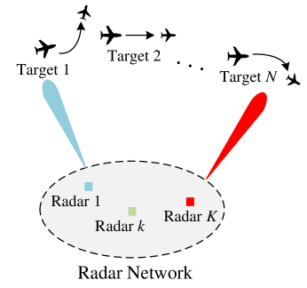
We assume that radars detect targets with unit probability. Denote the kinematic state of target $n$ at time $t$ by $\bm{x}_{n,t}\in\mathbb{R}^{L}$. Targets follow independent linear dynamics. Meanwhile, they are smart, that is, they react to radar radiation by switching between $M$ dynamics models, labeled by $m=1,2,\ldots,M$, e.g., CV, CA, CT, etc. Target $n$’s dynamics under model $m$ is

In (1), $\bm{F}_{n}^{m}$ is the state transition matrix, and $\bm{w}_{n,t}^{m}$ is process noise with mean being zero and covariance matrix being $\bm{\mathrm{Q}}_{n}^{m}$. We assume that $\bm{\mathrm{Q}}_{n}^{m}=q_{n}^{m}\bm{\mathrm{Q}}_{n}$ for a covariance matrix $\bm{\mathrm{Q}}_{n}$, where $0<q_{n}^{1}<q_{n}^{2}<\cdots<q_{n}^{M}$ and $m=1$ corresponds to the CV model, so the uncertainty of the dynamics model increases with $m$.

At each time $t$, we use a binary variable $a_{n,t}\in\left\{0,1\right\}$ to denote the tracking action imposed on target $n$. Let $a_{n,t}=0$ if target $n$ is not tracked. Conversely, when $a_{n,t}=1$, the target is actively tracked, and a measurement $\bm{y}_{n,t}$ is acquired following the subsequent measurement equation,

where $\bm{\mathrm{H}}_{n}$ is the measurement matrix, and $\bm{v}_{n,t}$ is a zero-mean Gaussian white noise with covariance matrix $\bm{\mathrm{R}}_{n}$.

Targets are assumed to change their dynamics models depending only on whether they are being tracked. After action $a_{n}$ is applied on target $n$ at each time, its dynamics model is randomly drawn to be $m$ with probability $u_{n}^{a_{n},m}$, for $m=1,\ldots,M$. We write $\bm{\mathrm{U}}_{n}\triangleq\left[\bm{u}_{n}^{0},\bm{u}_{n}^{1}\right]$, where $\bm{u}_{n}^{a_{n}}=\left[u_{n}^{a_{n},1},\ldots,u_{n}^{a_{n},M}\right]^{\prime}$ and $(\cdot)^{\prime}$ is the transpose operator. We assume that $u_{n}^{0,1}>u_{n}^{0,m}$, $m=2,3,\ldots,M$, so targets that are not being tracked are more likely to move into model $m=1$ (CV). We further assume that $u_{n}^{1,1}<u_{n}^{1,m}$ for $m=2,3,\ldots,M$, so targets that are being tracked are less likely to move into model $m=1$.

Consequently, the smart targets are characterized by the dynamics model probability matrix, and the states $\bm{x}$ of the targets are affected not only by the CV model but also by the other dynamics models.

Target TECs evolve based on the Kalman filter [52]. Denote by ${\mathbf{P}}_{n,t}$ the TEC of target $n$ at the beginning of time slot $t$. Starting from the initial TEC ${\mathbf{P}}_{n,0}$, ${\mathbf{P}}_{n,t}$ is recursively updated over time slots $t\geq 1$ being conditioned by the chosen actions, taking into account the dynamics models, as follows.

If the target is tracked at time $t-1$ ($a_{n,t-1}=1$), then

where

and $\bm{\mathrm{I}}$ is the $L\times L$ identity matrix.

If the target is not tracked at time $t-1$ ($a_{n,t-1}=0$), then

Note that the TEC update recursion given by (3)–(7) is deterministic. It follows that action $a_{n,t-1}$ updates the TEC ${\bm{\mathrm{P}}}_{n,t}$ through sum-weighted method based on the model probability vector $\bm{u}_{n}^{a_{n,t-1}}$. When $a_{n,t-1}=1$, the target $n$ maneuvers with higher probability $u_{n}^{1,m}$, $m=2,3,\ldots,M$ than CV with lower probability $u_{n}^{1,1}$. It leads to a larger determinant of TEC state ${\bm{\mathrm{P}}}_{n,t}$ than that of $\hat{\bm{\mathrm{P}}}_{n,t}^{1,1}$ solely calculated by CV model. If $a_{n,t-1}=0$, then, since $q_{n}^{1}<q_{n}^{m}$, $m=2,3,\ldots,M$, with larger $u_{n}^{0,1}$ in (7), the determinant of TEC state ${\bm{\mathrm{P}}}_{n,t}$ will be smaller than that with probability $\bm{u}_{n}^{1}$.

We next formulate the optimal beam scheduling problem for $K$ radars and $N$ smart targets as an infinite-horizon discrete-time RMABP, aiming to achieve the optimal dynamic selection of $K$ out of $N$ binary-action projects. For such a purpose, we identify a target with a project, which can be operated under the active action (track the target) and the passive action (do not track it). We take as the state of project $n=1,\ldots,N$ the corresponding target’s TEC, $\mathbf{P}_{n,t}$, which moves over the state space $\mathbb{S}_{++}^{L}$ of symmetric positive definite $L\times L$ matrices, according to Kalman filter dynamics as shown in Section II-C.

For target $n$ at time $t$, the immediate cost caused by imposing action $a_{n,t}$ is defined as

where $\mathrm{tr}(\cdot)$ denotes the trace of a matrix, $d_{n}\geq 0$ is the target’s weight, which is used to model the importance of targets, and $h_{n}\geq 0$ is a measurement cost.

The radar network selects at most $K$ out of $N$ smart targets to track in each time slot $t$. We consider that each radar can only steer one beam to track one target at each time, which is formulated as the constraint

Given the joint model probabilities $\bm{\mathbb{U}}=(\bm{\mathrm{U}}_{n})_{n=1}^{N}$ and a TEC state at the beginning $\mathbf{\mathbb{P}}_{0}=(\mathbf{P}_{n,0})_{n=1}^{N}$, we consider the dynamic optimization problem with discounted cost over an infinite time horizon.

where $0<\beta<1$ is the discount factor, $\mathrm{E}_{\mathbf{\mathbb{P}}_{0}}^{\bm{\pi}}[\cdot]$ is expectation under policy $\bm{\mathrm{\pi}}$ conditioned on the initial state $\mathbf{\mathbb{P}}_{0}$, and denote by $\Pi(K)$ the set of stationary scheduling policies that satisfy (9). We denote by $V^{*}\left(\mathbf{\mathbb{P}}_{0}\right)$ the optimal cost of problem (10).

To obtain a relaxed version of problem (10), we replace the sample-path constraint (9) by the following constraint,

Now, consistently with the above notation ${\Pi}(K)$, let ${\Pi}(N)$ represent the set of stationary scheduling policies capable of activating any quantity of projects (tracking any number of targets) at each time. Then, a relaxation of problem (10) is as follows.

Therefore, the minimum cost $V^{\textup{R}}(\mathbf{\mathbb{P}}_{0})$ derived from problem (12) establishes a lower bound on $V^{*}(\mathbf{\mathbb{P}}_{0})$.

Attach now a Lagrange multiplier $\lambda\geq 0$ to the aggregate constraint (11). The Lagrangian relaxation applied to (12) is

Given a $\lambda\geq 0$, the optimal value of the Lagrangian relaxation, denoted as $V^{\textup{L}}(\mathbf{\mathbb{P}}_{0};\lambda)$, serves as a lower bound for $V^{\textup{R}}(\mathbf{\mathbb{P}}_{0})$.

If we search for an optimal Lagrange multiplier $\lambda^{*}(\mathbf{\mathbb{P}}_{0})$ based on the Lagrangian relaxation, the best lower bound for $V^{\textup{R}}(\mathbf{\mathbb{P}}_{0})$ is obtained. This defines the dual problem of (12):

Problem (13) can be decomposed into $N$ single-target independent subproblems given by

In (15), $\Pi^{n}$ is the set of stationary scheduling policies corresponding to target $n$. Here, multiplier $\lambda$ has the economic interpretation of an additional tracking cost.

In the one-dimensional case with real-valued state space for a single bandit process, $V^{\textup{D}}\left((P_{n,0})_{n=1}^{N}\right)$ can be calculated through the value iteration approach [53]. In general, consider the lower bound $V^{\textup{D}}(\mathbf{\mathbb{P}}_{0})$ in (14) which is the optimal value of the Lagrangian dual problem. Recall that we aim to minimize the expected total discounted (ETD) cost. Based on the Bellman equation, we firstly derive the optimal value function for the process $\{\mathbf{P}_{n,t},t=0,1,\ldots\}$ of target $n$ in (15). Given the Lagrange multiplier $\lambda$, we obtain

Subsequently given the Lagrange multiplier $\lambda$ in (13), we can derive the multitarget optimal value function $L^{\lambda,*}\left(\mathbf{\mathbb{P}}_{t}\right)$ and substitute (16) into it, as given by

where

representing the next-slot joint target states.

Based on the established value function and a given $\lambda$, we establish the $k$-th iteration of value function $v^{\lambda}_{n,k}\left(\mathbf{P}_{n,t}\right)$ as

Then, we use the value iteration approach to continue the iterative process over the state space until convergence of values on diverse joint state $\mathbf{\mathbb{P}}_{t}$. Finally, we obtain the optimal value $v^{\lambda,*}_{n}\left(\mathbf{P}_{n,t}\right)$ in (16) and derive $L^{\lambda,*}\left(\mathbf{\mathbb{P}}_{t}\right)$ in (17). Given the initial joint state $\mathbf{\mathbb{P}}_{0}$ and a given $\lambda$, the minimum cost $V^{\textup{L}}(\mathbf{\mathbb{P}}_{0};\lambda)$ can be computed by $L^{\lambda,*}\left(\mathbf{\mathbb{P}}_{0}\right)$. The lower bound $V^{\textup{D}}\left(\mathbf{\mathbb{P}}_{0}\right)$ of the dual problem in (14) can be computed by searching a $\lambda\in(0,\infty)$ to satisfy

Above all, we regard the lower bound of problem (14) as the optimal cost of the original problem (10) to further calculate the suboptimality gap of policies and numerically analyze the near optimality of the Whittle index policy, given a constant ratio $\xi=K/N$.

Consider now the following structural property of subproblems (15), referred to as indexability in [28], which we formulate next as in [47, Section 3.2]. Note that target $n$’s subproblem (15) is indexable if there exists an index $\lambda_{n}^{*}\colon\mathbb{S}_{++}^{L}\to\mathbb{R}$ that characterizes its optimal policies, as follows: for any $\lambda\in\mathbb{R}$, when the target is in state $\mathbf{P}_{n}$, $\lambda_{n}^{*}(\mathbf{P}_{n})>\lambda$ ($\lambda_{n}^{*}(\mathbf{P}_{n})\leq\lambda$) is necessary and sufficient conditions for that taking action $a_{n}=1$ ($a_{n}=0$) is optimal.

If each subproblem were indexable, the Whittle index policy would be to track up to $K$ out of the $N$ targets with larger index values, among those with nonnegative indices. If the current index of a target is negative, it is not tracked.

Yet, at present it is unknown whether restless projects with multi-dimensional Kalman filter dynamics such as those above are indexable, even for a single dynamics model ($M=1$). Indexability has only been established (in [49]) for the special case of target tracking with scalar Kalman filter dynamics and a single dynamics model, by applying the PCL-indexability approach for real-state projects in [43].

We next outline the PCL-indexability approach for real-state restless bandit projects as it applies to the present model (so $L=1$). In the sequel we pay attention to the MP index of a single target with multiple dynamics models as described above, and drop the subscript $n$ from notations.

Starting from an initial state $P_{0}=P\in\mathbb{S}_{++}\triangleq(0,\infty)$, for a policy $\pi$, define the cost metric

which gives the ETD cost, where $P$ is the target’s tracking error variance (TEV) state.

The work metric is defined as

The subproblem (15) can be reformulated as

The indexability of subproblem (23) is studied under deterministic stationary policies and threshold policies. Deterministic stationary policies are represented as (Borel measurable) subsets of TEV states, where the corresponding target is tracked. We will employ an active set denoted as $B\subseteq\mathbb{S}_{++}$ to characterize the $B$-active policy. In particular, for any given threshold level $z\in\bar{\mathbb{S}}\triangleq\mathbb{S}_{{++}}\cup\{-\infty,\infty\}$, we will designate this as the $z$-threshold policy. This means that, for a target in TEV state $P$, if $P>z$, the target is tracked; otherwise, it is not tracked. Therefore, a $z$-threshold policy has active set $B(z)\triangleq\{P\in\mathbb{S}_{++}:P>z\}$. It is clear that, if $0<z<\infty$, then $B(z)=(z,\infty)$; if $z\leq 0$, then $B(z)=\mathbb{S}_{++}$; and if $z=\infty$, then $B(z)=\emptyset$. We shall denote the corresponding cost and work metrics in (21) and (22) by $F(P,z)$ and $G(P,z)$, respectively.

Given a threshold $z$, the cost and work metrics are characterized by the functional equations.

and

In practice, such metrics can be approximately computed by a value-iteration scheme with a finite truncated time horizon $\tau$, as discussed in [43, Section 11].

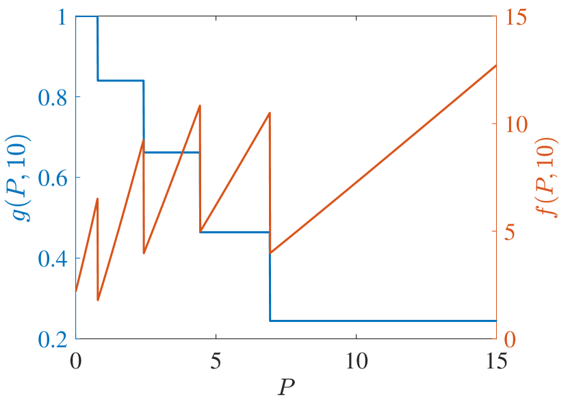
Next, we represent as $\langle a,z\rangle$ the policy that executes action $a$ at time $t=0$ and subsequently follows the $z$-threshold policy from $t=1$ onwards. Accordingly, we introduce the corresponding marginal metrics for the previously discussed measures. Specifically, we define the marginal cost metric $f(P,z)\triangleq F(P,\langle 0,z\rangle)-F(P,\langle 1,z\rangle)$ and the marginal work metric $g(P,z)\triangleq G(P,\langle 1,z\rangle)-G(P,\langle 0,z\rangle)$. If $g(P,z)>0$, we further define the MP metric function by

If $g(P,P)>0$ for all $P$, we define the MP index by

As in [43, Definition 7], we say that the subproblem (23) is PCL-indexable (with respect to threshold policies) if the following PCL-indexability conditions hold:

• •

  (PCLI1) $g(P,z)>0$ for every state $P$ and threshold $z$;

• •

  (PCLI2) $\mathrm{mp}^{*}(P)$ is monotone non-decreasing, continuous, and bounded below;

• •

  (PCLI3) for each $P$, the metrics $F(P,z)$, $G(P,z)$ and the index $\mathrm{mp}^{*}(P)$ are related by: for $-\infty<z_{1}<z_{2}<\infty$,

  $$F(P,z_{2})-F(P,z_{1})=\int_{(z_{1},z_{2}]}\mathrm{mp}^{*}(z)\,G(P,dz),$$

  where the right-hand side is a Lebesgue–Stieltjes integral.

The interest of the above PCL-indexability conditions lies in their applicability through the verification theorem in [43, Theorem 1], which ensures that, for a real-state project, conditions (PCLI1)–(PCLI3) above imply that the project is indexable, and the MP index $\mathrm{mp}^{*}(P)$ is its Whittle index.

This was the approach deployed in [49] to prove indexability for the special case of a single dynamics model ($M=1$). Yet, proving that conditions (PCLI1)–(PCLI3) hold for the present model with $M\geq 2$ is beyond the scope of this work. Still, we conjecture that the model satisfies such conditions, and will present partial numerical evidence supporting satisfaction of such conditions. We shall further use the MP index above as a surrogate of the Whittle index, and refer to it as the Whittle index. Note that only if it were proven that conditions (PCLI1)–(PCLI3) hold could we ensure that the MP index is indeed the Whittle index.

In the case of target dynamic states moving over in a $L$-dimensional state space $\mathbb{R}^{L}$, with $L\geq 2$, the TEC matrix indicates the tracking accuracy of the target state’s components, e.g., location and velocity. Since the TEC state is an $L\times L$ matrix, a convenient scalar measure of tracking performance is given by its trace. The application of the PCL-indexability approach for proving indexability and evaluating the Whittle index in such a case remains an open problem, even in the case of single target dynamics ($M=1$). This section leverages the past success of the PCL-indexability and extends a new heuristic approach to define an MP index for the multi-dimensional case.

In particular, we define the cost metric $F(\mathbf{P},\pi)$ and the work metric $G(\mathbf{P},\pi)$ by replacing the one-dimensional $P$ in (21) and (22) with the multi-dimensional $\mathbf{P}$. The target’s optimal tracking subproblem (15) becomes

We need to define the meaning of threshold policies in the present setting. For such a purpose, we shall consider that the $z$-threshold policy tracks the target in state $\mathbf{P}$ if and only if $\mathrm{tr}(\mathbf{P})/{L}>z$. Then, the corresponding cost metric $F(\mathbf{P},z)$ and work metric $G(\mathbf{P},z)$ are the unique solutions to the following functional equations:

Again, we can approximate such solutions through a value-iteration approach using a truncated time horizon $\tau$.

Now, similar to the scalar case above, we define the marginal cost metric $f(\mathbf{P},z)$, the marginal work metric $g(\mathbf{P},z)$, and the MP metric

provided that $g(\mathbf{P},z)>0$.

The corresponding MP index is defined by

provided that $g(\mathbf{P},\mathrm{tr}(\mathbf{P})/L)>0$ for all $\mathbf{P}$.

However, there is currently no theory supporting any relation of the index $\mathrm{mp}^{*}(\mathbf{P})$ with the Whittle index in the multi-dimensional case, assuming that both are well defined. Still, we will discuss in Section IV the results of a simulation study on the performance of the index policy based on the heuristic MP index $\mathrm{mp}^{*}(\mathbf{P})$.

In Sections III-D and III-E, we discussed the MP-based indices for a bandit process with real-valued and multi-dimensional state spaces, respectively. In general, the MP-based index policy prioritizes tracking specific targets based on their state-dependent MP indices, regardless of the dimensions of the state, in descending order. The pseudo-code of implementing the index policy with given indices is provided in Algorithm 1, which is applicable to both cases with one-dimensional and multi-dimensional state spaces.

For the case with real-valued bandit states, the complexity for computing the indices in (32) is only linear in the number of targets $N$ and the truncated time $\tau$. Nonetheless, for the case with multi-dimensional state space for each bandit process, the linearity does not hold in general due to the complex matrix operations in (3) and (7).

In the Whittle index policy, the truncated time horizon $\tau$ is the recursive horizon in (29) and (30). If the actions of each target across $\tau$ time horizon are all assumed as 0, the computational complexity of (31) is $2N\tau(n_{\phi^{0}}+4)+2+1$. Otherwise, the computational complexity is $2N\tau(n_{\phi^{1}}+4)+2+1$, where $n_{\phi^{1}}$ and $n_{\phi^{0}}$ ($n_{\phi^{0}}<n_{\phi^{1}}$) represent the complexity of updating matrix states when the corresponding action variable is set to $1$ and $0$, respectively. Due to the diverse combination of actions across $\tau$ time horizon, the computational complexity of the Whittle index is less than $2N\tau(n_{\phi^{1}}+4)+2+1$. That is, we have a complexity of $O(N\tau)$.

We introduce two greedy approaches as baseline policies. One is the TEC index policy, which defines the indices by

The computational complexity of the TEC index is $O(N)$. The other prioritizes actions according to the MP indices with $\beta=0$, namely, the myopic index policy with the indices given by

The computational complexity for $\mathrm{mp}^{\text{myopic}}$ is $O(N(n_{\phi^{1}}+n_{\phi^{0}}))$. The baseline policies exhibit lower computational complexity but, in general, fail to take consideration of long future effects of the employed actions. Based on numerical results in [46, 47, 38], with appropriate $\beta$ ($\beta\leq 0.9$), the MP indices $\mathrm{mp}^{*}(\bm{P})$ (described in (32)) with truncated horizon $\tau=100$ is sufficiently close to the analytical Whittle indices, for which the computational complexity is comparable to the greedy approaches.

We start by considering the PCL-indexability conditions stated in Section III-D as they apply to scalar state targets. Recall that they are sufficient conditions for indexability (existence of the Whittle index) and further give an explicit expression of the Whittle index in the form of an MP index. Establishing analytically that the present model satisfies such conditions is beyond the scope of this work. Still, we present below a sample of numerical evidence supporting the conjecture that the model satisfies such conditions.

To test the conditions numerically, we consider targets with $M=2$ dynamics models, which we refer to as CV ($m=1$) and CT ($m=2$), and parameter values $F^{\text{CV}}=1.1$, $F^{\text{CT}}=1.3$, $Q^{\text{CV}}=1$, $Q^{\text{CT}}>Q^{\text{CV}}$, $H=1$, and $R=2$. There are no measurement costs ($h=0$) and the weight is $d=1$. We assume two types of smart targets, called reckless and cautious, where reckless targets have a higher probability of maneuvering (using the CT model) when tracked than cautious targets. Hence, the dynamics model probability matrix $\bm{\mathrm{U}}=\left[\bm{u}^{0},\bm{u}^{1}\right]$ differs with the target types. Specifically, we take

where, if target $n_{1}$ belongs to reckless targets, target $n_{2}$ belongs to cautious targets, we can obtain $u_{n_{1}}^{0,m}>u_{n_{2}}^{0,m}$ and $u_{n_{1}}^{1,m}>u_{n_{2}}^{1,m}$, $m=2,\ldots,M$.

In the following numerical experiments, the infinite series defining the metrics of interest have been approximately computed by using the truncated time horizon $\tau=100$. The discount factor is $\beta=0.9$, and the TEV state $P$ has been taken from a grid of values, each separated by a distance of $10^{-2}$.

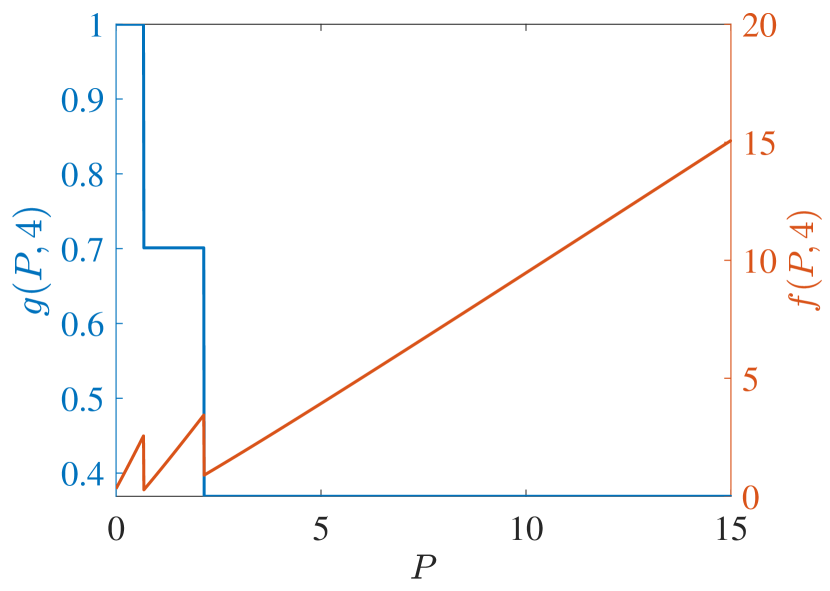
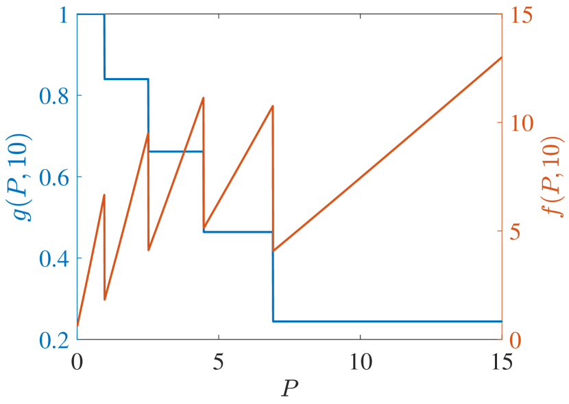
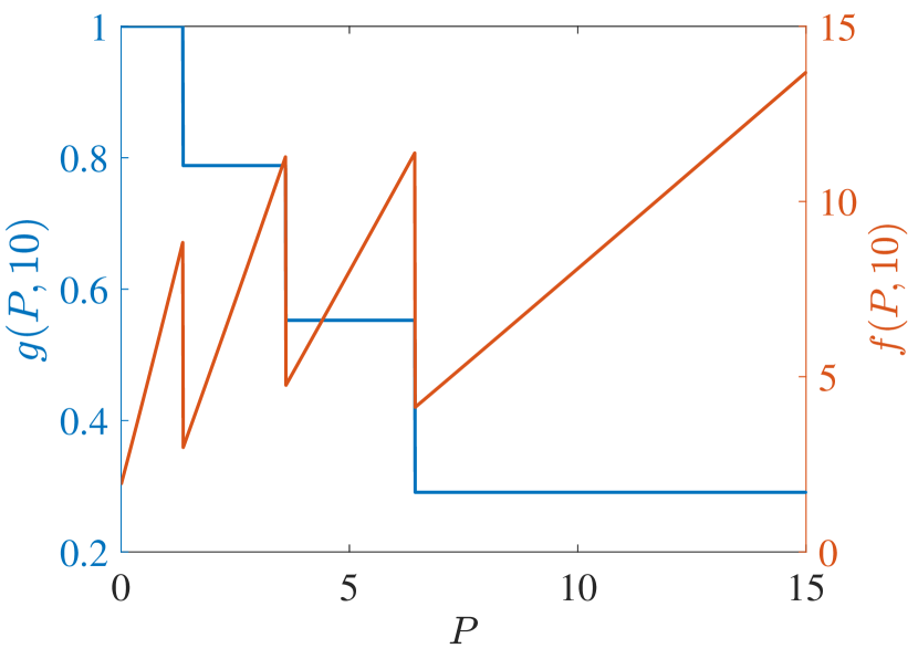
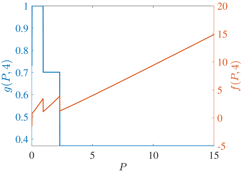
Start with PCL-indexability condition (PCLI1), namely that marginal work metric $g(P,z)$ be positive for each TEV state $P$ and threshold $z$. Figs. 2 and 3 plot both $g(P,z)$ and the marginal cost metric $f(P,z)$ against $P$ for several choices of threshold $z$ and of the $Q^{\text{CT}}$ parameter, for reckless targets and cautious targets in Fig. 2 and Fig. 3, respectively. The plots support the validity of condition (PCLI1), as $g(P,z)>0$ in each instance, a result that has been observed under other parameter choices not reported here.

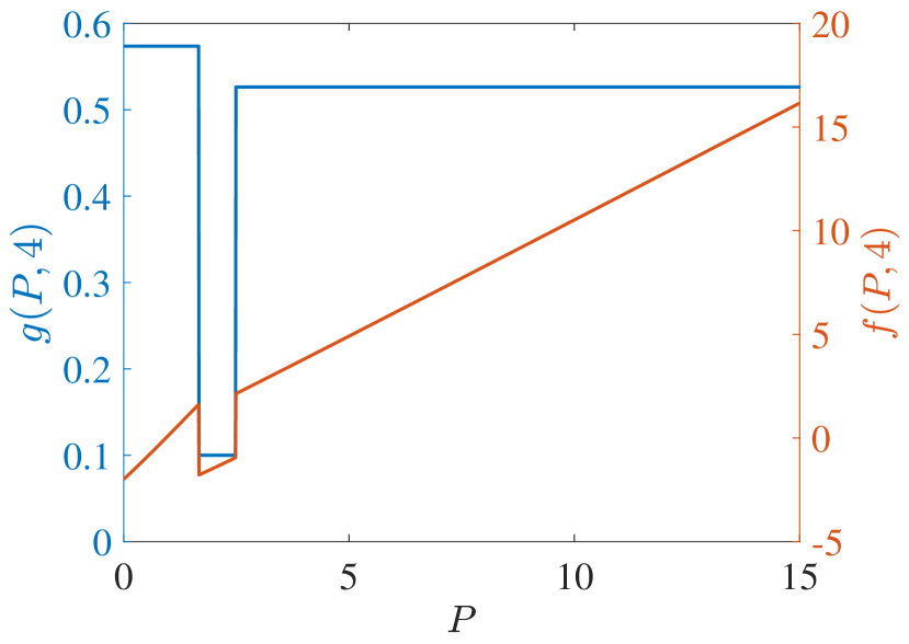
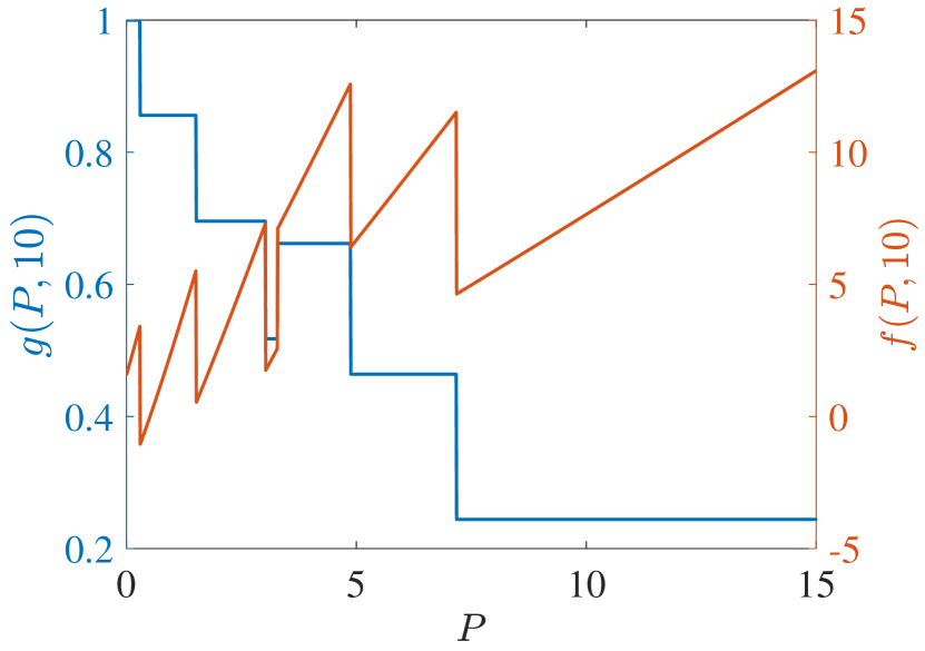
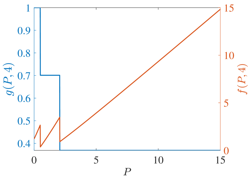
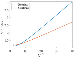
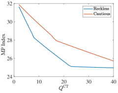
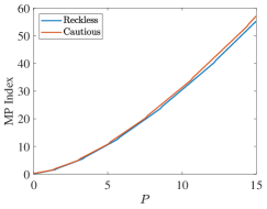
Regarding PCL-indexability condition (PCLI2), namely that the MP index defined by $\mathrm{mp}^{*}(P)\triangleq f(P,P)/g(P,P)$ be bounded below, continuous and monotone non-decreasing, Fig. 4 plots the MP index with choices of $Q^{\text{CT}}$ and $P$ for the two target types considered. Figs. 4 (c) and (d) show the MP index vs. $P$ for $Q^{\text{CT}}=4,10$, respectively. The plots are clearly consistent with condition (PCLI2), which has been observed in other instances not reported here.

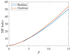
Fig. 4 (a) and (b) further show the MP index vs. $Q^{\text{CT}}\in[0,40]$ for states $P=1,10$, respectively. When the state $P$ is small, the long-term cost is predominantly influenced by $Q^{\text{CT}}$. Consequently, with the same $P=1$, the reckless target with a higher $Q^{\text{CT}}$ will obtain a higher MP index value. Otherwise, with a large $P=10$, prioritizing the long-term cost minimization, the MP index policy will sacrifice the immediate cost at the current time and track the target with higher $Q^{\text{CT}}$ after a certain number of time steps. That is, the target with a lower $Q^{\text{CT}}$ is tracked currently. Hence, the MP index will decrease over $Q^{\text{CT}}$. Due to the higher probability of a cautious target acquiring a lower cost with the same state $P$ and $Q^{\text{CT}}$ under action 1, cautious targets obtain a higher index than reckless targets in all states, which indicates that the MP index policy takes the tracking action prudently for reckless targets.

In summary, the above partial numerical evidence that the model of concern satisfies PCL-indexability conditions (PCLI1) and (PCLI2), and hence we shall further use the MP index as a surrogate of the Whittle index, and refer to it as the Whittle index.

In this subsection, $N=8$ smart targets are tracked by the radars network with $K=1,\ldots,3$ radars. For each target, the radar tracking time horizon $T=100$ s and $\beta=0.9$. We set up the Whittle index policy with the truncated time $\tau=100$, the TEV index policy where $\lambda^{\text{TEV}}(P)=d*P$ , and the myopic policy that degenerates to $\mathrm{mp}^{\text{myopic}}=d*(\phi^{0}(P,\bm{u}^{0})-\phi^{1}(P,\bm{u}^{1}))$ to assess tracking performances.

The parameters $F_{n}^{\text{CV}}$, $F_{n}^{\text{CT}}$, $Q_{n}^{\text{CV}}$, $h_{n}$ of target $n$ and $H$, $R$ are assumed the same as Section IV-A, $n=1,\ldots,N$. The initial state $P_{n,0}\sim\mathrm{U}(0,2)$. Then, we define three scenarios with only reckless type, cautious type, and each type of target accounting for 4, where the process noise variance $Q_{n}^{\text{CT}}=\{2,2,\ldots,2\}$ and $\{2,3,\ldots,9\}$ in the first two scenarios, respectively; Otherwise, $Q_{n}^{\text{CT}}=\{2,2,\ldots,2\}$ and $\{2,3,4,5,2,3,4,5\}$ in the third scenario. We assume $d_{n}=5$, $n=1$ and $d_{n}=1$, $n\neq 1$ in the first two scenarios. Moreover, $d_{n}=5$ for reckless targets and $d_{n}=1$ for cautious targets in the third scenario.

Table I, II, III show the discounted objective performance in three policies. Each policy is analyzed by varying the optional number $K$ of radars and $N_{mc}=100$ Monte Carlo simulations. When all the targets are homogeneous and heterogeneous, the Whittle index policy can obtain the best scheduling performance and outperform the TEV index and myopic policies. The myopic policy considers the one-step cost optimization, which is beneficial to the different types of targets; While the TEV index policy is not insensitive to the variation of targets. Consequently, the performance of the myopic policy is better than the TEV policy. Hence, the simulation results of all the scenarios show the superiority of the Whittle index policies.

Within this section, we validate the near optimality of the Whittle index policy discussed in Section III-C through different $d_{n}$ and $Q_{n}^{\text{CT}}$, when the number of radars and targets increases with a fixed ratio $\xi=K/N=1/4$. The parameters $F_{n}^{\text{CV}}$, $F_{n}^{\text{CT}}$, $Q_{n}^{\text{CV}}$, $h_{n}$ of target $n$ and $H$, $R$ are assumed the same as Section IV-B.

We first assume three scenarios, where $d_{n}=1$, $n=1,\ldots,N$. Three scenarios are divided by the types of targets, including all the reckless targets, all the cautious targets, and each type of target accounts for $50\%$. For each target $n$, let ${{P}}_{n,0}=0.01$. In addition, the process noise variances of the three scenarios are $Q_{n}^{\text{CT}}=\{2,\ldots,N+1\}$, $Q_{n}^{\text{CT}}=\{2,\ldots,N+1\}$, $Q_{n}^{\text{CT}}=\{2,\ldots,N/2+1,2,\ldots,N/2+1\}$, $n=1,\ldots,N$, respectively. We modify the simulation population by letting $K$ vary. For each scenario, the Whittle index truncates the corresponding infinite series to $\tau=100$ terms with $\beta=0.9$, and performances are evaluated by $N_{mc}=100$ Monte Carlo simulations.

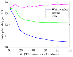
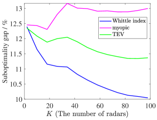
Through the calculations of the lower bound in Section III-B, we derive the simulation results about the suboptimality gap between the lower bound per target and the objective per target of index policies, as shown in Fig. 5, respectively.

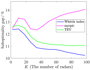
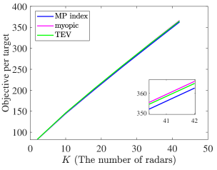
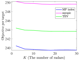
Different from the above three scenarios, we assume another scenario with the ratio $\xi=K/N=1/4$. Firstly, there are $50\%$ reckless targets with $d_{n}=5$ in the population of $N$ and others are cautious with $d_{n}=1$. Secondly, we assume that all of the targets share the identical process noise variance $Q_{n}^{\text{CT}}=4$. Other simulation parameters of each target are the same as the above three scenarios. The initial state for each target $n$ is assumed to be ${{P}}_{n,0}\sim\mathrm{U}(0,2)$. We modify the simulation population by letting $K$ vary. The results are shown in Fig. 6.

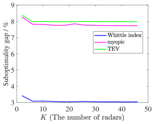
Fig. 5 shows that the suboptimality gaps of the Whittle index policy and the TEV index policy decrease as the radar system scale increases. However, the suboptimality gap of the Whittle index policy converges to a lower level, which is lower than $10.5\%$, while the TEV index policy obtains a larger suboptimality gap. Unfortunately, the myopic policy has the worst performance and the suboptimality gap may increase as $K$ grows. In Fig. 6, the Whittle index policy also achieves the lowest suboptimality gap, which is stable at about $3.0\%$. While the TEV index policy and the myopic policy obtain $8.0\%$ and $7.8\%$, respectively. Consequently, the Whittle index policy obtains lower objectives per target than other policies and the lowest suboptimality gap in all four scenarios.

Above all, the near optimality of the Whittle index policy is validated in this beam scheduling problem. When all the targets are homogeneous in different groups related to the target type and target parameters in Fig. 6, except ${{P}}_{n,0}\sim\mathrm{U}(0,2)$, and the suboptimality gap of the Whittle index policy is approximately stable at the lowest level. Accordingly, the Whittle index policy can efficiently solve the beam scheduling problem with real-valued TEV states and achieve better non-myopic performance than other greedy policies.

In this subsection, we attempt to expand the application of the MP index policy to the multi-dimensional states case. $N=8$ targets are tracked by the radar network with $K=1,\ldots,3$ radars. For each target, the radar tracking time horizon $T=100$ s. The MP index policy, the TEC index policy, and the myopic policy are described in Section III-G to assess the tracking performance.

Let $\bm{x}_{n,t}=\left[x_{n,t},\dot{x}_{n,t},y_{n,t},\dot{y}_{n,t}\right]^{\prime}$ be the dynamic state of target $n$ at time $t$, where $[x_{n,t},y_{n,t}]$ represents the position of target $n$ at time $t$, $[\dot{x}_{n,t},\dot{y}_{n,t}]$ is the velocity of target $n$ at time $t$. The state transition matrices corresponding to the CV and CT model are given by

where $T_{s}=1$ denotes the tracking time interval, $\omega$ denotes the turn rate, and $\otimes$ represents the Kronecker product.

The process noise variance matrix

References

- [1] A. M. Haimovich, R. S. Blum, and L. J. Cimini, “MIMO radar with widely separated antennas,” IEEE Signal Processing Magazine, vol. 25, no. 1, pp. 116–129, 2007.
- [2] W. Zhang, C. Shi, J. Zhou, and R. Lv, “Joint aperture and transmit resource allocation strategy for multi-target localization in phased array radar network,” IEEE Transactions on Aerospace and Electronic Systems, vol. 59, no. 2, pp. 1551–1565, 2023.
- [3] J. Yan, H. Jiao, W. Pu, C. Shi, J. Dai, and H. Liu, “Radar sensor network resource allocation for fused target tracking: a brief review,” Information Fusion, vol. 86, pp. 104–115, 2022.
- [4] C. Kreucher, D. Blatt, A. Hero, and K. Kastella, “Adaptive multi-modality sensor scheduling for detection and tracking of smart targets,” Digital Signal Processing, vol. 16, no. 5, pp. 546–567, 2006.
- [5] C. O. Savage and B. F. La Scala, “Sensor management for tracking smart targets,” Digital Signal Processing, vol. 19, no. 6, pp. 968–977, 2009.
- [6] Z. Zhang and G. Shan, “Non-myopic sensor scheduling to track multiple reactive targets,” IET Signal Processing, vol. 9, no. 1, pp. 37–47, 2015.
- [7] A. O. Hero, D. Castañón, D. Cochran, and K. Kastella, Foundations and applications of sensor management. Springer Science & Business Media, 2007.
- [8] M. R. Taner, O. E. Karasan, and E. Yavuzturk, “Scheduling beams with different priorities on a military surveillance radar,” IEEE Transactions on Aerospace and Electronic Systems, vol. 48, no. 2, pp. 1725–1739, 2012.
- [9] H. Godrich, A. P. Petropulu, and H. V. Poor, “Sensor selection in distributed multiple-radar architectures for localization: A knapsack problem formulation,” IEEE Transactions on Signal Processing, vol. 60, no. 1, pp. 247–260, 2011.
- [10] G. Zhang, J. Xie, H. Zhang, Z. Li, and C. Qi, “Dynamic antenna selection for colocated MIMO radar,” Remote Sensing, vol. 14, no. 12, p. 2912, 2022.
- [11] H. Zhang, J. Shi, Q. Zhang, B. Zong, and J. Xie, “Antenna selection for target tracking in collocated MIMO radar,” IEEE Transactions on Aerospace and Electronic Systems, vol. 57, no. 1, pp. 423–436, 2020.
- [12] J. Dai, J. Yan, W. Pu, H. Liu, and M. S. Greco, “Adaptive channel assignment for maneuvering target tracking in multistatic passive radar,” IEEE Transactions on Aerospace and Electronic Systems, vol. 59, no. 3, pp. 2780–2793, 2023.
- [13] W. Yi, Y. Yuan, R. Hoseinnezhad, and L. Kong, “Resource scheduling for distributed multi-target tracking in netted colocated MIMO radar systems,” IEEE Transactions on Signal Processing, vol. 68, pp. 1602–1617, 2020.
- [14] H. Zhang, W. Liu, J. Xie, Z. Zhang, and W. Lu, “Joint subarray selection and power allocation for cognitive target tracking in large-scale MIMO radar networks,” IEEE Systems Journal, vol. 14, no. 2, pp. 2569–2580, 2020.
- [15] M. Xie, W. Yi, T. Kirubarajan, and L. Kong, “Joint node selection and power allocation strategy for multitarget tracking in decentralized radar networks,” IEEE Transactions on Signal Processing, vol. 66, no. 3, pp. 729–743, 2017.
- [16] C. Shi, Y. Wang, S. Salous, J. Zhou, and J. Yan, “Joint transmit resource management and waveform selection strategy for target tracking in distributed phased array radar network,” IEEE Transactions on Aerospace and Electronic Systems, vol. 58, no. 4, pp. 2762–2778, 2021.
- [17] J. Yan, W. Pu, S. Zhou, H. Liu, and M. S. Greco, “Optimal resource allocation for asynchronous multiple targets tracking in heterogeneous radar networks,” IEEE Transactions on Signal Processing, vol. 68, pp. 4055–4068, 2020.
- [18] J. Yan, W. Pu, S. Zhou, H. Liu, and Z. Bao, “Collaborative detection and power allocation framework for target tracking in multiple radar system,” Information Fusion, vol. 55, pp. 173–183, 2020.
- [19] C. Pang and G. Shan, “Sensor scheduling based on risk for target tracking,” IEEE Sensors Journal, vol. 19, no. 18, pp. 8224–8232, 2019.
- [20] V. Krishnamurthy, Partially Observed Markov Decision Processes: From Filtering to Controlled Sensing. Cambridge, UK: Cambridge University Press, 2016.
- [21] C. Kreucher, A. O. Hero, K. Kastella, and D. Chang, “Efficient methods of non-myopic sensor management for multitarget tracking,” in 2004 43rd IEEE Conference on Decision and Control (CDC)(IEEE Cat. No. 04CH37601), vol. 1. IEEE, 2004, pp. 722–727.
- [22] C. M. Kreucher and A. O. Hero, “Monte Carlo methods for sensor management in target tracking,” in 2006 IEEE Nonlinear Statistical Signal Processing Workshop. IEEE, 2006, pp. 232–237.
- [23] X. Gongguo, S. Ganlin, and D. Xiusheng, “Non-myopic scheduling method of mobile sensors for manoeuvring target tracking,” IET Radar, Sonar & Navigation, vol. 13, no. 11, pp. 1899–1908, 2019.
- [24] G. Shan, G. Xu, and C. Qiao, “A non-myopic scheduling method of radar sensors for maneuvering target tracking and radiation control,” Defence Technology, vol. 16, no. 1, pp. 242–250, 2020.
- [25] Q. Dong and C. Pang, “Risk-based non-myopic sensor scheduling in target threat level assessment,” IEEE Access, vol. 9, pp. 76 379–76 394, 2021.
- [26] G. Shan and Z. Zhang, “Non-myopic sensor scheduling for low radiation risk tracking using mixed POMDP,” Transactions of the Institute of Measurement and Control, vol. 39, no. 2, pp. 230–243, 2017.
- [27] S. Howard, S. Suvorova, and B. Moran, “Optimal policy for scheduling of Gauss–Markov systems,” in Proceedings of the Seventh International Conference on Information Fusion. Citeseer, 2004, pp. 888–892.
- [28] P. Whittle, “Restless bandits: Activity allocation in a changing world,” Journal of Applied Probability, vol. 25, no. A, pp. 287–298, 1988.
- [29] J. C. Gittins, “Bandit processes and dynamic allocation indices,” Journal of the Royal Statistical Society: Series B (Methodological), vol. 41, no. 2, pp. 148–164, 1979.
- [30] V. Krishnamurthy and R. J. Evans, “Hidden Markov model multiarm bandits: A methodology for beam scheduling in multitarget tracking,” IEEE Transactions on Signal Processing, vol. 49, no. 12, pp. 2893–2908, 2001.
- [31] J. Gittins, K. Glazebrook, and R. Weber, Multi-armed bandit allocation indices. John Wiley & Sons, 2011.
- [32] C. H. Papadimitriou and J. N. Tsitsiklis, “The complexity of optimal queuing network control,” Mathematics of Operations Research, vol. 24, no. 2, pp. 293–305, 1999.
- [33] J. Niño-Mora, “Markovian restless bandits and index policies: A review,” Mathematics, vol. 11, no. 7, p. 1639, 2023.
- [34] R. R. Weber and G. Weiss, “On an index policy for restless bandits,” Journal of applied probability, vol. 27, no. 3, pp. 637–648, 1990.
- [35] B. F. La Scala and B. Moran, “Optimal target tracking with restless bandits,” Digital Signal Processing, vol. 16, no. 5, pp. 479–487, 2006.
- [36] C. R. Dance and T. Silander, “When are Kalman-filter restless bandits indexable?” in Proceedings of the 28th Conference on Neural Information Processing Systems (NIPS), Montreal, Canada. Cambridge, MA: MIT Press, 2015, pp. 1711–1719.
- [37] K. Liu and Q. Zhao, “Indexability of restless bandit problems and optimality of whittle index for dynamic multichannel access,” IEEE Transactions on Information Theory, vol. 56, no. 11, pp. 5547–5567, 2010.
- [38] J. Niño-Mora and S. S. Villar, “Sensor scheduling for hunting elusive hiding targets via Whittle’s restless bandit index policy,” in International Conference on NETwork Games, Control and Optimization (NetGCooP 2011). IEEE, 2011, pp. 1–8.
- [39] J. Wang, X. Ren, Y. Mo, and L. Shi, “Whittle index policy for dynamic multichannel allocation in remote state estimation,” IEEE Transactions on Automatic Control, vol. 65, no. 2, pp. 591–603, 2019.
- [40] J. Niño-Mora, “Restless bandits, partial conservation laws and indexability,” Advances in Applied Probability, vol. 33, no. 1, pp. 76–98, 2001.
- [41] ——, “Dynamic allocation indices for restless projects and queueing admission control: A polyhedral approach,” Mathematical programming, vol. 93, no. 3, pp. 361–413, 2002.
- [42] ——, “Restless bandit marginal productivity indices, diminishing returns and optimal control of make-to-order/make-to-stock M/G/1 queues,” Mathematics of Operations Research, vol. 31, no. 1, pp. 50–84, 2006.
- [43] ——, “A verification theorem for threshold-indexability of real-state discounted restless bandits,” Mathematics of Operations Research, vol. 45, no. 2, pp. 465–496, 2020.
- [44] ——, “Conservation laws and related applications,” in Wiley Encyclopedia of Operations Research and Management Science. New York, NY, USA: Wiley Online Library, 2011.
- [45] ——, “An index policy for dynamic fading-channel allocation to heterogeneous mobile users with partial observations,” in Proceedings of the 4th EuroNGI Conference on Next Generation Internet Networks (NGI), Krakow, Poland. New York, NY, USA: IEEE, 2008, pp. 231–238.
- [46] J. Niño-Mora and S. S. Villar, “Multitarget tracking via restless bandit marginal productivity indices and Kalman filter in discrete time,” in Proceedings of the Joint 48th IEEE Conference on Decision and Control (CDC) / 28th Chinese Control Conference (CCC), Shanghai, China. New York, NY, USA: IEEE, 2009, pp. 2905–2910.
- [47] J. Niño-Mora, “Whittle’s index policy for multi-target tracking with jamming and nondetections,” in Proceedings of the 23rd International Conference on Analytical and Stochastic Modelling Techniques and Applications (ASMTA), Cardiff, Wales. Cham, Switzerland: Springer, 2016, pp. 210–222.
- [48] ——, “A verification theorem for indexability of discrete time real state discounted restless bandits,” arXiv:1512.04403, 2015.
- [49] C. R. Dance and T. Silander, “Optimal policies for observing time series and related restless bandit problems,” The Journal of Machine Learning Research, vol. 20, no. 1, pp. 1218–1310, 2019.
- [50] F. Yang and X. Luo, “A restless MAB-based index policy for UL pilot allocation in massive MIMO over Gauss–Markov fading channels,” IEEE Transactions on Vehicular Technology, vol. 69, no. 3, pp. 3034–3047, 2020.
- [51] R. Visina, Y. Bar-Shalom, and P. Willett, “Multiple-model estimators for tracking sharply maneuvering ground targets,” IEEE Transactions on Aerospace and Electronic Systems, vol. 54, no. 3, pp. 1404–1414, 2018.
- [52] W. D. Blair and Y. Bar-Shalom, “MSE design of nearly constant velocity Kalman filters for tracking targets with deterministic maneuvers,” IEEE Transactions on Aerospace and Electronic Systems, vol. 59, no. 4, pp. 4180–4191, 2023.
- [53] D. B. Brown and J. E. Smith, “Index policies and performance bounds for dynamic selection problems,” Management Science, vol. 66, no. 7, pp. 3029–3050, 2020.