Non-Markovian Reduced Models to Unravel Transitions in Non-equilibrium Systems
Abstract
This work proposes a general framework for analyzing noise-driven transitions in spatially extended non-equilibrium systems and explains the emergence of coherent patterns beyond the instability onset. The framework relies on stochastic parameterization formulas to reduce the complexity of the original equations while preserving the essential dynamical effects of unresolved scales. The approach is flexible and operates for both Gaussian noise and non-Gaussian noise with jumps.
Our stochastic parameterization formulas offer two key advantages. First, they can approximate stochastic invariant manifolds when these manifolds exist. Second, even when such manifolds break down, our formulas can be adapted through a simple optimization of its constitutive parameters. This allows us to handle scenarios with weak time-scale separation where the system has undergone multiple transitions, resulting in large-amplitude solutions not captured by invariant manifolds or other time-scale separation methods.
The optimized stochastic parameterizations capture then how small-scale noise impacts larger scales through the system’s nonlinear interactions. This effect is achieved by the very fabric of our parameterizations incorporating non-Markovian (memory-dependent) coefficients into the reduced equation. These coefficients account for the noise’s past influence, not just its current value, using a finite memory length that is selected for optimal performance. The specific “memory” function, which determines how this past influence is weighted, depends on both the strength of the noise and how it interacts with the system’s nonlinearities.
Remarkably, training our theory-guided reduced models on a single noise path effectively learns the optimal memory length for out-of-sample predictions. This approach retains indeed good accuracy in predicting noise-induced transitions, including rare events, when tested against a large ensemble of different noise paths. This success stems from our “hybrid” approach, which combines analytical understanding with data-driven learning. This combination avoids a key limitation of purely data-driven methods: their struggle to generalize to unseen scenarios, also known as the “extrapolation problem.”
pacs:
05.45.-a, 89.75.-kI Introduction
Non-equilibrium systems are irreversible systems characterized by a continuous flow of energy that is driven by external forces or internal fluctuations. There are many different types of non-equilibrium systems, and they can be found in a wide variety of fields, including physics, chemistry, biology, and engineering. Non-equilibrium systems can exhibit complex behavior, including self-organization, pattern formation, and chaos. These complex behaviors arise from the interplay of nonlinear dynamics and statistical fluctuations. The emergence of coherent, complex patterns is ubiquitous in many spatially extended non-equilibrium systems; see e.g. [1, 2, 3, 4, 5, 6, 7, 8, 9, 10]. Mechanisms to explain the emergence of these patterns include the development of instability saturated by nonlinear effects whose calculations can be conducted typically near the onset of linear instability; see e.g. [11, 12]. Historically, hydrodynamic systems have been commonly used as prototypes to study instabilities out of equilibrium in spatially extended systems, from both an experimental and a theoretical point of view [13, 3].
To describe how physical instability develops in such systems with infinitely many degrees of freedom, we often focus on the amplitudes’ temporal evolution of specific normal modes. The latter correspond typically to those that are mildly unstable and that are only slightly damped in linear theory. When the number of these nearly marginal modes is finite, their amplitudes are governed by ordinary differential equations (ODEs) in which the growth rates of the linear theory have been renormalized by nonlinear terms [1, 11, 3, 12]. Intuitively, the reason for this reduction is a simple separation of time scales. Modes that have just crossed the imaginary axis have a small real part and are evolving slowly on long time scales, all the other fast modes rapidly adapting themselves to these slow modes.
However, for non-equilibrium systems away from the onset of linear instability, such as when the Reynolds number for a fluid flow increases far beyond a laminar regime, the emergence of coherent patterns does not fit within this instability/nonlinear saturation theory as the reduction principle of the fast modes onto the slow ones breaks down [11] and calls for new reduction techniques to explain emergence. Furthermore, in the presence of random fluctuations, reduced equations under the form of deterministic ODEs are inherently incapable to capture phenomena like noise-induced transitions. Noise can have unexpected outcomes such as altering the sequence of transitions, possibly suppressing instabilities [14], the onset of turbulence [15] or, to the opposite, exciting transitions [16, 7]. Examples in which noise-induced transitions have an important role include the generation of convective rolls [17, 18], electroconvection in nematic liquid crystals [16, 19], certain oceanic flows [20, 21], and climate phenomena [22, 23, 24, 25].
This work aims to gain deeper insights into the efficient derivation of reduced models for such non-equilibrium systems subject to random fluctuations [3, 7]. In that respect, we seek reduced models able to capture the emergence of noise-driven spatiotemporal patterns and predict their transitions triggered by the subtle coupling between noise and the nonlinear dynamics. Our overall goal is to develop a unified framework for identifying the key variables and their interactions (parameterization) in complex systems undergoing noise-driven transitions. We specifically focus on systems that have experienced multiple branching points (bifurcations), leading to high-multiplicity regimes with numerous co-existing metastable states whose amplitude is relatively large (order one or more) resulting from a combination of strong noise, inherent nonlinear dynamics, or both. The purpose is thus to address limitations of existing approaches like amplitude equations and center manifold techniques in dealing with such regimes.
To address these limitations, the framework of optimal parameterizing manifolds (OPMs) introduced in [26, 27, 28] for forced-dissipative systems offers a powerful solution. This framework allows for the efficient derivation of parameterizations away from the onset of instability, achieved through continuous deformations of near-onset parameterizations that are optimized by data-driven minimization. Typically, the loss function involves a natural discrepancy metric measuring the defect of parameterization of the unresolved variables by the resolved ones. The parameterizations that are optimized are derived from the governing equations by means of backward-forward systems providing useful approximations of the unstable growth saturated by the nonlinear terms, even when the spectral gap between the stable and unstable modes is small [27, 29, 28]. These approximations, once optimized, do not suffer indeed the restrictions of invariant manifolds (spectral gap condition [27, Eq. (2.18)]) allowing to handle situations with e.g. weak time-scale separation between the resolved and unresolved modes.
In this article, we carry over this variational approach to the case of spatially extended non-equilibrium systems within the framework of stochastic partial differential equations (SPDEs). In particular, we extend the parameterization formulas obtained in [30, 29, 31] for SPDEs driven by multiplicative noise (parameter noise [18, 7]), to SPDEs driven, beyond this onset, by more realistic, spatio-temporal noise either of Gaussian or of non-Gaussian nature with jumps. For this class of SPDEs, our framework allows for dealing with the important case of cutoff scales larger than the scales forced stochastically.
For this forcing scenario, the stochastic parameterizations derived in this work, give rise to reduced systems taking the form of stochastic differential equations (SDEs) with non-Markovian, path-dependent coefficients depending on the noise’s past; see e.g. Section V.2 below. We mention that many time series records from real-world datasets, are known to exhibit long-term memory. This is the case of long-range memory features assumed to represent the internal variability of the climate on time scales from years to centuries [32, 33, 34, 35]. There, the surface temperature is considered as a superposition of internal variability (the response to stochastic forcing) and a forced signal which is the linear response to external forcing. The background variability may be modeled using a stochastic process with memory, or a different process that incorporates non-Gaussianity if this is considered more appropriate [36]. As will become apparent at the end of this paper, our reduction approach is adaptable to PDEs under the influence of stochastic forcing with long-range dependence; see Section IX.
In parallel and since Hasselmann’s seminal work [37], several climate models have been incorporating stochastic forcing to represent unresolved processes [38, 39, 40, 41, 42, 43]. Our approach shows that reduced models derived from these complex systems are expected to exhibit finite-range memory effects depending on the past history of the stochastic forcing, even if the latter is white in time. These exogenous memory effects, stemming from the forcing noise’s history, are distinct from endogenous memory effects encountered in the reduction of nonlinear, unforced systems [44, 45, 43]. The latter, predicted by the Mori-Zwanzig (MZ) theory, are functionals of the past of the resolved state variables. Endogenous memory effects often appear when the validity of the conditional expectation in the MZ expansion, breaks down [46, 26, 47, 43]. The exogenous memory effects dealt with in this work, have a different origin, arising as soon as the cutoff scale is larger than the scales forced stochastically.
It is worth mentioning that reduced models with non-Markovian coefficients responsible for such exogenous memory effects, have been encountered in the reduction of stochastic systems driven by white noise, albeit near a change of stability. These are obtained from reduction approaches benefiting from timescale separation such as stochastic normal forms [48, 49, 50], stochastic invariant manifold approximations [51, 30, 29, 31], or multiscale methods [52, 53, 54, 55]. Our reduction approach is not limited to timescale separation.
In that respect, our reduction framework is tested against a stochastic Allen-Cahn equation (sACE), a powerful tool for modeling non-equilibrium phase transitions in various scientific fields [1, 3, 56, 57]. The latter model is set in a parameter regime with weak timescale separation and far from the instability onset, in which the system exhibits multiple coexisting metastable states connected to the basic state through rare or typical stochastic transition paths.
We show that our resulting OPM reduced systems, when trained over a single path, are not only able to retain a remarkable predictive power to emulate ensemble statistics (correlations, power spectra, etc.) obtained as average over a large ensemble of noise realizations, but also anticipate what are the system’s typical and rare metastable states and their statistics of occurrence. The OPM reduced system’s ability to reproduce accurately such transitions is rooted in its very structure. Its coefficients are nonlinear functionals of the aforementioned non-Markovian terms (see Eq. (85) below) allowing for an accurate representation of the genuine nonlinear interactions between noise and nonlinear terms in the original sACE, which drive fluctuations in the large-mode amplitudes.
We emphasize, that because the cutoff scale, defining the retained large-scale dynamics, is chosen here to be larger than the forcing scale, any deterministic reduction (e.g. Galerkin, invariant manifold, etc.) would filter out the underlying noise’s effects. This leaves them blind to the subtle fluctuations driving the system’s behavior and leading eventually to stochastic transitions. In contrast, our stochastic parameterization approach sees right through this filter. It tracks how the noise, acting in the “unseen” part of the system, interacts with the resolved modes through our reduction method’s non-Markovian coefficients.
To demonstrate the broad applicability of our reduction approach, we apply it in Section VI to another significant class of spatially extended non-equilibrium systems: jump-driven SPDEs. The unforced, nonlinear dynamics is here chosen to exhibit an S-shaped solution curve. Many systems sharing this attribute are indicative of multistability, tipping points, and hysteresis. Such behaviors are observed in various fields, including combustion theory [58, 59], plasma physics [60, 61], ecology [9], neuroscience [62], climate science [63, 64], and oceanography [65, 66]. By understanding the complex interactions between noise and nonlinearity into these phenomena, we can gain insights into critical transitions and tipping points, which are increasingly relevant to addressing global challenges like climate change [67, 68, 69, 70, 43].
Jump processes offer a powerful tool for modeling complex systems with non-smooth dynamics. They offer valuable insights into multistable behaviors [71, 72] and have been applied to various real-world phenomena, such as paleoclimate events [73, 36], chaotic transport [74], atmospheric dynamics [75, 76, 77, 78, 79, 80], and cloud physics [81, 82].
SPDEs driven by jump processes are gaining increasing attention in applications [83]. For instance, jump processes can replace (non-smooth) ”if-then” conditions in such models, enabling more efficient simulations [80]. Nevertheless, efficient reduction techniques to disentangle the jump interactions with other smoother nonlinear components of the model, are still under development [84, 85, 86]. Our stochastic parameterization framework provides a promising solution in this direction, as demonstrated in Section VI. By capturing the intricate interplay between jump noise and nonlinear dynamics within the reduced equations, our approach can significantly simplify the analysis of such complex systems.
II Invariance Equation and Approximations
II.1 Spatially extended non-equilibrium systems
This article is concerned with the efficient reduction of spatially extended non-equilibrium systems. To do so, we work within the framework of Stochastic Equations in Infinite Dimensions [87] and its Ergodic Theory [88]. Formally, these equations take the following form
| (1) |
in which is a stochastic process, either composed of Brownian motions or jump processes and whose exact structure is specified below. This formalism provides a convenient way to analyze stochastic partial differential equations (SPDEs) by means of semigroup theory [89, 90], in which the unknown evolves typically in a Hilbert space .
The operator represents a linear differential operator while is a nonlinear operator that accounts for the nonlinear terms. Both of these operators may involve loss of spatial regularity when applied to a function in . To have a consistent existence theory of solutions and their stochastic invariant manifolds for SPDEs requires to take into account such loss of regularity effects [87, 88].
General assumptions encountered in applications are made on the linear operator following [89]. More specifically, we assume
| (2) |
where is sectorial with domain which is compactly and densely embedded in . We assume also that is stable, while is a low-order perturbation of , i.e. is a bounded linear operator such that for some in . We refer to [89, Sec. 1.4] for an intuitive presentation of fractional power of an operator and characterization of the so-called operator domain . In practice, the choice of should match the loss of regularity effects caused by the nonlinear terms so that
is a well-defined -smooth mapping that satisfies , (tangency condition), and
| (3) |
with , and denoting the leading-order operator (on ) in the Taylor expansion of , near the origin. A broad class of spatially extended stochastic equations from physics can be recasted into this framework (see [91, 87, 30, 92, 31] for examples), as well as time-delay systems subject to stochastic disturbances [82, 93].
Throughout this article, we assume that the driving noise in Eq. (1) is an -valued stochastic process that takes the form
| (4) |
where the are eigenmodes of , the denote either a finite family of mutually independent jump processes, or mutually independent Brownian motions, , over their relevant probability space endowed with its canonical probability measure and filtration ; see e.g. [50, Appendix A.3].
Within this framework, the reduction of spatially extended non-equilibrium systems is organized in terms of resolved and unresolved spatial scales. The resolved scales are typically spanned by large wavenumbers and the unresolved by smaller ones. In that respect, the eigenmodes of the operator plays a central role throughout this paper to rank the spatial scales. Typically, we assume that the state space of resolved variables is spanned by the following modes
| (5) |
where the correspond to large-scale modes up to a cutoff-scale associated with some index (see Remark II.1). The subspace of unresolved modes is then the orthogonal complement of in , namely
| (6) |
To these subspaces, we associate their respective canonical projectors denoted by
| (7) |
Throughout Section III below and the remaining of this Section, we focus on the case of driving Brownian motions; the case of driving jump processes is dealt with in Section VI.
Our goal is to provide a general approach to derive reduced models that preserve the essential features of the large-scale dynamics without resolving the small scales.
We present hereafter and in Section III below, the formulas of the underlying small-scale parameterizations in the Gaussian noise case. The formalism is flexible and easily adaptable to the case of non-Gaussian noises with jumps such as discussed in Sections VI and VII, below.
Remark II.1
Within our working assumptions, the spectrum consists only of isolated eigenvalues with finite multiplicities. This combined with the sectorial property of implies that there are at most finitely many eigenvalues with a given real part. The sectorial property of also implies that the real part of the spectrum, , is bounded above (see also [94, Thm. II.4.18]). These two properties of allow us in turn to label elements in according to the lexicographical order which we adopt throughout this article:
| (8) |
such that for any we have either
| (9) |
or
| (10) |
This way, we can rely on a simple labeling of the eigenvalues/eigenmodes by positive integers to organize the resolved and unresolved scales and the corresponding parameterization formulas derived hereafter. In practice, when the spatial domain is 2D or 3D, it is usually physically more intuitive to label the eigenelements by wave vectors. The parameterization formulas presented below can be easily recast within this convention; see e.g. [95].
II.2 Invariance equation and backward-forward systems
As mentioned in Introduction, this work extends the parameterization formulas in [27, 28] (designed for constant or time-dependent forcing) to the stochastic setting. In both deterministic and stochastic contexts, deriving the relevant parameterizations and reduced systems relies on solving Backward-Forward (BF) systems arising in the theory of invariant manifolds. Similar to [27, 28], our BF framework allows us to overcome limitations of traditional invariant manifolds, particularly the spectral gap condition ([27, Eq. (2.18)]). This restrictive condition, which requires large gaps in the spectrum of the operator , is bypassed through data-driven optimization (detailed in Section III.3) of the backward integration time over which the BF systems are integrated.
Before diving into the parameterization formulas retained to address these limitations (Section II.3), we recall the basics of reducing an SPDE to a Stochastic Invariant Manifold (SIM). In particular, this detour enables us to better appreciate the emergence of BF systems as a natural framework for parameterizations. For that purpose, adapting the approach from [30], we transform the SPDE reduction problem into the more tractable problem of reducing a PDE with random coefficients. This simplification makes the problem significantly more amenable to analysis than its original SPDE form.
To do so, consider the stationary solution to the Langevin equation
| (11) |
(Ornstein-Uhlenbeck (OU) process), where is defined in Eq. (4) with the corresponding mutually independent Brownian motions, , in place of the , i.e.:
| (12) |
Then, for each noise’s path , the change of variable
| (13) |
transforms the SPDE,
into the following PDE with random coefficients in the -variable:
| (14) |
Under standard conditions involving the spectral gap between the resolved and unresolved modes [96], the path-dependent PDE (14) admits a SIM, and the underlying stochastic SIM mapping, (), satisfies the stochastic invariance equation:
| (15) |
where denotes the operator acting on differentiable mappings from into , as follows:
| (16) |
with and .
To simplify, assume that and are chosen such that . Then in particular . Consider now the Lyapunov-Perron integral
| (17) |
where . In what follows, we denote by the Hermitian inner product on defined as , while denotes the leading-order term of order in the Taylor expansion of around , and denotes the -th eigenmode of the adjoint operator of adopting the same labelling convention as for ; see Remark. II.1. To the order we associate the set of indices , and denote by any subset of indices made of (possibly empty) of disjoint elements of .
We have then the following result.
Theorem II.1
Under the previous assumptions, assume furthermore that the following non-resonance condition holds, for any in , , and any subset such as defined above:
| (18) | ||||
with .
Then, the Lyapunov-Perron integral (Eq. (17)) is well-defined almost surely, and is a solution to the following homological equation with random coefficients:
| (19) |
Moreover, we observe that the integral is (formally) obtained as the limit, when goes to infinity, of the -solution to the following backward-forward (BF) auxiliary system:
| (20a) | |||
| (20b) | |||
| (20c) | |||
That is
| (21) |
where denotes the solution to Eq. (20b) at time , when initialized with at .
For a proof of this Theorem, see Appendix A. This theorem extends to the stochastic context Theorem III.1 of [28]. To simplify the notations, we omit below the -dependence in certain notations unless specified otherwise.
Theorem II.1 teaches us that solving the BF system (20) gives the solution to the homological equation (17) which is an approximation of the full invariance equation Eq. (15). In the deterministic setting, solutions to the homological equation (17) are known to provide actual approximations of the invariant manifolds with rigorous estimates; see [27, Theorem 1] and [28, Theorem III.1]. Such results extend to the case of SPDEs driven by multiplicative (parameter) noise; see [31, Theorem 2.1] and [30, Theorem 6.1 and Corollary 7.1]. It is not the scope of this article to deal with rigorous error estimates regarding the approximation problem of stochastic invariant manifolds for SPDEs driven by additive noise, but the rationale stays the same: solutions to the homological equation (17) or equivalently to the BF system (20) provide actual approximations of the underlying stochastic invariant manifolds, in the additive noise case as well.
Going back to the SPDE variable , the BF system (20) becomes
| (22a) | |||
| (22b) | |||
| (22c) | |||
Note that in Eq. (22), only the low-mode variable is forced stochastically, and thus from what precedes, , provides a legitimate approximation of the SIM at time when in the original SPDE, only the low modes are forced stochastically, i.e. in (12). In the next section, we consider the general case when the low and high modes are stochastically forced.
II.3 Approximations of fully coupled backward-forward systems
Backward-forward systems have been actually proposed in the literature for the construction of SIMs [97], through a different route than what presented above, i.e. without exploiting the invariance equation. The idea pursued in [97] is to envision SIMs as a fixed point of an integral form of the following fully coupled BF system
| (23a) | |||
| (23b) | |||
| (23c) | |||
where . Note that in Eq. (23), we do not assume here the noise term to be a finite sum of independent Brownian motions. In the case of an infinite sum one can thus covers the case of space-time white noise due to [98].
In any case, it is known that this type of fully coupled nonlinear problems involving backward stochastic equations does not have always solutions in general and we refer to [97, Proposition 3.1] for conditions on and ensuring existence of solutions and thus SIM. This (nonlinear) BF approach to SIM is also subject to a spectral gap condition that requires gap to be large enough as in [96].
Denoting by the solution to Eq. (23b) at , Proposition 3.4 of [97] ensures then that exists in and that this limit gives the sought SIM, i.e.
| (24) |
The SIM is thus obtained, almost surely, as the asymptotic graph of the mapping , when is sent to infinite.
Instead of relying on an integral form of Eq. (23), one can address though the existence and construction of a SIM via a more direct approach, exploiting iteration schemes built directly from Eq. (23). It is not the purpose of this article to analyze the convergence of such iterative schemes (subject also to a spectral gap condition as in [97]) but rather to illustrate how informative such schemes can be in designing stochastic parameterizations in practice.
To solve (23), given an initial guess, , we propose the following iterative scheme:
| (25a) | |||
| (25b) | |||
where and with in and . Here again, the first equation (Eq. (25a)) is integrated backward over , followed by a forward integration of the second equation (Eq. (25b)) over the same interval. To simplify the notations, we will often omit to point out the interval in the BF systems below.
To help interpret the parameterization produced by such an iterative scheme, we restrict momentarily ourselves to the case of a nonlinearity that is quadratic (denoted by ) and to noise terms that are scaled by a parameter . This case covers the important case of the Kardar–Parisi–Zhang equation [99]. The inclusion of this scaling factor allows us to group the terms constituting the stochastic parameterization according to powers of providing in particular useful small-noise expansions; see Eq. (30) below.
Under this working framework, if we start with , we get then
| (26) | ||||
which leads to
and
| (27) | ||||
To further make explicit that provides the stochastic parameterization we are seeking (after 2 iterations), we introduce
| (28) | ||||
We can then rewrite given in (LABEL:Eq_1st_iteration) as follows:
| (29) | ||||
By introducing additionally
we get for any the following explicit expressions
and
Let us denote by the projector onto the mode . Using the above identities in (LABEL:Eq_2nd_iteration), and setting , we get for ,
| (30) | ||||
where
| (31) | ||||
| (32) | ||||
and
with .
In the classical approximation theory of SIM, one is interested in conditions ensuring convergence of the integrals involved in the random coefficients and as , since (and its higher-order analogues with ) aims to approximate the SIM defined in Eq. (24). In our approach to stochastic parameterization, we do not restrict ourselves to such a limiting case but rather seek optimal backward integration time that minimizes a parameterization defect as explained below in Section III.3.
However, computing this parameterization defect involves the computation of the random coefficients in the course of time (see Eq. (53) below). The challenge is that the structure of and involves repeated stochastic convolutions in time, and as such one wants to avoid a direct computation by quadrature. We propose below an alternative and efficient way to compute such random coefficients, for a simpler, more brutal approximation than . As shown in Sections V and VI, this other class of stochastic parameterizations turns out to be highly performant for the important case where the stochastically forced scales are exclusively part of the neglected scales.
This approximation consists of setting in Eq. (LABEL:Eq_2nd_iteration), namely to deal with the stochastic parameterization
| (33) | ||||
after restoring as a more general nonlinearity than .
Note also that this parameterization is exactly the solution at of the following BF system
| (34a) | |||
| (34b) | |||
| (34c) | |||
with .
Section III.2 details an efficient computation of the single stochastic convolution in equation (33) using auxiliary ODEs with random coefficients. It is worth noting that previous SPDE reduction approaches have, in certain circumstances or under specific assumptions (e.g., as seen in [54, Eq. (2.2)] and [40, Eq. (2.10)]), deliberately opted to avoid directly computing these convolutions via quadrature [100, 101, 102].
The stochastic convolution in Eq. (33) accounts for finite-range memory effects stemming from the stochastic forcing to the original equation. Such terms have been encountered in the approximation of low-mode amplitudes, albeit in their asymptotic format when see e.g. [54, 103]. As shown in our examples below (Sections V and VI), stochastic convolution terms become crucial for efficient reduction when the cutoff scale, defining the retained large-scale dynamics, is larger than the forcing scale. There, we show furthermore that the finite-range memory content (measured by ) is a key factor for a skillful reduction when optimized properly. Also, as exemplified in applications, optimizing the nonlinear terms in Eq. (33) may turn to be of utmost importance to reproduce accurately the average motion of the SPDE dynamics; see Section V.5 below.
The efficient computation of repeated convolutions involved in the coefficients and is however more challenging and will be communicated elsewhere. This is not only a technical aspect though, as these repeated convolutions in given by Eq. (31) characterize important triad interactions reflecting how the noise interacts through the nonlinear terms into three groups: the low-low interactions in (), the low-high interactions in () and high-high interactions in (). By using the simpler parameterization defined in Eq. (33) we do not keep these interactions at the parameterization level, however as approximates the high-mode amplitude it still allows us to account for triad interactions into the corresponding reduced models; see e.g. Eq. (85) below.
III Non-Markovian Parameterizations: Formulas and Optimization
The previous discussion leads us to consider, for each , the following scale-aware BF systems
| (35a) | |||
| (35b) | |||
| (35c) | |||
where denotes the projector onto the mode . Here, is a free parameter to be adjusted, no longer condemned to approach as in the approximation theory of SIM discussed above. Note that compared to Eq. (34), we break down the forcing mode by mode for each high mode to allow for adjusting the free backward parameter, , per scale to parameterize (scale-awareness). This strategy allows for a greater degree of freedom to calibrate useful parameterizations, as will be apparent in applications dealt with in Sections V and VI.
Also, compared to Eq. (34), the initial condition for the forward integration in Eq. (35) is a scale-aware parameter in Eq. (35c). It is aimed at resolving the time-mean of the -th high-mode amplitude, with solving Eq. (1). In many applications, it is enough to set though.
In the following, we make explicit the stochastic parameterization obtained by integration of the BF system (35) for SPDEs with cubic nonlinear terms, for which the stochastically forced scales are part of the neglected scales.
III.1 Stochastic parameterizations for systems with cubic interactions
We consider
| (36) |
Here, is a partial differential operator as defined in (2) for a suitable ambient Hilbert space ; see also [29, Chap. 2]. The operators and are quadratic and cubic, respectively. Here again, we assume the eigenmodes of and its adjoint to form a bi-orthonormal basis of ; namely, the set of eigenmodes of and of each forms a Hilbert basis of , and they satisfy the bi-orthogonality condition , where denotes the Kronecker delta function. The noise term takes the form defined in Eq. (12). Stochastic equations such as Eq. (36) arise in many areas of physics such as in the description of phase separation [104, 105, 56], pattern formations [3, 7] or transitions in geophysical fluid models [20, 106, 107, 108, 25, 21, 31].
We assume that Eq. (36) is well-posed in the sense of possessing for any in a unique mild solution, i.e. there exists a stopping time such that the integral equation,
| (37) | ||||
possesses, almost surely, a unique solution in (continuous path in ) for all stopping time .
Here the stochastic integral can be represented as a series of one-dimensional Itô integrals
| (38) |
where the are the independent Brownian motions in (12). It is known that Eq. (36) admits a unique mild solution in with the right conditions on the coefficients of and (confining potential) [87]; see also [109, Prop. 3.4]. We refer to [88, 87] for background on the stochastic convolution term .
Throughout this section we assume that only a subset of unresolved modes in the decomposition (6) of are stochastically forced according to Eq. (12), namely that the following condition holds:
-
(H)
for in (12), and that there exists at least one index in such that .
In this case, the BF system (35) becomes
| (39) | ||||
The solution to Eq. (LABEL:Eq_BF_SPDEcubic) at provides a parameterization aimed at approximating the th high-mode amplitude, , of the SPDE solution when is equal to the low-mode amplitude . The BF system (LABEL:Eq_BF_SPDEcubic) can be solved analytically. Its solution provides the stochastic parameterization, , expressed, for , as the following stochastic nonlinear mapping of in :
| (40) | ||||
with
The stochastic term is given by
| (41) |
and as such, is dependent on the noise’s path and the “past” of the Wiener process forcing the -th scale: it conveys exogenous memory effects, i.e. it is non-Markovian in the sense of [110].
The coefficients and in (40) are given respectively by
| (42) |
while the coefficients and are given by
| (43) |
and
| (44) |
with and . From Eqns. (43) and (44), one observes that the parameter (depending on ) allows, in principle, for balancing the small denominators due to small spectral gaps, i.e. when the or the are small. This attribute is shared with the parameterization formulas obtained by the BF approach in the deterministic context; see [28, Remark III.1]. It plays an important role in the ability of our parameterizations to handle physically relevant situations with a weak time-scale separation; see Section V.5 below.
Remark III.1
In connection with the stochastic convolution in Eq. (33), we note that the stochastic terms in Eq. (40), involving the processes , , and , can be rewritten as a scalar stochastic integral, more precisely:
| (45) |
Note that the RHS in Eq. (45) is simply the projection of onto mode (Eq. (38)).
Equation (45) is a direct consequence of Itô’s formula applied to the product followed by integration over . Indeed, we have (dropping the -dependence),
by treating as zero due to Itô calculus [111].
By introducing now and denoting by the stochastic convolution , we arrive due to Eq. (41) at
| (46) |
which gives the relation , where we have set to simplify.
In the expression of given by Eq. (40), we opt for the expression involving the Riemann–Stieltjes integral for practical purpose. The latter can be indeed readily generalized to the case of jump noise (Eqns. (99)–(100) below) without relying on stochastic calculus involving a jump measure (Section VII).
In what follows we drop the dependence of on and sometimes on , unless specified. The parameterization of the neglected scales writes then as
| (47) |
with , and defined in Eq. (40).
We observe that letting approach infinity in Eq. (47) recovers Eq. (33) when . This implies that the manifold constructed from Eq. (47) can be viewed as a homotopic deformation of the SIM approximation defined in Eq. (33), controlled by the parameters .
This connection motivates utilizing the variational framework presented in [27, 28] to identify the “optimal” stochastic manifold within the family defined by Eq. (47). In Section III.3, we demonstrate that a simple data-driven minimization of a least-squares parameterization error, applied to a single training path, yields trained parameterizations (in terms of ) with remarkable predictive power. For instance, these parameterizations can be used to infer ensemble statistics of SPDEs for a large set of unseen paths during training.
However, unlike the deterministic case, the stochastic framework necessitates addressing the efficient simulation of the coefficients involved in Eq. (47) for optimization purposes. This challenge is tackled in the following subsection.
III.2 Non-Markovian path-dependent coefficients: Efficient simulation
Our stochastic parameterization given by (47) contains random coefficients , each of them involving an integral of the history of the Brownian motion making them non-Markovian in the sense of [110], i.e. depending on the noise path history. We present below an efficient mean to compute these random coefficients by solving auxiliary ODEs with path-dependent coefficients, avoiding this way the cumbersome computation of integrals over noise paths that would need to be updated at each time . This approach is used for the following purpose:
-
(i)
To find the optimal vector made of optimal backward-forward integration times and form in turn the stochastic optimal parameterization , and
-
(ii)
To efficiently simulate the corresponding optimal reduced system built from along with its path-dependent coefficients.
According to (41), the computation of boils down to the computation of the random integral
which is of the following form:
| (48) |
where , and due to assumption (H). We only need to consider the case that , since we consider here only cases in which the unstable modes are included within the space of resolved scales.
By taking time derivative on both sides of (48), we obtain that satisfies the following ODE with path-dependent coefficients also called a random differential equation (RDE):
| (49) |
Since , the linear part in (49) brings a stable contribution to (49). As a result, can be computed by integrating (49) forward in time starting at with initial datum given by:
| (50) |
where is computed using (48).
Now, to determine in (41) it is sufficient to observe that
| (51) |
The random coefficient is thus computed by using (51) after is computed by solving, forward in time, the corresponding RDE of the form (49) with initial datum
| (52) |
This way, we compute only the integral (52) and then propagate it through Eq. (49) to evaluate , instead of computing for each the integral in the definition (41). The resulting procedure is thus much more efficient to handle numerically than a direct computation of based on the integral formulation (41) which would involve a careful and computationally more expensive quadrature at each time-step. Note that a similar treatment has been adopted in [29, Chap. 5.3] for the computation of the time-dependent coefficients arising in stochastic parameterizations of SPDEs driven by linear multiplicative noise, and in [28, Sec. III.C.2] for the case of non-autonomous forcing.
III.3 Data-informed optimization and training path
Thanks to Section III.2, we are now in position to propose an efficient variational approach to optimize the stochastic parameterizations of Section III.1 in view of handling parameter regimes located away from the instability onset and thus a greater wealth of possible stochastic transitions.
Given a solution path to Eq. (36) available over an interval of length , we aim for determining the optimal parameterization (given by (40)) that minimizes—in the -variable—the following parameterization defect
| (53) |
for each . Here denotes the time-mean over while and denote the projections of onto the high-mode and the reduced state space , respectively. Figure 1 provides a schematic of the stochastic optimal parameterizing manifold (OPM) found this way.
The objective is obviously not to optimize the parameterizations for every solution path, but rather to optimize on a single solution path—called the training path and then use the optimized parameterization for predicting dynamical behaviors for any other noise path, or at least in some statistical sense. To do so, the optimized -values (denoted by below) is used to build the resulting stochastic OPM given by (47) whose optimized non-Markovian coefficients are aimed at encoding efficiently the interactions between the nonlinear terms and the noise, in the course of time.
Sections V and VI below illustrate how this single-path training strategy can be used efficiently to predict from the corresponding reduced systems the statistical behavior as time and/or the noise’s path is varied. The next section delves into the justification of this variational approach, and the theoretical characterization of the notion of stochastic OPM by relying on ergodic arguments. The reader interested in applications can jump to Sections V and VI.

IV Non-Markovian Optimal Parameterizations and Invariant Measures
The problem of ergodicity and mixing of dissipative properties of PDEs subject to a stochastic external force has been an active research topic over the last two decades. It is rather well understood in the case when all deterministic modes are forced; see e.g. [112, 113]. The situation in which only finitely many modes are forced such as considered in this study is much more subtle to handle in order to prove unique ergodicity. The works [114, 109] provide answers in such a degenerate situation based on a theory of hypoellipticity for nonlinear SPDEs. In parallel, the work [115] generalizing the asymptotic coupling method introduced in [116], allows for covering a broad class of nonlinear stochastic evolution equations including stochastic delay equations.
Building upon these results, we proceed under the assumption of a unique ergodic invariant measure, denoted by . Given a reduced state space , we demonstrate in this section the following:
-
(i)
The path-dependence of the non-Markovian optimal reduced model arises from the random measure denoted by that is obtained through the disintegration of over the underlying probability space .
-
(ii)
The non-Markovian optimal reduced model provides an averaged system in that is still path-dependent. For a given noise path , it provides the reduced system in that averages out the unresolved variables with respect to the disintegration of over . A detailed explanation is provided in Theorem IV.2.
IV.1 Theoretical insights
Adopting the framework of random dynamical systems (RDSs) [50], recall that an RDS, , is said to be white noise, if the associated “past” and “future” -algebras (see (56)) and are independent. Given a white noise RDS, , the relations between random invariant measures for and invariant measures for the associated Markov semigroup is well known [117]. We recall below these relationships and enrich the discussion with Lemma IV.1 below from [118].
Assume that Eq. (1) generates a white noise RDS, , associated with a Markov semigroup having as an invariant measure, then the following limit taken in the weak∗ topology:
| (54) |
exists -a.s., and provides a random probability measure that is -invariant in the sense that
| (55) |
A random probability measure that satisfies (55) is called below a (random) statistical equilibrium. Recall that here denotes the standard ergodic transformation on the set of Wiener path defined through the helix identity [50, Def. 2.3.6], , in .
A statistical equilibrium such as defined above is furthermore Markovian [119], in the sense it is measurable with respect to the past -algebra
| (56) |
see [117, Prop. 4.2]; see also [50, Theorems 1.7.2 and 2.3.45].
Note that the limit (54) exists in the sense that for every bounded measurable function , the real-valued stochastic process
| (57) |
is a bounded martingale, and therefore converges -a.s by the Doob’s first martingale convergence theorem; see e.g. [111, Thm. C.5 p. 302]. This implies, in particular, the -almost sure convergence of the measure-valued random variable in the topology of weak convergence of , which in turn implies the convergence in the narrow topology of ; see [120, Chap. 3].
Reciprocally, given a Markovian -invariant random measure of an RDS for which the -algebras and are independent, the probability measure, , defined by
| (58) |
is an invariant measure of the Markov semigroup ; see [121, Thm. 1.10.1].
In case of uniqueness of (and thus ergodicity) satisfying then this one-to-one correspondence property implies that any other random probability measure different from the random measure obtained from (54), is non-Markovian which means in particular that otherwise we would have , -a.s.
In case a random attractor exists, since the latter is a forward invariant compact random set, the Markovian random measure must be supported by ; see [120, Thm. 6.17] (see also [122, Prop. 4.5]). We conclude thus — in the case of a unique ergodic measure for — to the existence of a unique Markov -invariant random measure supported by , and that all other -invariant random measures (also necessarily supported by ) are non-Markovian.
RDSs where the future and past -algebras are independent, are generated for many stochastic systems in practice. This is the case for instance of a broad class of stochastic differential equations (SDEs); see [50, Sect. 2.3]. The problem of generation of white noise RDSs in infinite dimension is much less clarified and it is beyond the scope of this article to address this question.
Instead, we point out below that there exists other ways to associate to an RDS which is not necessarily of white-noise type, a meaningful random probability measure that still for instance satisfies (58). This is indeed the case if the RDS satisfies some weak mixing property with respect to a (non-random) probability on as the following Lemma from [118], shows:
Lemma IV.1
Assume there exists in Pr() satisfying the following weak mixing property
| (59) |
for each bounded, continuous .
Then there exists an -measurable random probability measure given by
| (60) |
that satisfies
| (61) |
and is -invariant in the sense of (55), i.e. that is a statistical equilibrium.
Thus, either built from an invariant measure of the Markov semigroup, in the case of a white-noise RDS, or from a weakly mixing measure in the sense of (59), a statistical equilibrium satisfying (58) can be naturally associated with Eq. (36) as long as the appropriate assumptions are satisfied. At this level of generality, we do not enter into addressing the important question dealing with sufficient conditions on the linear part and and nonlinear terms that ensure for an SPDE like Eq. (36), the generation of an RDS that is either of white-noise type or weakly mixing in the sense of (59); see [118] for examples in the latter case.
We also introduce the following notion of pullback parameterization defect.
Definition IV.1
Given a parameterization that is measurable (in the measure-theoretic sense), and a mild solution of Eq. (36), the pullback parameterization defect associated with over the interval and for a noise-path , is defined as:
| (62) |
Given the statistical equilibrium , we denote by the push-forward of by the projector onto , namely
| (63) |
where denotes the family of Borel sets of ; i.e. the family of sets that can be formed from open sets (for the topology on induced by the norm ) through the operations of countable union, countable intersection, and relative complement.
The random measure allows us to consider the following functional space of parameterizations, defined as
| (64) | ||||
namely the Hilbert space constituted by -valued random functions of the resolved variables in , that are square-integrable with respect to , almost surely.
We are now in position to formulate the main result of this section, namely the following generalization to the stochastic context of Theorem 4 from [27].
Theorem IV.1
Assume that one of the following properties hold:
- (i)
- (ii)
Let us denote by the weak∗-limit of defined in (54) for case (i), and by the statistical equilibrium ensured by Lemma IV.1, in case (ii). We denote by the disintegration of on the small-scale subspace , conditioned on the coarse-scale variable .
Assume that the small-scale variable has a finite energy in the sense that
| (65) |
Then the minimization problem
| (66) |
possesses a unique solution whose argmin is given by
| (67) |
Furthermore, if the RDS possesses a pullback attractor in , and is pullback mixing in the sense that for all in ,
| (68) | ||||
then -almost surely
| (69) |
Proof. The proof follows the same lines of [27, Theorem 4]. It consists of replacing:
-
(i)
The probability measure therein by the probability measure on that is naturally associated with the family of random measures and whose marginal on is given by ; see [117, Prop. 3.6],
-
(ii)
The function space therein by the function space .
By applying to the ambient Hilbert space , the standard projection theorem onto closed convex sets [123, Theorem 5.2], one defines (given ) the conditional expectation of as the unique function in that satisfies the inequality
| (70) |
Now by applying the general disintegration theorem of probability measures, applied to (see [27, Eq. (3.18)]), we obtain the following explicit representation of the random conditional expectation
| (71) |
with denoting the disintegrated measure of over . By noting that this disintegrated measure is the same as the disintegration (over ) of the random measure , we conclude by taking as for the proof of [27, Theorem 4] that given by (67) solves the minimization problem (66).
IV.2 Non-Markovian optimal reduced model, and conditional expectation
The mathematical framework of Section IV.1 allows us to provide a useful interpretation of non-Markovian optimal reduced model for SPDE of type Eq. (36). To simplify the presentation, we restrict ourselves here to the case .
We denote then by the vector field in , formed by gathering the linear and nonlinear parts of Eq. (36) in this case, namely
| (72) |
The theorem formulated below characterizes the relationships between the non-Markovian optimal reduced model and the random conditional expectation associated with the projector onto the reduced state space ; i.e. the resolved modes. Its proof is almost identical to that of [27, Theorem 5] with only slight amendment and the details are thus omitted.
Theorem IV.2
Consider the SPDE of type Eq. (36) with . Let be a (random) statistical equilibrium satisfying either (54) (in case (i) of Theorem IV.1) or ensured by Lemma IV.1 (in case (ii) of Theorem IV.1).
Then, under the conditions of Theorem IV.1, the random conditional expectation associated with ,
satisfies
| (73) | ||||
with
| (74) |
for which denotes the disintegration of over .
Hereafter, we simply refer to Eq. (75) as the (random) conditional expectation.
IV.3 Practical implications
Thus, Theorem IV.2 teaches us that an approximation of the (actual) non-Markovian optimal parameterization, given by (67), provides in fine an approximation of the conditional expectation involved in Eq. (75).
The non-Markovian optimal parameterization involves, from its definition, averaging with respect to the unknown probability measure . As such, designing a practical approximation scheme with rigorous error estimates remains challenging. Near the instability onset, the non-Markovian optimal parameterization simplifies to the stochastic invariant manifold. In this regime, probabilistic error estimates have been established for a wide range of SPDEs, including those relevant to fluid dynamics [31]. However, obtaining such guarantees becomes significantly more difficult for scenarios away from the instability onset, even for low-dimensional SDEs [124].
This is where the data-informed optimization approach from Section III.3 offers a practical solution within a relevant class of parameterizations. Variational inequality (69) provides a key insight: the parameterization defect serves as a good measure of a parameterization’s quality. Lower defect values indicate a better parameterization, one that is expected to yield a reduced model closer to the (theoretical) non-Markovian optimal reduced model defined by Eq. (75).
Even with a very good approximation of the actual non-Markovian optimal parameterization, , a key question remains: under what conditions does the theoretical conditional expectation (Eq. (75)) provide a sufficient system’s closure on its own? We address this question in Sections V and VI, through concrete examples. Analyzing two universal models for non-equilibrium phase transitions, we demonstrate that the non-Markovian reduced models constructed using the formulas from Section III become particularly relevant for understanding and predicting the underlying stochastic transitions when the cutoff scale exceeds the scales forced stochastically (Sections V.3,V.4,V.5 and VI.4).
To deal with these non-equilibrium systems, we consider the class of parameterizations for approximating the true non-Markovian optimal parameterization, . This class consists of continuous deformations away from the instability onset point of parameterizations that are valid near this onset (as discussed in Section III.1).
Our numerical results demonstrate that this class effectively models and approximates the true non-Markovian terms in the optimal reduced model (Eq. (75)) across various scenarios. After learning an optimal parameterization within class using a single noise realization, the resulting approximation of the optimal reduced model typically becomes an ODE system with coefficients dependent on the specific noise path. These path-dependent coefficients encode the interactions between noise and nonlinearities, as exemplified by the reduced models Eqns. (85) and (LABEL:Eq_reduced_S_shaped) below, with their ability to predict noise-induced transitions within the reduced state spaces.
V Predicting Stochastic Transitions with Non-Markovian Reduced Models
V.1 Noise-induced transitions in a stochastic Allen-Cahn model
We consider now the following stochastic Allen-Cahn Equation (sACE) [125, 126, 56]
| (76) |
with homogeneous Dirichlet boundary conditions. The ambient Hilbert space is endowed with its natural inner product denoted by .
This equation and variants have a long history. The deterministic part of the equation provides the gradient flow of the Ginzburg-Landau free energy functional [127]
| (77) |
with the potential given by the standard double-well function . Indeed, one can readily check that , where denotes the Fréchet derivative of at . The sACE provides a general framework for studying pattern formation and interface dynamics in systems ranging from liquid crystals and ferromagnets to tumor growth and cell membranes [1, 57].
Its universality makes it relevant across diverse fields, contributing to a unified understanding of these complex phenomena. By incorporating the spatio-temporal noise term, , into the deterministic Allen-Cahn equation, the sACE accounts for inherent fluctuation and uncertainty present in real systems [56]. This allows for a more realistic description of transitions between phases, providing valuable insights beyond what pure deterministic models can offer. Near critical points, where phases coexist, the sACE reveals the delicate balance between deterministic driving forces and stochastic fluctuations. Studying these transitions helps us understand critical phenomena in diverse systems, from superfluid transitions to magnetization reversal in magnets [1, 56].
Phase transitions for the sACE and its variants have indeed been analyzed both theoretically utilizing the large deviation principle [128] and also numerically through different rare event algorithms. For instance, in [129] the expectation of the transition time between two metastable states is rigorously derived for a class of 1D parabolic SPDEs with bistable potential that include sACE as a special case. The phase diagram and various transition paths have also been computed by either an adaptive multilevel splitting algorithm [130] or a minimum-action method [131], where the latter deals with a nongradient flow generalization of the sACE that includes a constant force and also a nonlocal term.
Despite its importance in numerous physical applications, the reduction problem for the accurate reproduction of transition paths in the sACE has received limited attention, with existing works focusing primarily on scenarios near instability onset and low noise intensity (e.g., [132, 103, 102, 133, 134]).
In this study, we consider the sACE placed away from instability onset, after several bifurcations have taken place where multiple steady states coexist; see Fig. 2. It corresponds to the parameter regime
| (78) |
in which the parameter and indicates the modes forced stochastically in Eq. (76), according to
| (79) |
where we set for . Note that as in Section III.1, , denote the eigenmodes of the operator (with homogeneous Dirichlet boundary conditions), given here by
| (80) |
with corresponding eigenvalues . We refer to Appendix B for the numerical details regarding the simulation of Eq. (76).
More specifically, the domain size is chosen so that when the trivial steady state has experienced three successive bifurcations leading thus to a total of seven steady states with two stable nodes ( and ) and five saddle points (, , , , and ). These steady states are characterized here by their zeros: the saddle states are of sign-change type while the stable ones are of constant sign; see [126, 135]. Note also that the same conclusion holds for the case with either Neumann boundary conditions or periodic boundary conditions; see e.g. [129, Figure 2]. In our notation, and denote the string made of sign changes over , with leftmost symbol in to be . For instance, for (resp. ), (resp. ), while (resp. ) for (resp. ).
By analyzing the energy distribution of these steady states carried out by the eigenmodes (see Table 1), one observes that are nearly collinear to , while are nearly collinear to , and to .
| 94.69% | 0 | 4.79% | 0 | 0.46% | 0 | 0.05% | 0 | |
| 0 | 99.16% | 0 | 0 | 0 | 0.83% | 0 | 0 | |
| 0 | 0 | 99.93% | 0 | 0 | 0 | 0 | 0 |
A sketch of the bifurcation diagram as is varied (for ) is shown in Fig. 2A; the vertical dashed line marks the domain size considered in our numerical simulations. For this domain size, the system exhibits three unstable modes whose interplay with the nonlinear terms yields the deterministic flow structure depicted in Fig2B. There, the deterministic global attractor is made of the seven steady states mentioned above (black filled/empty circles) connected by heteroclinic orbits shown by solid/dashed curves with arrows. To this attractor, we superimposed a solution path to the stochastic model (76) emanating from (light grey “rough” curve). We adopt the Arnol’d’s convention for this representation: black filled circles indicate the stable steady states while the empty ones indicate the saddle/unstable steady states.

These steady states organize the stochastic dynamics when the noise is turned on: a solution path to Eq. (76) transits typically from one metastable states to another; the latter corresponding to profiles in the physical space that are random perturbations of an underlying steady state’s profile; see insets of Fig. 4 below. For the parameter setting (78), we observe though, over a large ensemble of noise paths, that the SPDE’s dynamics exhibit transition paths connecting to neighborhoods of the steady states and , but does not meanders near over the interval considered ().

Noteworthy is the visual rendering of the sojourn time of the solution path shown in Fig. 2B. It is more substantial in the neighborhood of than in that of . It is a depiction of a solution path to Eq. (76) over : most of the trajectory spends time near a sign-change metastable state () rather than to the constant-sign one (). Large ensemble simulations of the sACE for the parameter regime (78) reveals that what is shown for a single path here is actually observed at the final time , when the noise path is varied: the sign-change states are the rule whereas the constant-sign states are the exceptions, corresponding here to rare events. Figure 3 shows two solution paths in the space-time domain connecting to either a sign-changing metastable state (typical) or a constant-sign metastable state (rare event). In Section V.3 below we shall discuss the mechanisms behind these patterns and their transition phenomenology, and the extent to which non-Markovian reduced models described below are able to reproduce it.
V.2 Non-Markovian optimal reduced models
Recall that our general goal is the derivation of reduced models able to reproduce the emergence of noise-driven spatiotemporal patterns and predict their transitions triggered by the subtle coupling between noise and the nonlinear dynamics.
For the sACE (76) at hand, this goal is declined into the following form: To derive reduced models not only able to accurately estimate ensemble statistics (averages across many realizations) of the states reached at a given time , but also to anticipate the system’s typical metastable states as well as those reached through the rarest transition paths pointed above.
To address this issue, we place ourselves in the challenging situation for which the cutoff scale is larger than the scales forced stochastically; i.e. the case where noise acts only in the unresolved part of the system. We show below that stochastic parameterization framework of Section III allows us to derive such an effective reduced model. This model is built from the stochastic parameterization (40) obtained from the BF system (LABEL:Eq_BF_SPDEcubic) applied to Eqns. (76) and (79), that is optimized—on a single training path—following Section III.3. We describe below the details of this derivation.
Thus, we take the reduced state space to be spanned by the first unforced eigenmodes, i.e.
| (81) |
In other words, the reduced state space is spanned by low modes that are not forced stochastically; i.e. in (79). The subspace is taken to be the orthogonal complement of in and contains the stochastically forced modes; see (79).
Equation (76) fits into the stochastic parameterization framework of Section III (see Eq. (36)) with subject to homogenous Dirichlet boundary conditions, and with denoting the cubic Nemytski’i operator defined as for any and in , in .
The resulting stochastic parameterization given by (40) (with ) takes then the following form:
| (82) | ||||
Since the linear operator is here self-adjoint, we have , and the coefficients are given by
| (83) | ||||
where , and .
For each in , the free parameter in (82) is optimized over a single, common, training path, , solving the sACE, by minimizing in (53) with given by (82); see Section III.3. To do so, we follow the procedure described in Section III.2 to simulate efficiently the required random random coefficients (here the -terms), solving in particular the random ODEs (49).
Once is obtained, the corresponding -dimensional optimal reduced system in the class (see Section IV.3), is given component-wisely by
| (84) |
where and .
The optimal reduced system (84), also referred to as the OPM closure hereafter, can be further expanded as
| (85) | ||||
Here also, the coefficients are those defined in (83) for . Note that the required -terms to simulate Eq. (85) are advanced in time by solving the corresponding Eq. (49). A total of such equations are solved, each corresponding to a single random coefficient per mode to parameterize. Thus, a total of, , ODEs with random coefficients are solved to obtain a reduced model of the amplitudes of the first modes. We call Eq. (85) together with its auxiliary equations (49), the optimal reduced model for the sACE.
A compact form of Eq. (85) can be written as follows:
| (86) | |||
with defined in Eq. (82). We refer to Appendix B for the numerical details regarding the simulation of Eq. (86).
Noteworthy is that an approximation of the sACE solution paths can be obtained from the solutions to the optimal reduced model. Such an approximation consists of simply lifting the surrogate low-mode amplitude simulated from Eq. (86), to via the optimal parameterization, , defined in Eq. (86). This approximation takes then the form
| (87) | ||||
The insets of Fig. 7A below show the approximation skills achieved by this formula obtained thus only by solving the reduced equation Eq. (86).


V.3 Why energy flows in a certain direction: The role of non-Markovian effects
The sACE (76) is integrated over a large ensemble of noise paths ( members), from at up to a time . In our simulations with a fixed time horizon (), reaching a constant-sign state at the end () is a rare event, even though these states correspond to the deeper energy wells in the system’s landscape (as shown in Fig. 4). Conversely, sign-change states, which reside in shallower wells, are more common. This might seem counterintuitive from an energy perspective. Nevertheless, this can be explained by the degenerate noise (Eq. (79)) used to force the sACE: only a specific group of unresolved (stable) modes is excited by noise and this may limit the system’s ability to explore the deeper energy wells efficiently within the simulation timeframe.
Over time (as increases), the noise term in the sACE interacts with the nonlinear terms, gradually affecting the unforced resolved modes. Our experiments show that the amplitude of the sACE’s solution amplitude carried by grows the fastest for most noise paths. Because is nearly aligned with (as shown in Table 1), this means that for most noise paths, the solution is expected to reach a metastable state close to when the nonlinear effects become significant (nonlinear saturation kicks in).
Understanding why energy primarily accumulates in the direction is complex. It stems from how noise initially affecting unresolved modes (modes to ) propagates through nonlinear interactions, gradually influencing larger-scale resolved modes. As the initial state () lacks energy, this noise-induced energy transfer to larger scales takes some time. Our analysis reveals that during the interval , the solution is dominated by these small-scale features inherited from the noise forcing (Table 2 and Fig. 3).
This finding has significant implications for closure methods: to accurately reproduce both rare and typical transitions, the underlying parameterization must effectively represent the system’s small-scale response to stochastic forcing before the transition occurs.
Figures 5 and 6 illustrate how the optimal parameterization and reduced model (Eq. (86)) capture the subtle differences in the small-scale component that ultimately lead to rare or typical events in the full sACE system. Notably, for both rare (Figure 5) and typical paths (Figure 6), the low-mode amplitudes of the sACE solution are near zero during the interval (Panels C-F and Table 2). Therefore, it is the spatial patterns of the small-scale component, rather than its energy content, that control the triggering of rare or typical events (Figure 3A and 3D). The successful parameterization of these small-scale features (Figures 5B and 6B) is crucial for the optimal reduced model’s ability to reproduce the key behaviors of the sACE’s large-scale dynamics.
The non-Markovian terms are essential for accurately capturing these small-scale patterns before a rare or typical event occurs. When large-scale mode amplitudes are near zero during interval I (Table 2), the optimal parameterization (Eq. (86)) is dominated by the (optimized) non-Markovian field given by:
| (88) | ||||
After this initial transient period, nonlinear effects become significant, and the large-scale mode amplitudes undergo substantial fluctuations. Panels C-F in Figures 5 and 6 demonstrate this behavior and the optimal reduced model’s ability to predict these large-scale fluctuations beyond interval I. The OPM reduced system’s ability to capture such transitions is rooted in its very structure. Its coefficients in Eq. (85) are nonlinear functionals of the non-Markovian -terns within allowing for an accurate representation of the genuine nonlinear interactions between noise and nonlinear terms in the original sACE, which drive fluctuations in the large-mode amplitudes (Modes 1 to 4).
After a transition occurs and energy is transferred to the low modes, the stochastic component and its non-Markovian terms become secondary while the nonlinear terms in the stochastic parameterization (82) become crucial for capturing the average behavior of the sACE dynamics, as highlighted in Section V.5 below.
| Rare path | 0 | 0.05% | 0.01% | 0 | 49.6% | 26.1% | 15.1% | 9.2% |
| Typical path | 0 | 0.22% | 0 | 0 | 34.8% | 33% | 19.7% | 12.4% |

V.4 Rare and typical events statistics from non-Markovian reduced models
Here, we evaluate the ability of our non-Markovian reduced model (Eq. (86)) to statistically predict the rare and typical transitions discussed in the previous section. We test the reduced model’s performance in this task using a vast ensemble of one million noise paths.
Recall that the optimal parameterization (, defined in (82)) is trained on a single, “typical” noise path (see Fig. 8A). In other words, we minimized the parameterization defect in equation (53) for this specific path. Our key objective here is to assess how well the reduced model (Eq. (86)) can predict the distribution of final states (metastable states at time ) across a much larger set of out-of-sample noise paths.
To do so, we look at a natural “min+max metric.” This metric consists of adding the minimum to the maximum values of the sACE’s solution profile at time . The shape of this probability distribution shows that a value close to zero corresponds to a typical sign-change metastable state, while a value close to or , corresponds to a rare constant-sign metastable state.

Figure 7A demonstrates the effectiveness of the non-Markovian optimal reduced model in capturing rare events. The optimal reduced system (Eq. (86)) can predict noise-driven trajectories connecting an initial state () to rare final states (sACE solution’s profile with a constant sign at time ) with statistically significant accuracy (see Fig. 7A). While these rare events occur less frequently in the reduced system compared to the full sACE (smaller red bumps compared to black ones near 1 and -1), the ability of the reduced equation Eq. (86) to predict them highlights the optimal parameterization’s success in capturing the system’s subtle interactions between the noise and nonlinear effects responsible for these rare events.
Thus, the optimal reduced system reproduces faithfully the probability distribution of both common (frequently occurring sign-change profiles) and rare (constant-sign profiles) final states at time (Fig. 7A). This is particularly impressive considering the model was trained on just a single path, yet generalizes well to predict the behavior across a large ensemble of out-of-sample paths.
Figure 8A shows the training stage over a typical transition path. The optimization of the free parameter in the stochastic parameterization (see Eq. (82)) is executed over a typical transition path, by minimizing the normalized parameterization defects ( defined in Eq. (53)) for all the relevant (here ). We observe that and exhibit clear minima, whereas the other modes have their parameterization defect not substantially diminished at finite -values compared to its asymptotic value (as ). Same features are observed over a rare transition path; see Figure 8B. Recall that our reduced system is an ODE system whose stochasticity comes exclusively from its random coefficients as the resolved modes in the full system are not directly forced by noise. It is this specificity that enables the reduced equations to effectively predict noise-induced transitions, including rare events. This remarkable capability relies on the optimized memory content embedded within the path-dependent, non-Markovian coefficients.
Thus, the optimized, non-Markovian and nonlinear reduced equation (85) is able to track efficiently how the noise, acting on the “unseen” part of the system, interacts with the resolved modes through these non-Markovian coefficients. While these coefficients effectively encode the fluctuations for a good reduction of the sACE system, they alone are insufficient to handle regimes with weak time-scale separation such as dealt with here. Understanding the average behavior of the resolved dynamics is equally important. The next section explores how our parameterization, particularly its nonlinear terms, play a crucial role in capturing this average behavior.
V.5 Weak time-scale separation, nonlinear terms and conditional expectation
We assess the ability of our reduced system to capture this average dynamical behavior in the physical space. In that respect, Figures 7B and 7D show the expected profiles of the sACE’s states obtained at (solid black curves) from the sACE (76), along with their standard deviation (grey shaded areas), for the ensemble used for Fig. 7A. Similarly, Figures 7C and 7E show the expected profiles (solid red curves) with their standard deviation as obtained at from defined in Eq. (87), once the low-mode amplitude is simulated by the optimal reduced model (86) and lifted to by using the stochastic parameterization .

By conducting large-ensemble (online) simulations of our reduced model (Eq. (86)), we accurately reproduce the mean motion and second-order statistics of the original sACE. This success stems from our parameterization’s ability to effectively represent the average behavior of the unresolved variables during the offline training phase, as defined by the probability measure in (58). Figure 9 illustrates this point for the fifth and sixth modes’ amplitudes of the sACE system. Notably, the nonlinear nature of the Markovian optimal parameterization, evident after taking the expectation (see Eq. (89) below), highlights the crucial role of nonlinear terms in our stochastic parameterization (Eq. (82)) in achieving this accurate representation.
The manifold shown in Fig. 9A (resp. Fig. 9B) is obtained as the graph of the following Markovian OPM for the 6th (resp. 5th) mode’s amplitude, given by the expectation of Eq. (82) with (resp. ) after optimization (Fig. 8),
| (89) | ||||
for with and , where and denote the most probable values of the 3rd and 4th solution components, and , to enable visualization as a 2D surface while favoring a certain ”typicalness” of the visualized manifold. Note that the Markovian OPM corresponds simply to the deterministic cubic term in (82) after replacing by the optimal , since the remaining stochastic terms equal to (see Remark III.1), whose expectation is zero as stochastic integral in the sense of Itô.
Without the optimization stage, the parameterizations of Section II experience deficient accuracy when the memory content is taken to be , due to small values that the spectral gaps take in denominators. As a reminder, small spectral gaps are indeed a known limitation of traditional invariant manifold techniques, often leading to inaccurate results in this case. Optimizing the parameter helps address this issue. It introduces corrective terms like in the cubic coefficients (, Eq. (44)) that effectively compensate for these small gaps. This is especially important for fifth and sixth (unresolved) modes whose parameterization defects show a clear minimum during optimization (Figure 8).

Small spectral gaps often translate into a more observable dynamical effect: weak time-scale separation between the resolved and unresolved variables near the cutoff scale. This is where the optimization process plays a particularly important role. In our sACE system, we observe indeed that the timescales of the unresolved modes near cutoff have a greater impact on the optimization of the backward integration time (Fig. 8) from our backward-forward system (Eq. (LABEL:Eq_BF_SPDEcubic)) which underpins the parameterization (Eq. (82)). Modes like the fifth and sixth (unresolved) have correlation decay rates closer to the fourth resolved mode, compared to the much faster decay rates of the seventh and eighth modes (Fig. 10). Notably, the fourth and sixth modes exhibit very similar decay rates (except for short time lags). This similarity makes finding the optimal value for crucial. Interestingly, the minimum in the optimization is more pronounced for the sixth mode compared to the fifth (Fig. 8). This difference could be caused by non-linear interactions between these modes or their relative energy content. The seventh and eighth modes exhibit much faster correlation decay (Fig. 10) and consequently their parameterization defects exhibit marginal optimization at finite -values compared to their asymptotic values.
Thus, the closure results shown in Figure 7 demonstrate our reduction approach’s effectiveness in handling weak time-scale separation scenarios, while also suggesting potential for further improvement (see Section IX). Our data-driven optimization of analytical parameterization formulas offers a compelling alternative to traditional multiscale methods or those based on invariant manifolds [132, 103, 102, 133, 134]. These methods, while providing rigorous error estimates, often require strong time-scale separation for the derivation of their amplitude equations. Additionally, they can achieve higher-order nonlinearities in their reduced equations too but through a different route: the Itô formula is applied after exploiting a slow timescale of the system (e.g., [103, Eq. (12)] and [136, Eq. (15)]). Integrating optimization concepts into these alternative frameworks could be a promising avenue to explore how it performs in weak time-scale separation regimes.
VI Predicting Jump-Induced Transitions
VI.1 Spatially extended system with double-fold bifurcation
We consider the following spatially extended system,
| (90) | ||||
This system serves as a basic example of a spatially extended system exhibiting a double-fold bifurcation (also known as an S-shaped bifurcation). In this bifurcation, two equilibrium points collide and vanish, leading to tipping phenomena within a hysteresis loop. Similar elliptic problems to Eq. (LABEL:Eq_Sbif) with these properties emerge in various applications such as gas combustion and chemical kinetics [58, 59], plasma physics and Grad-Shafranov equilibria in Tokamaks [137, 60, 61], and gravitational equilibrium of polytropic stars [137, 138, 139]. Beyond polynomial nonlinearities, other spatially extended systems are known to exhibit S-shaped bifurcation diagrams. Examples include: Earth’s energy balance models [63, 64, 140], and oceanic models based on hydrostatic primitive or Boussinesq equations employed in the study of the Atlantic meridional overturning circulation (AMOC) [65, 141, 66]. We also note that the OPM approach has already been successfully applied to predict tipping phenomena in a prototype Stommel–Cessi model of the AMOC driven by Gaussian noise [28].

For equation (LABEL:Eq_Sbif), the bifurcation parameter is . For , it is known that the solution curve exhibits an S-shaped bifurcation when [142, Theorem 3.2]. This critical constant is derived from a general analytic formula applicable to a broader class of equations where is replaced by with a fractional exponent [142]. More precisely, for satisfying
| (91) |
Theorem 3.2 of [142] ensures that the solution curve to Eq. (LABEL:Eq_Sbif) (with replaced by ) is exactly S-shaped. We focus here on the case .
To locate the interval of over which an exact multiplicity of three steady states occurs (as predicted by the -shape) we compute the bifurcation diagram of Eq. (LABEL:Eq_Sbif) for ; see Appendix C.1 for details. The result is shown in Figure 11. The vertical dashed line at marks the -value at which stochastic perturbations are included below to trigger jumps across these steady states.
VI.2 System’s sensitivity to jumps, and jump-driven dynamics
In this section, we consider stochastic perturbations of jump type carried by some of the eigenmodes of the linearized problem at the unstable steady state . The latter problem is given by
| (92) | ||||
and is solved below using a Chebyshev spectral method [143, Chapters 6 & 7] for the numerical experiments. Hereafter we denote by the eigenpairs solving Eq. (LABEL:Eq_eigenpb). Note that the eigenvalues are real and simple for this problem.
Thus, the jump-driven SPDE at the core of our reduction study is given by:
| (93) | ||||
supplemented with Dirichlet boundary conditions. The ambient Hilbert space is endowed with its natural inner product denoted by .
Here, is a jump noise term that takes the form
| (94) |
where , and are the third and fifth eigenmodes for Eq. (LABEL:Eq_eigenpb), is a random variable uniformly distributed in , and is a square signal, whose activation is randomly distributed in the course of time. More precisely, given a firing rate in , and duration , we define the following real-valued jump process:
| (95) |
where is a uniformly distributed random variable taking values in and if and only if . We refer to [83, Sec. 3.4] for existence results in Hilbert spaces of mild solutions to SPDEs driven by jump processes, that apply to Eq. (LABEL:Eq_SPDEjump). This type of jump process is also known as a dichotomous Markov noise [144], or a two-state Markov jump process in certain fields [76]. It is encountered in many applications [145].
The specific values for the noise parameters (frequency rate, , time scale, , and intensity, ) are provided in Table 3. The random forcing in our simulations is chosen with two key considerations:
-
•
Time scale (): The time scale is large enough to allow the system to gradually relax towards its stable steady states over time.
-
•
Frequency rate (): The frequency rate, , is adjusted to ensure this relaxation process can occur effectively.
This configuration ensures that if a perturbation is applied for a duration of and then removed for several subsequent intervals, the system naturally return to its closest stable steady state.
| 0.35 | 300 | 1.32 | 2 |

This relaxation behavior after a perturbation is clearly visible in the first mode’s amplitude, (where solves Eq. (LABEL:Eq_SPDEjump)). The top panel of Figure 12 illustrates this concept. Shortly after the vertical dashed magenta line at , we observe relaxing towards the constant value . Here, denotes the stable steady state with the largest energy for (represented by the top blue dot in Figure 11). Similar relaxation episodes occur throughout the simulation, with sometimes relaxing towards , involving the stable steady state with the smallest energy (refer again to Figure 11).
While the noise intensity () in Table Table 3 may seem large, this value is necessary because we specifically target modes and used in the stochastic forcing defined in Eq. (94). These modes contribute less than 1% of the total energy in the unforced parabolic equation. When the jump noise is activated with this intensity, the amplitudes of and fluctuate significantly, becoming comparable in magnitude to . This eliminates the previous order-of-magnitude difference.
As a result, the random perturbations introduced by modes and , through the system’s nonlinearities, can now drive the SPDE solution across the potential barriers associated with the steady states. This explains the multimodal behavior observed in the time evolution of as shown in Figure 12.
A crucial question remains: with such a strong random force (), are the observed dynamics in the system solely a reflection of this forcing, or is there more to it? To address this, we calculate a quantity called . This quantity compares the normalized solution, , with the normalized forcing term, , at times when forcing is present (); see caption of Figure 12. Here, std denotes standard deviation.
The key point is that the forcing term, , consists of a time-dependent coefficient multiplied by a specific spatial pattern defined by . If the system’s response were strictly proportional to the forcing, then would simply match this spatial pattern ( with three peaks and two valleys).
However, the bottom panel of Figure 12 tells a different story. We see that deviates significantly and in a complex way from as time progresses. This implies that the system’s response is not simply a mirror image of the forcing term. The nonlinear terms in the equation play a crucial role in shaping the response dynamics.
Developing reduced models for this system faces another significant hurdle: the system’s high sensitivity to small changes, particularly in the first mode’s amplitude (). Here is the key point: even tiny variations in , especially near the potential barrier of a steady state, can lead to vastly different spatial patterns in the full SPDE solution. Figure 12 illustrates this sensitivity. For example, consider points and marked by the two vertical purple dashed lines in the top panel of Figure 12. The corresponding values of are very close ( and ). However, the SPDE solutions at these times (shown in the vertical shaded planes) exhibit dramatically different spatial patterns.
The significant difference between the response of the first mode’s amplitude () and the full SPDE solution () in equation (LABEL:Eq_SPDEjump) underscores the critical need for an accurate parameterization of the neglected variables. Capturing this kind of sensitive behavior with a reduced model that only tracks requires a comprehensive representation of the influence from these excluded variables. We demonstrate in the next section that our optimal parameterization framework effectively tackles this challenging parameterization issue.
VI.3 Non-Markovian optimal reduced model
We describe below how our Backward-Forward framework introduced in this work to derive stochastic parameterizations of SPDEs driven by white noise can be readily adapted to SPDEs driven by jump processes. Equation (LABEL:Eq_SPDEjump), driven by the jump process defined in Eq. (94), serves as a concrete example. Our objective is to develop a reduced model for the first mode’s amplitude in Eq. (LABEL:Eq_SPDEjump). In other words, we aim to create a simplified, one-dimensional stochastic model that can accurately reproduce the complex dynamics discussed in Section VI.2, including the stochastic transitions.
To do so, we rewrite Eq. (LABEL:Eq_SPDEjump) for the fluctuation variable
| (96) |
where denotes the unstable steady state of Eq. (LABEL:Eq_Sbif) (for ) corresponding to the red dot shown in Fig. 11. The fluctuation equation in the -variable reads then as follows:
| (97) | ||||
Each th eigenmode, , solving Eq. (LABEL:Eq_eigenpb) turns out to be very close to the Fourier sine mode , and the eigenvalues decay quickly. The first few eigenvalues are , , , , and . Here only the first mode is unstable while the others are all stable.
Our reduced state space is thus taken to be
| (98) |
For the parameter setting of Table 3, most of the energy () is distributed among the unstable mode , on one hand, and the forced modes, and , on the other, with energy carried by the third mode’s amplitude representing up to depending on the noise path. An accurate parameterization of these forced modes along with their nonlinear interactions with the unstable mode is thus key to achieve for a reliable reduced model of the first mode’s amplitude.
To do so, we consider the BF parameterization framework of Section III.1 for cubic SPDEs driven by white noise that we adapt to the jump noise case. If one replaces the Brownian motion in Eq. (LABEL:Eq_BF_SPDEcubic) by the jump process term, (from Eq. (94)), one gets the following parameterization of the th mode’s amplitude:
| (99) | ||||
where the coefficients , , , and are those defined in Section III.1, while the stochastic term is now given by the non-Markovian coefficient
| (100) |
This stochastic term is the counterpart of the -term defined in (41) for the white noise case. As for the -term, the -term is efficiently generated by solving the following ODE with random coefficients:
| (101) |
for and ; cf. Eq. (49). Note that the parameterization Eq. (99) takes the same structural form as Eq. (82) in the case of white noise forcing (see Remark III.1), with the bounded jump noise replacing the latter here. This is due to the underlying backward-forward systems at the core of the derivation of these formulas where only the nature of the forcing changes; see also Sec. VIII below.
Then, after optimization over a single training path of the parameterization defects (see Section VI.4 below), an analogue to the optimal reduced model (Eq. (86)) becomes in our case the following 1-D ODE with path-dependent coefficients:
| (102) | ||||
Here, is the optimized stochastic parameterization in the class (see Section IV.3) for the SPDE (97) driven by the jump process defined in Eq. (94). Note that the required non-Markovian -terms to simulate Eq. (LABEL:Eq_reduced_S_shaped) are obtained by solving Eq. (101) in the course of time. So a total of three ODEs with random coefficients are solved to obtain a reduced model of the first mode’s amplitude. Thus, Eq. (LABEL:Eq_reduced_S_shaped) along with its auxiliary -equations, form the optimal reduced system.
The inner product in Eq. (LABEL:Eq_reduced_S_shaped) leverages the analytical expression of provided in the same equation. This inner product is computed once offline, resulting in a degree-9 polynomial with random coefficients after expanding the and terms as described in Eq. (99). However, this expression can be further simplified. By analyzing the order of magnitude of the terms in Eq. (99) for the parameter regime of Table 3 ( large), we observe that simplifies to
| (103) |
setting in () defined in Eq. (99)111Note that the other unresolved (and unforced) modes contain less than of the total energy and are thus not taken here in account into the parameterization .. This approximation expresses essentially a prominence of the stochastic terms over the nonlinear ones in the parameterization (99), unlike for the reduction of the sACE analyzed in Section V.4. The parameterization becomes then purely stochastic without nonlinear terms. Yet, the optimal reduced system exhibits nonlinear products of stochastic coefficients.
To make this point, we introduce a few more notations. We denote by the spatial coefficient, , involved in the quadratic term of Eq. (LABEL:Eq_reduced_S_shaped) (as inherited from Eq. (97)). To simplify the notations we denote also by (resp. ) the term (resp. ), and introduce the bilinear operator for in and any functions in . We have then, using the approximation formula (103), that the quadratic term in Eq. (LABEL:Eq_reduced_S_shaped) expands as follows
| (104) | ||||
with a similar expression obtained from the cubic terms in Eq. (LABEL:Eq_reduced_S_shaped). Already from (LABEL:Expansion_quadterm) one observes the production of stochastic constant terms driven by , and as well as linear terms driven by and contributing to the dynamics of the surrogate first mode’s amplitude . These stochastic terms turn out to be essential for a good emulation of the first mode’s amplitude. This point is illustrated by the following experiment.

VI.4 Training data, parameterization defects, and reduced model’s skills
The training data for the optimal reduced model is comprised of snapshots. These sACE snapshots are generated over a training interval from to , with = 400, for a single, noise path driving the sACE. The corresponding normalized parameterization defects (quantified by ) are visualized in Figure 13.
Here, it’s important to note that the distinct minima observed in and are not caused by weak time-scale separations (as discussed in Section V.5 for the sACE). Instead, they are primarily a consequence of the high noise intensity () used in this case, which leads to solutions with large amplitudes. This is further supported by the observation that these minima become less pronounced as is reduced (verified for arbitrary noise paths).
Figure 14 shows the optimal parameterization’s ability to reproduce first mode’s complex behavior. This figure showcases the effectiveness of the optimal reduced model (Eq. (LABEL:Eq_reduced_S_shaped) with from Eq. (103)) in capturing the bimodal nature of the first mode’s amplitude. The model’s performance is evaluated using a vast set of unseen test paths. When compared to the actual SPDE solution’s amplitude for the first mode (across these test paths), the optimal reduced model closely follows the various transitions between metastable states, crossing as needed the potential barriers. However, it is worth noting that this reduced model tends to slightly overestimate the intensity of these larger excursions (as shown in Figure 15).

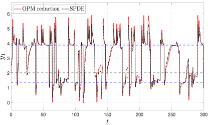
VII Towards the Reduction of More General Lévy-driven Dynamics
We prolong the discussion and results of Section VI towards more general Lévy noise. For the sake of simplicity we focus on finite-dimensional SDEs driven by Lévy processes.
There is a vast literature on Lévy processes which roughly speaking are processes given as the sum of a Brownian motion and a jump process [147, 148, 149, 150, 151]. Unlike the case of diffusion processes (SDEs driven by Brownian motions), the representation of Kolmogorov operators is non-unique in the case of Lévy-driven SDEs, and may take the form of operators involving fractional Laplacians or singular integrals among other representations [152]. We adopt here the definition commonly used in probability theory [153, Theorem 3.5.14] which presents the interest of being particularly intuitive as recalled below. We consider SDEs of the form
| (105) |
where is a Brownian motion in , and is a Lévy process on independent from . Here, we take to be a smooth vector field on , and to be, for each , a matrix with smooth entries, such that is a positive definite matrix for each in .
Roughly speaking, a Lévy process on is a non-Gaussian stochastic process with independent and stationary increments that experience sudden, large jumps in any direction. The probability distribution of the these jumps is characterized by a non-negative Borel measure defined on and concentrated on that satisfies the property . This measure is called the jump measure of the Lévy process . Sometimes itself is referred to as a Lévy process with triplet . Within this convention, we reserve ourselves the terminology of a Lévy process to a process with triplet . We refer to [149] and [148] for the mathematical background on Lévy processes.
Under suitable assumptions on , , and the Lévy measure , the solution to Eq. (105) is a Markov process (e.g. [154]) and even a Feller process [155], with associated Kolmogorov operator taking the following integro-differential form for (e.g.) in (Courrège theorem [156, 150]):
| (106) | ||||
where denotes the indicator function of the (open) unit ball in ; see also [149, Theorem 3.3.3].
The first-order term in Eq. (106) is the drift term caused by the deterministic, nonlinear dynamics. The second-order differential operator represents the diffusion part of the process . It is responsible for the continuous component of the process.
The -term, involving the integral, represents the jump part of the process. It captures the discontinuous jumps that the process experience due to the sudden changes caused by the Lévy process . Its intuitive interpretation breaks down as follows. The term, , calculates the difference in the test function value before and after the potential jump, capturing the change in the test function due to the jump.
The term represents a first-order correction for small jumps. It aims to account for the fact that a small jump might not land exactly on the grid point (), but somewhere in its vicinity. This term is often referred to as the Girsanov correction. Thus, the integral term accounts for all possible jump sizes () within a unit ball, as weighted by the Lévy measure . The notion of Kolmogorov operators can be extended to SPDEs driven by cylindrical Wiener processes, with lying in a Hilbert space; see [157]. Building up on such a functional framework, it is possible to provide a rigorous meaning of the Kolmogorov operator in the case of an SPDE driven by a general Lévy process, forcing possibly infinitely many modes.
In the case of SPDE driven by a scalar jump process (forcing only two modes) studied in Section VI (see Eq. (94)), the jump measure is simple to describe. It corresponds to the measure ( real) associated with the real-valued jump process given by Eq. (95). This measure is the Dirac delta , where is the intensity of the Poisson process associated with the random comb signal. Recall that this intensity is the limit of the probability of a single event occurring in a small interval divided by the length of that interval as the interval becomes infinitesimally small. Therefore, is equal to the firing rate of .
In the case of SDEs driven by -stable Lévy processes,
| (107) |
where the non-Gaussianity index lies in , and is a constant that depends on the dimension and involves the gamma function of Euler [152]. A -stable () process is simply a Brownian motion.

The rigorous theory of slow and center manifolds are in their infancy for SDEs driven by -stable Lévy processes [84, 158], but the main formulas share the same ingredients as recalled in Section II.2, with analogous backward-forward interpretations of those discussed in Section II.3 for the Lyapunov-Perron integrals involved therein ([84, Sec. 4]). The non-Markovian parameterizations of Section III and their data-driven optimization, can thus be extended, at least formally, for the case of SDEs driven by -stable Lévy processes and will be pursued elsewhere on concrete applications.
VIII A Chart Summarizing the Approach
To streamline the application of the OPM reduction approach for stochastically forced systems presented in this paper, we provide a concise overview of its key steps, objectives, and characteristics in the chart shown in Figure Fig. 16. This summary is tailored to the class of SPDEs discussed in Section II.1, with the primary goal of performing a reduction with a cutoff scale just below the forcing scale. This reduction involves a solution splitting where only the disregarded ”small” scales are stochastically forced (Figures 16A and 16B).
Given this splitting, where the disregarded scales are those directly forced by stochasticity, our approach reveals the importance of non-Markovian terms in the parameterization of these scales. These terms depend on the noise’s path history, enabling the tracking of small-scale fluctuations. The accuracy of this tracking is primarily governed by the memory content () of the parameterization, which is optimized from data by minimizing a natural loss function (Figure 16E) over a single noise realization .
Once optimized, the resulting non-Markovian parameterization, the Optimal Parameterizing Manifold (OPM), allows us to capture the average behavior of small-scale fluctuations as a functional of large scales by averaging over noise paths (see inset below Figure 16B). To efficiently optimize the memory content () and avoid the computation of cumbersome quadratures, we decompose the -term in Figure 16, , into random coefficients that solve simple auxiliary ODEs dependent on and the noise path . The resulting OPM closure, exemplified by Equation (85), takes the form of an SDE system with coefficients that are nonlinear functionals of these terms (Figure 16F) reflecting the nonlinear interactions between the noise and nonlinear terms in the original system.
As demonstrated with SPDEs driven by Gaussian noise (Section V) or jump processes (Section VI), the OPM closure effectively predicts noise-induced transitions and rare event statistics. This success is attributed to our hybrid approach, which combines analytical insights for constructing the parameterizing manifold (Figure 16C and Section III.1) with data-driven learning of the optimal memory content (Section III C).
IX Discussion and Perspectives
Thus, this work demonstrates that Optimal Parameterizing Manifolds (OPMs) constructed from Backward-Forward (BF) systems and optimized using a single solution path can accurately reproduce noise-induced transitions across a broad range of out-of-sample, test paths. This approach is effective for non-Gaussian noise with jumps. A remarkable feature of the approach is that, even though these two different types of noise typically lead to different dynamical responses, the OPMs in these two settings take exactly the same structural form with the corresponding non-Markovian terms depending on the past history of the corresponding noise forcing the original SPDE; cf. Eqns. (40)–(41) and cf Eqns. (99)–(100).
Interestingly, the optimal parameterization formulas align with the approximation of stochastic invariant manifolds when they exist. However, when these manifolds are no longer applicable, the optimal parameterizations transcends the invariance constraint. In such cases, it provides the optimal stochastic parameterization with respect to the random invariant measure (defined in Section IV.1), conditioned on the resolved variable (as proven in Theorem IV.1).
The formulas derived from the BF systems in Section III enable practical approximation of the theoretical optimal parameterization, particularly its non-Markovian random coefficients. These coefficients become crucial, especially when noise affects unresolved modes. They essentially encode how noise propagates to the resolved modes through nonlinear interactions.
We have shown, through various examples, that training on a single noise path equips the coefficients with an optimized historical memory (of the noise) that plays a key role in the accurate prediction of noise-induced excursion statistics, even when applied to a diverse set of test paths. This demonstrates the strength of our hybrid framework, which combines analytical understanding with data-driven insights. This approach allows us to overcome the “extrapolation problem,” a significant challenge for purely data-driven machine-learned parameterizations.
Section II.3 discusses the possibility of constructing more intricate parameterizations using an iterative scheme based on more general BF systems. However, these elaborations require more computational effort due to the repeated stochastic convolutions. Implementing them efficiently necessitates deriving auxiliary ODEs (analogues to Eq. (49)) for the coefficients ( and ) in Eqns. (31) and (32). Reference [29], Section 7.3, provides examples of such auxiliary ODEs for handling repeated stochastic convolutions.
These more general stochastic parameterizations have the potential to significantly enhance the parameterization capabilities of (Eq. (33)). This is because they encode higher-order interaction terms with respect to the noise amplitude, as shown in Eq. (30). Resolving these interactions is potentially important for improving the prediction of rare event statistics by non-Markovian reduced systems, especially when the noise intensity is low. This opens doors to potential applications using large deviation or rare event algorithms (e.g., [159, 160, 161, 162, 130, 163, 108, 21]). Additionally, iterating the BF system (Eq. (25)) beyond can also introduce higher-order terms involving the low-mode amplitude .
The inclusion of higher-term in is non-unique though. For instance, inspired by [29, Sec. 7.2.1], stochastic parameterizations accounting for higher-order terms in are produced by solving analytically the following BF system:
| (108) | ||||
for which the two first equations for and are simultaneously integrated backward over , followed by the forward integration of the -equation over the same interval. Compared to Eq. (LABEL:Eq_BF_SPDEcubic), this BF system has two-layer in the low-mode variable resulting into parameterizations of order 4 in ; see [164, Theorem 2] for an example. These higher-order terms come from the nonlinear self-interactions between the low modes as brought by the term . Accounting for additional interactions either through (LABEL:Eq_h2) or the iterative procedure of Section II.3 can help improve the parameterization skills (see also [103, 134]), and should be considered if accuracy is key to resolve.
An alternative route to enhance accuracy would involve to parameterize stochastically the parameterization residual from the loss functions in (53), post-minimization. This technique has proven effective in modeling the fast motion transversal to OPM manifolds by means of networks of nonlinear stochastic oscillators [47, 43], as diagnosed by Ruelle-Pollicott resonances [165, 166]. Similarly, rapid dynamical fluctuations, transversal to (Markovian) OPM manifolds (Figure 9), could benefit from refined parameterizations through the incorporation of additional stochastic components following [47], potentially leading to more accurate representation of rare event statistics by the corresponding closures (Figure 7).
Extending beyond SPDEs driven by Markov processes, our framework can naturally accommodate SPDEs driven by non-Markovian stochastic processes. A prime example is when the stochastic forcing is a fractional Brownian motion (fBm) [167], for which the existence of unstable manifolds has been demonstrated [168]. By leveraging Lyapunov-Perron techniques, as employed in the construction of these manifolds (Section II.2), our extension program to parameterization can proceed analogously to Section III. This involves here as well, finite-time integration of relevant backward-forward systems to derive optimizable parameterizations from the governing equation. The random coefficients in these parameterizations would then become again functionals of the past history of the forcing noise, albeit this time incorporating a higher degree of memory compared to the stochastic process used in the parameterizations Section III, due to the original memory content of the original forcing. Such generalized parameterizations should provide valuable insights into the interplay between nonlinearity and noise in physical systems exhibiting long-term memory effects [34, 35, 169].
Regardless of the Markovian or non-Markovian nature of the stochastic forcing, our reduction approach and its potential extensions offer valuable tools for addressing critical questions. By elucidating the intricate interplay between noise and nonlinearity, we can gain deeper dynamical insights. For example, we anticipate applying this reduction program to investigate early warning indicators of tipping phenomena, from a dynamical perspective, by tracing the energy flow from forced scales to physically relevant modes [170, 171]. Climate tipping elements provide a compelling domain for exploring these concepts and applying our methods [67, 172, 173].
The proposed stochastic parameterization method offers a new framework for understanding noise-nonlinearity interactions in stochastic multiscale systems. It is important to note that alternative techniques based on stochastic time scale separation, such as the stochastic path perturbation approach, have been employed to study related phenomena, including the random escape of stochastic fields from criticality in explosive systems [174] and first passage time problems in nonlocal Fisher equations [175, 176]. Future research directions could explore the potential of our method to obtain analytical approximations for first passage times in nonlocal SPDEs near criticality. Such an extension could provide valuable insights into pattern formations for a wide range of physical and biological problems such as in infectious disease modeling [177], nonlinear optics [178], or vegetation models [179].
Acknowledgements.
Several insights discussed in this work have substantially benefited from the reviewers’ constructive comments, and we express our deep gratitude to them. This work has been supported by the Office of Naval Research (ONR) Multidisciplinary University Research Initiative (MURI) grant N00014-20-1-2023, and by the National Science Foundation grants DMS-2108856, DMS-2407483, and DMS-2407484. This work has been also supported by the European Research Council (ERC) under the European Union’s Horizon 2020 research and innovation program (grant agreement No. 810370) and by a Ben May Center grant for theoretical and/or computational research.Appendix A Proof of Theorem II.1
Proof. Step 1. Let us remark that for any
where and .
Note that the product term above can be re-written as
| (109) | ||||
where and runs through the subsets (possibly empty) of disjoint elements of .
Thus,
| (110) | ||||
and by using (109), exists if and only if for each with , the integrals
| (111) |
exist as runs through the subsets (possibly empty) of disjoint elements of .
Since the OU process has sublinear growth (see e.g. [30, Lemma 3.1]), that is for all , one can readily check that the integral defined in (111) is finite for all provided that
| (112) |
Thus, the Lyapunov-Perron integral defined in Eq. (17) is well-defined if the non-resonance condition (LABEL:Eq_NR) holds.
Step 2. Thus is well defined under the condition (LABEL:Eq_NR). By direct calculation, we get
| (113) | ||||
and that
where denote the Fréchet derivative of . As a result, solves (19).
Appendix B Solving the sACE and its optimal reduced system
For the numerical integration of the stochastic Allen-Cahn equation (76), we adopt a semi-implicit Euler method, where the nonlinearity and the noise term are treated explicitly, and the linear term is treated implicitly; the spatial discretization is handled with a pseudo-spectral method; see [29, Section 6.1] for a detailed description of this scheme applied to a stochastic Burgers-type equation. We have set the time-step size to be and the spatial resolution to be .
The optimal reduced system (Eq. (85)) is also integrated with a semi-implicit Euler method where the linear term is treated implicitly and the nonlinear terms explicitly, still with . The ODEs with random coefficients such as (49), used to simulate the non-Markovian coefficients involved in the computation of , are simply integrated by a forward Euler scheme, with again . The initial condition (52) for integrating the RDE (49) is computed using the trapezoidal rule.
Appendix C Computations of the double-fold bifurcation diagram, and jump-induced transitions
C.1 Computation of the double-fold bifurcation diagram
To compute the double-fold bifurcation diagram shown in Figure 11 for Eq. (LABEL:Eq_Sbif), we adopt a Fourier sine series expansion of the solutions, in which solving Eq. (LABEL:Eq_Sbif) is approximated by . By doing so, the elliptic boundary value problem (LABEL:Eq_Sbif) is reduced to a nonlinear algebraic system for the coefficients , which is solved by the Matlab built-in solver fsolve. The results shown in Figure 11 are obtained from a six-dimensional algebraic system (i.e., with six sine modes, ), which turns out to provide high-precision approximations.
We use a simple continuation approach to compute the bifurcation diagram based on this algebraic system, benefiting from the knowledge that the solution curve is S-shaped. Starting from with a random initial guess, an increment of is used to compute the lower branch of solutions to Eq. (LABEL:Eq_Sbif) (lower black curve) with minimal energy. In our continuation procedure, the initial guess for is taken to be computed at the previous step. As is further increased, the procedure is stopped when the associated Jacobian becomes nearly singular which indicates that is approaching the lower turning point of the S-shaped curve.
The location of this turning point is estimated to be as obtained by using finer mesh as one gets close to singularity. We then select a -value to be just a few -increments below (to ensure multiplicity of solutions) and pick as many different random initial guesses as needed to get the two other solutions: the unstable one, , and the stable one, , with maximal energy. From each of these newly computed solutions, we then adopt the same continuation method to trace out the upper branch made of solutions with maximal energy (upper black curve) and the “in between” branch made of unstable solutions (red curve).
C.2 Solving the jump-driven dynamics in Eq. (97), and its optimal reduced model
The numerical integration of the stochastic equation (97) is performed in the same way as for the sACE outlined in Appendix B using a semi-implicit Euler method. Here also the nonlinearity and the noise term are treated explicitly, while the linear term is treated implicitly. The spatial discretization is handled with a pseudo-spectral method; see again [29, Section 6.1]. We have set the time-step size to be and the spatial resolution to be . The initial data is set to be for the results shown in Figs. 12 and 15.
The optimal reduced system (Eq. (LABEL:Eq_reduced_S_shaped)) is integrated with a forward Euler method still with . The initial condition (cf. (100)) for integrating (101) is computed using the trapezoidal rule, and . The initial data for Eq. (LABEL:Eq_reduced_S_shaped) is set to be the projection of the SPDE solution onto at time .
References
- [1] P. C. Hohenberg and B. I. Halperin, “Theory of dynamic critical phenomena,” Reviews of Modern Physics, vol. 49, no. 3, p. 435, 1977.
- [2] J. Pearson, “Complex patterns in a simple system,” Science, vol. 261, no. 5118, pp. 189–192, 1993.
- [3] M. Cross and P. Hohenberg, “Pattern formation outside of equilibrium,” Reviews of Modern Physics, vol. 65, no. 3, p. 851, 1993.
- [4] P. S. Berloff and J. C. McWilliams, “Large-scale, low-frequency variability in wind-driven ocean gyres,” Journal of Physical Oceanography, vol. 29, no. 8, pp. 1925–1949, 1999.
- [5] J. Murray, Mathematical Biology: II: Spatial Models and Biomedical Applications, vol. 3. Springer, 2003.
- [6] M. Baurmann, T. Gross, and U. Feudel, “Instabilities in spatially extended predator–prey systems: Spatio-temporal patterns in the neighborhood of Turing–Hopf bifurcations,” Journal of Theoretical Biology, vol. 245, no. 2, pp. 220–229, 2007.
- [7] F. Sagués, J. Sancho, and J. García-Ojalvo, “Spatiotemporal order out of noise,” Reviews of Modern Physics, vol. 79, no. 3, p. 829, 2007.
- [8] Y. R. Zelnik, E. Meron, and G. Bel, “Gradual regime shifts in fairy circles,” Proc. Natl. Acad. Sci., vol. 112, no. 40, pp. 12327–12331, 2015.
- [9] E. Meron, “From patterns to function in living systems: Dryland ecosystems as a case study,” Annual Review of Condensed Matter Physics, vol. 9, pp. 79–103, 2018.
- [10] J. McWilliams, “A survey of submesoscale currents,” Geoscience Letters, vol. 6, no. 1, pp. 1–15, 2019.
- [11] J. Crawford, “Introduction to bifurcation theory,” Reviews of Modern Physics, vol. 63, no. 4, p. 991, 1991.
- [12] T. Ma and S. Wang, Phase Transition Dynamics. Springer, second ed., 2019.
- [13] J. Crawford and E. Knobloch, “Symmetry and symmetry-breaking bifurcations in fluid dynamics,” Annual Review of Fluid Mechanics, vol. 23, no. 1, pp. 341–387, 1991.
- [14] M. D. Chekroun, E. Park, and R. Temam, “The Stampacchia maximum principle for stochastic partial differential equations and applications,” Journal of Differential Equation, vol. 260, no. 3, pp. 2926–2972, 2016.
- [15] H. Brand, S. Kai, and S. Wakabayashi, “External noise can suppress the onset of spatial turbulence,” Physical Review Letters, vol. 54, no. 6, p. 555, 1985.
- [16] S. Kai, H. Fukunaga, and H. R. Brand, “Structure changes induced by external multiplicative noise in the electrohydrodynamic instability of nematic liquid crystals,” Journal of statistical physics, vol. 54, pp. 1133–1152, 1989.
- [17] G. Ahlers, C. W. Meyer, and D. S. Cannell, “Deterministic and stochastic effects near the convective onset,” Journal of Statistical Physics, vol. 54, pp. 1121–1131, 1989.
- [18] J. García-Ojalvo, A. Hernández-Machado, and J. M. Sancho, “Effects of external noise on the Swift-Hohenberg equation,” Physical Review Letters, vol. 71, no. 10, p. 1542, 1993.
- [19] I. Rehberg, S. Rasenat, M. De La Torre Juarez, W. Schöpf, F. Hörner, G. Ahlers, and H. Brand, “Thermally induced hydrodynamic fluctuations below the onset of electroconvection,” Physical Review Letters, vol. 67, no. 5, p. 596, 1991.
- [20] P. Sura and C. Penland, “Sensitivity of a double-gyre ocean model to details of stochastic forcing,” Ocean Modelling, vol. 4, no. 3-4, pp. 327–345, 2002.
- [21] E. Simonnet, J. Rolland, and F. Bouchet, “Multistability and rare spontaneous transitions in barotropic -plane turbulence,” Journal of the Atmospheric Sciences, vol. 78, no. 6, pp. 1889–1911, 2021.
- [22] R. Saravanan and J. C. McWilliams, “Advective ocean–atmosphere interaction: An analytical stochastic model with implications for decadal variability,” Journal of Climate, vol. 11, no. 2, pp. 165–188, 1998.
- [23] M. S. Roulston and J. D. Neelin, “The response of an ENSO model to climate noise, weather noise and intraseasonal forcing,” Geophysical Research Letters, vol. 27, no. 22, pp. 3723–3726, 2000.
- [24] I. Eisenman, L. Yu, and E. Tziperman, “Westerly wind bursts: ENSO’s tail rather than the dog?,” Journal of Climate, vol. 18, no. 24, pp. 5224–5238, 2005.
- [25] G. Margazoglou, T. Grafke, A. Laio, and V. Lucarini, “Dynamical landscape and multistability of a climate model,” Proceedings of the Royal Society A, vol. 477, p. 20210019, 2021.
- [26] M. D. Chekroun, H. Liu, and J. C. McWilliams, “The emergence of fast oscillations in a reduced primitive equation model and its implications for closure theories,” Comp. & Fluids, vol. 151, pp. 3–22, 2017.
- [27] M. Chekroun, H. Liu, and J. McWilliams, “Variational approach to closure of nonlinear dynamical systems: Autonomous case,” J. Stat. Phys., vol. 179, no. 5, pp. 1073–1160, 2020. doi: 10.1007/s10955-019-02458-2.
- [28] M. Chekroun, H. Liu, and J. C. McWilliams, “Optimal parameterizing manifolds for anticipating tipping points and higher-order critical transitions,” Chaos, vol. 33, no. 9, 2023. doi.org/10.1063/5.0167419.
- [29] M. D. Chekroun, H. Liu, and S. Wang, Stochastic Parameterizing Manifolds and Non-Markovian Reduced Equations: Stochastic Manifolds for Nonlinear SPDEs II. Springer Briefs in Mathematics, Springer, 2015.
- [30] M. D. Chekroun, H. Liu, and S. Wang, Approximation of Stochastic Invariant Manifolds: Stochastic Manifolds for Nonlinear SPDEs I. Springer Briefs in Mathematics, Springer, 2015.
- [31] M. D. Chekroun, H. Liu, J. C. McWilliams, and S. Wang, “Transitions in stochastic non-equilibrium systems: Efficient reduction and analysis,” J. Diff. Eqns., vol. 346, pp. 145–204, 2023.
- [32] M. Schulz and M. Mudelsee, “REDFIT: estimating red-noise spectra directly from unevenly spaced paleoclimatic time series,” Computers & Geosciences, vol. 28, no. 3, pp. 421–426, 2002.
- [33] A. Moberg, D. M. Sonechkin, K. Holmgren, N. M. Datsenko, and W. Karlén, “Highly variable Northern Hemisphere temperatures reconstructed from low-and high-resolution proxy data,” Nature, vol. 433, no. 7026, pp. 613–617, 2005.
- [34] K. Fraedrich, R. Blender, and X. Zhu, “Continuum climate variability: Long-term memory, scaling, and 1/f-noise,” International Journal of Modern Physics B, vol. 23, no. 28n29, pp. 5403–5416, 2009.
- [35] M. Rypdal and K. Rypdal, “Long-memory effects in linear response models of Earth’s temperature and implications for future global warming,” Journal of Climate, vol. 27, no. 14, pp. 5240–5258, 2014.
- [36] M. Rypdal and K. Rypdal, “Late Quaternary temperature variability described as abrupt transitions on a 1/f noise background,” Earth System Dynamics, vol. 7, no. 1, pp. 281–293, 2016.
- [37] K. Hasselmann, “Stochastic climate models. Part I. Theory,” Tellus, vol. 28, no. 6, pp. 473–485, 1976.
- [38] J. W.-B. Lin and J. D. Neelin, “Influence of a stochastic moist convective parameterization on tropical climate variability,” Geophysical Research Letters, vol. 27, no. 22, pp. 3691–3694, 2000.
- [39] T. N. Palmer, “A nonlinear dynamical perspective on model error: A proposal for non-local stochastic-dynamic parametrization in weather and climate prediction models,” Quarterly Journal of the Royal Meteorological Society, vol. 127, no. 572, pp. 279–304, 2001.
- [40] A. J. Majda, I. Timofeyev, and E. Vanden-Eijnden, “A mathematical framework for stochastic climate models,” Comm. Pure Appl. Math, vol. 54, no. 8, pp. 891–974, 2001.
- [41] C. L. E. Franzke, T. J. O’Kane, J. Berner, P. D. Williams, and V. Lucarini, “Stochastic climate theory and modeling,” Wiley Interdisciplinary Reviews: Climate Change, vol. 6, no. 1, pp. 63–78, 2015.
- [42] J. Berner, U. Achatz, L. Batté, L. Bengtsson, A. Cámara, H. Christensen, M. Colangeli, D. Coleman, D. Crommelin, S. Dolaptchiev, C. Franzke, P. Friederichs, P. Imkeller, H. Järvinen, S. Juricke, V. Kitsios, F. Lott, V. Lucarini, S. Mahajan, T. Palmer, C. Penland, M. Sakradzija, J.-S. von Storch, A. Weisheimer, M. Weniger, P. Williams, and J.-I. Yano, “Stochastic Parameterization: Toward a New View of Weather and Climate Models,” Bull. Amer. Met. Soc., vol. 98, no. 3, pp. 565–588, 2017.
- [43] V. Lucarini and M. D. Chekroun, “Theoretical tools for understanding the climate crisis from Hasselmann’s programme and beyond,” Nature Reviews Physics, vol. 5, no. 12, pp. 744–765, 2023. doi:10.1038/s42254-023-00650-8.
- [44] A. J. Chorin, O. H. Hald, and R. Kupferman, “Optimal prediction with memory,” Physica D, vol. 166, no. 3, pp. 239–257, 2002.
- [45] D. Givon, R. Kupferman, and A. Stuart, “Extracting macroscopic dynamics: model problems and algorithms,” Nonlinearity, vol. 17, no. 6, pp. R55–R127, 2004.
- [46] P. Stinis, “A comparative study of two stochastic mode reduction methods,” Physica D, vol. 213, no. 2, pp. 197–213, 2006.
- [47] M. D. Chekroun, H. Liu, and J. C. McWilliams, “Stochastic rectification of fast oscillations on slow manifold closures,” Proc. Natl. Acad. Sci. USA, vol. 118, no. 48, p. e2113650118, 2021.
- [48] N. S. Namachchivaya and Y. K. Lin, “Method of stochastic normal forms,” Int. J. Non-linear Mechanics, vol. 26, no. 6, pp. 931–943, 1991.
- [49] P. H. Coullet, C. Elphick, and E. Tirapegui, “Normal form of a Hopf bifurcation with noise,” Phys. Lett. A, vol. 111, no. 6, pp. 277–282, 1985.
- [50] L. Arnold, Random Dynamical Systems. Springer, 1998.
- [51] E. Forgoston and I. B. Schwartz, “Escape rates in a stochastic environment with multiple scales,” SIAM J. Applied Dynamical Systems, vol. 8, no. 3, pp. 1190–1217, 2009.
- [52] D. Blömker and M. Hairer, Amplitude Equations for SPDEs: Approximate Centre Manifolds and Invariant Measures, in Probability and Partial Differential Equations in Modern Applied Mathematics, vol. 140 of IMA Vol. Math. Appl. Springer, New York, 2005.
- [53] D. Blömker, Amplitude Equations for Stochastic Partial Differential Equations, vol. 3 of Interdisciplinary Mathematical Science. World Scientific Publishing Co. Pte. Ltd., Hackensack, NJ, 2007.
- [54] D. Blömker, M. Hairer, and G. A. Pavliotis, “Multiscale analysis for stochastic partial differential equations with quadratic nonlinearities,” Nonlinearity, vol. 20, no. 7, pp. 1721–1744, 2007.
- [55] K. Klepel, D. Blömker, and W. W. Mohammed, “Amplitude equation for the generalized Swift–Hohenberg equation with noise,” Z. Angew. Math. Phys., vol. 65, pp. 1107–1126, 2014.
- [56] A. Bray, “Theory of phase-ordering kinetics,” Advances in Physics, vol. 51, no. 2, pp. 481–587, 2002.
- [57] U. C. Täuber, Critical dynamics: a Field Theory Approach to Equilibrium and Non-equilibrium Scaling Behavior. Cambridge University Press, 2014.
- [58] J. Bebernes and D. Eberly, Mathematical Problems from Combustion Theory, vol. 83. Springer Science & Business Media, 2013.
- [59] D. A. Frank-Kamenetskii, Diffusion and Heat Exchange in Chemical Kinetics. Princeton University Press, 2015.
- [60] H. Grad and H. Rubin, “Hydromagnetic equilibria and force-free fields,” Journal of Nuclear Energy, vol. 7, no. 3-4, pp. 284–285, 1958.
- [61] V. Shafranov, “On magnetohydrodynamical equilibrium configurations,” Soviet Journal of Experimental and Theoretical Physics, vol. 6, 1958.
- [62] E. M. Izhikevich, Dynamical Systems in Neuroscience: The Geometry of Excitability and Bursting. Cambridge: MIT Press, 2010.
- [63] M. Ghil, “Climate stability for a Sellers-type model,” Journal of the Atmospheric Sciences, vol. 33, no. 1, pp. 3–20, 1976.
- [64] G. R. North, R. F. Cahalan, and J. A. Coakley Jr, “Energy balance climate models,” Reviews of Geophysics, vol. 19, pp. 91–121, 1981.
- [65] O. Thual and J. Mcwilliams, “The catastrophe structure of thermohaline convection in a two-dimensional fluid model and a comparison with low-order box models,” Geophysical & Astrophysical Fluid Dynamics, vol. 64, no. 1-4, pp. 67–95, 1992.
- [66] W. Weijer, W. Cheng, S. Drijfhout, A. Fedorov, A. Hu, L. Jackson, W. Liu, E. McDonagh, J. Mecking, and J. Zhang, “Stability of the Atlantic Meridional Overturning Circulation: A review and synthesis,” Journal of Geophysical Research: Oceans, vol. 124, no. 8, pp. 5336–5375, 2019.
- [67] T. M. Lenton, H. Held, E. Kriegler, J. W. Hall, W. Lucht, S. Rahmstorf, and H. J. Schellnhuber, “Tipping elements in the earth’s climate system,” Proceedings of the national Academy of Sciences, vol. 105, no. 6, pp. 1786–1793, 2008.
- [68] N. Boers, “Observation-based early-warning signals for a collapse of the atlantic meridional overturning circulation,” Nature Climate Change, vol. 11, no. 8, pp. 680–688, 2021.
- [69] N. Boers and M. Rypdal, “Critical slowing down suggests that the western greenland ice sheet is close to a tipping point,” Proceedings of the National Academy of Sciences, vol. 118, no. 21, p. e2024192118, 2021.
- [70] N. Wunderling, J. F. Donges, J. Kurths, and R. Winkelmann, “Interacting tipping elements increase risk of climate domino effects under global warming,” Earth System Dynamics, vol. 12, no. 2, pp. 601–619, 2021.
- [71] L. Serdukova, Y. Zheng, J. Duan, and J. Kurths, “Metastability for discontinuous dynamical systems under Lévy noise: Case study on Amazonian Vegetation,” Scientific reports, vol. 7, no. 1, p. 9336, 2017.
- [72] Y. Zheng, F. Yang, J. Duan, X. Sun, L. Fu, and J. Kurths, “The maximum likelihood climate change for global warming under the influence of greenhouse effect and Lévy noise,” Chaos, vol. 30, no. 1, 2020.
- [73] P. Ditlevsen, “Observation of -stable noise induced millennial climate changes from an ice-core record,” Geophysical Research Letters, vol. 26, no. 10, pp. 1441–1444, 1999.
- [74] T. Solomon, E. R. Weeks, and H. L. Swinney, “Observation of anomalous diffusion and Lévy flights in a two-dimensional rotating flow,” Physical Review Letters, vol. 71, no. 24, p. 3975, 1993.
- [75] B. Khouider, A. Majda, and M. Katsoulakis, “Coarse-grained stochastic models for tropical convection and climate,” Proc. Natl. Acad. Sci. USA, vol. 100, no. 21, pp. 11941–11946, 2003.
- [76] S. N. Stechmann and J. D. Neelin, “A stochastic model for the transition to strong convection,” J. Atmos. Sci., vol. 68, no. 12, pp. 2955–2970, 2011.
- [77] C. Penland and P. Sardeshmukh, “Alternative interpretations of power-law distributions found in nature,” Chaos, vol. 22, no. 2, p. 023119, 2012.
- [78] S. Thual, A. J. Majda, N. Chen, and S. N. Stechmann, “Simple stochastic model for El Niño with westerly wind bursts,” Proceedings of the National Academy of Sciences, vol. 113, no. 37, pp. 10245–10250, 2016.
- [79] N. Chen and A. J. Majda, “Simple stochastic dynamical models capturing the statistical diversity of El Niño Southern Oscillation,” Proceedings of the National Academy of Sciences, vol. 114, no. 7, pp. 1468–1473, 2017.
- [80] N. Chen, C. Mou, L. M. Smith, and Y. Zhang, “A stochastic precipitating quasi-geostrophic model,” arXiv preprint arXiv:2407.20886, 2024.
- [81] I. Horenko, “Nonstationarity in multifactor models of discrete jump processes, memory, and application to cloud modeling,” Journal of the Atmospheric Sciences, vol. 68, no. 7, pp. 1493–1506, 2011.
- [82] M. D. Chekroun, I. Koren, H. Liu, and H. Liu, “Generic generation of noise-driven chaos in stochastic time delay systems: Bridging the gap with high-end simulations,” Science Advances, vol. 8, no. 46, p. eabq7137, 2022.
- [83] A. Debussche, M. Högele, and P. Imkeller, The Dynamics of Nonlinear Reaction-diffusion Equations with Small Lévy Noise, vol. 2085. Springer, 2013.
- [84] S. Yuan, J. Hu, X. Liu, and J. Duan, “Slow manifolds for dynamical systems with non-Gaussian stable Lévy noise,” Analysis and Applications, vol. 17, no. 03, pp. 477–511, 2019.
- [85] X. Liu, “Random invariant manifolds of stochastic evolution equations driven by Gaussian and non-Gaussian noises,” Journal of Mathematical Physics, vol. 62, no. 11, p. 112702, 2021.
- [86] S. Yuan and D. Bloemker, “Modulation and amplitude equations on bounded domains for nonlinear SPDEs driven by cylindrical -stable Lévy processes,” SIAM Journal on Applied Dynamical Systems, vol. 21, no. 3, pp. 1748–1777, 2022.
- [87] G. Da Prato and J. Zabczyk, Stochastic Equations in Infinite Dimensions, vol. 44 of Encyclopedia of Mathematics and its Applications. Cambridge: Cambridge University Press, 2008.
- [88] G. Da Prato and J. Zabczyk, Ergodicity for Infinite Dimensional Systems. Cambridge University Press, 1996.
- [89] D. Henry, Geometric Theory of Semilinear Parabolic Equations, vol. 840 of Lecture Notes in Mathematics. Springer-Verlag, Berlin, 1981.
- [90] A. Pazy, Semigroups of Linear Operators and Applications to Partial Differential Equations, vol. 44 of Applied Mathematical Sciences. Springer-Verlag, New York, 1983.
- [91] T. Ma and S. Wang, Bifurcation Theory and Applications, vol. 53 of World Scientific Series on Nonlinear Science. Series A: Monographs and Treatises. World Scientific Publishing Co. Pte. Ltd., Hackensack, NJ, 2005.
- [92] G. J. Lord, C. E. Powell, and T. Shardlow, An Introduction to Computational Stochastic PDEs, vol. 50. Cambridge University Press, 2014.
- [93] M. D. Chekroun and H. Liu, “Effective reduced models from delay differential equations: Bifurcations, tipping solution paths, and ENSO variability,” Physica D, vol. 460, p. 134058, 2024.
- [94] K.-J. Engel and R. Nagel, One-Parameter Semigroups for Linear Evolution Equations, vol. 194 of Graduate Texts in Mathematics. New York: Springer-Verlag, 2000.
- [95] M. Chekroun, H. Dijkstra, T. Sengül, and S. Wang, “Transitions of zonal flows in a two-layer quasi-geostrophic ocean model,” Nonlinear dynamics, vol. 109, no. 3, pp. 1887–1904, 2022.
- [96] A. Bensoussan and F. Flandoli, “Stochastic inertial manifold,” Stochastics Stochastics Rep., vol. 53, pp. 13–39, 1995.
- [97] G. Da Prato and A. Debussche, “Construction of stochastic inertial manifolds using backward integration,” Stochastics Stochastics Reports, vol. 59, no. 3-4, pp. 305–324, 1996.
- [98] G. Jetschke, “On the equivalence of different approaches to stochastic partial differential equations,” Mathematische Nachrichten, vol. 128, no. 1, pp. 315–329, 1986.
- [99] I. Corwin, “The Kardar–Parisi–Zhang equation and universality class,” Random matrices: Theory and applications, vol. 1, no. 01, p. 1130001, 2012.
- [100] A. J. Roberts, “A step towards holistic discretisation of stochastic partial differential equations,” ANZIAM Journal, vol. 45, pp. C1–C15, 2003.
- [101] A. J. Roberts, “Resolving the multitude of microscale interactions accurately models stochastic partial differential equations,” LMS Journal of Computation and Mathematics, vol. 9, pp. 193–221, 2006.
- [102] W. Wang and A. Roberts, “Macroscopic reduction for stochastic reaction–diffusion equations,” The IMA Journal of Applied Mathematics, vol. 78, no. 6, pp. 1237–1264, 2013.
- [103] D. Blömker and W. W. Mohammed, “Amplitude equations for SPDEs with cubic nonlinearities,” Stochastics: An International Journal of Probability and Stochastic Processes, vol. 85, no. 2, pp. 181–215, 2013.
- [104] J. Cahn and J. Hilliard, “Free energy of a nonuniform system. I. Interfacial free energy,” The Journal of chemical physics, vol. 28, no. 2, pp. 258–267, 1958.
- [105] G. Da Prato and A. Debussche, “Stochastic Cahn-Hilliard equation,” Nonlinear Analysis: Theory, Methods & Applications, vol. 26, no. 2, pp. 241–263, 1996.
- [106] S. Pierini, “Coherence resonance in a double-gyre model of the Kuroshio Extension,” Journal of Physical Oceanography, vol. 40, no. 1, pp. 238–248, 2010.
- [107] T. P. Sapsis and H. A. Dijkstra, “Interaction of additive noise and nonlinear dynamics in the double-gyre wind-driven ocean circulation,” Journal of physical oceanography, vol. 43, no. 2, pp. 366–381, 2013.
- [108] V. M. Gálfi, V. Lucarini, F. Ragone, and J. Wouters, “Applications of large deviation theory in geophysical fluid dynamics and climate science,” La Rivista del Nuovo Cimento, vol. 44, no. 6, pp. 291–363, 2021.
- [109] M. Hairer and J. Mattingly, “A theory of hypoellipticity and unique ergodicity for semilinear stochastic PDEs,” Electron. J. Probab., pp. 658–738, 2011.
- [110] M. Hairer and A. Ohashi, “Ergodic theory for SDEs with extrinsic memory,” Ann. Probab., pp. 1950–1977, 2007.
- [111] B. Øksendal, Stochastic Differential Equations: An Introduction with Applications. Springer, 2013.
- [112] B. Goldys and B. Maslowski, “Exponential ergodicity for stochastic Burgers and 2D Navier–Stokes equations,” Journal of Functional Analysis, vol. 226, no. 1, pp. 230–255, 2005.
- [113] S. Kuksin and A. Shirikyan, Mathematics of Two-Dimensional Turbulence, vol. 194. Cambridge University Press, 2012.
- [114] M. Hairer and J. Mattingly, “Ergodicity of the 2D Navier-Stokes equations with degenerate stochastic forcing,” Annals of Mathematics, pp. 993–1032, 2006.
- [115] M. Hairer, J. Mattingly, and M. Scheutzow, “Asymptotic coupling and a general form of Harris theorem with applications to stochastic delay equations,” Probability Theory and Related Fields, vol. 149, no. 1-2, pp. 223–259, 2011.
- [116] M. Hairer, “Exponential mixing properties of stochastic PDEs through asymptotic coupling,” Probability theory and related fields, vol. 124, no. 3, pp. 345–380, 2002.
- [117] H. Crauel, “Measure attractors and Markov attractors,” Dynamical Systems, vol. 23, no. 1, pp. 75–107, 2008.
- [118] F. Flandoli, B. Gess, and M. Scheutzow, “Synchronization by noise for order-preserving random dynamical systems,” The Annals of Probability, vol. 45, no. 2, pp. 1325–1350, 2017.
- [119] H. Crauel, “Markov measures for random dynamical systems,” Stochastics: An International Journal of Probability and Stochastic Processes, vol. 37, no. 3, pp. 153–173, 1991.
- [120] H. Crauel, Random Probability Measures on Polish Spaces, vol. 11. The Stochastic Monographs: Theory and Applications of Stochastic Process Series, Taylor & Francis, 2002.
- [121] I. Chueshov, Monotone Random Systems Theory and Applications, vol. 1779. Springer Science & Business Media, 2002.
- [122] H. Crauel and F. Flandoli, “Attractors for random dynamical systems,” Probab. Theory Relat. Fields, vol. 100, pp. 365–393, 1994.
- [123] H. Brézis, Functional Analysis, Sobolev Spaces and Partial Differential Equations. Springer, 2010.
- [124] M. D. Chekroun, J. S. W. Lamb, C. J. Pangerl, and M. Rasmussen, “A Girsanov approach to slow parameterizing manifolds in the presence of noise,” arXiv preprint 1903.08598, 2023.
- [125] S. M. Allen and J. W. Cahn, “A microscopic theory for antiphase boundary motion and its application to antiphase domain coarsening,” Acta Metallurgica, vol. 27, no. 6, pp. 1085–1095, 1979.
- [126] N. Chafee and E. F. Infante, “A bifurcation problem for a nonlinear partial differential equation of parabolic type,” Applicable Analysis, vol. 4, no. 1, pp. 17–37, 1974.
- [127] V. Ginzburg and L. Landau, “On the theory of superconductivity,” Zh. Eksp. Teor. Fiz., vol. 20, pp. 1064–1082, 1950.
- [128] M. I. Freidlin and A. D. Wentzell, Random Perturbations of Dynamical Systems, vol. 260 of Grundlehren der Mathematischen Wissenschaften. Heidelberg: Springer, third ed., 2012. Translated from the 1979 Russian original by Joseph Szücs.
- [129] N. Berglund and B. Gentz, “Sharp estimates for metastable lifetimes in parabolic SPDEs: Kramers’ law and beyond,” Electron. J. Probab., vol. 18, pp. 1–58, 2013.
- [130] J. Rolland, F. Bouchet, and E. Simonnet, “Computing transition rates for the 1-D stochastic Ginzburg-Landau-Allen-Cahn equation for finite-amplitude noise with a rare event algorithm,” Journal of Statistical Physics, vol. 162, pp. 277–311, 2016.
- [131] R. Zakine and E. Vanden-Eijnden, “Minimum-action method for nonequilibrium phase transitions,” Physical Review X, vol. 13, no. 4, p. 041044, 2023.
- [132] T. Caraballo, H. Crauel, J. A. Langa, and J. C. Robinson, “The effect of noise on the Chafee-Infante equation: A nonlinear case study,” Proc. Amer. Math. Soc., vol. 135, no. 2, pp. 373–382, 2007.
- [133] D. Blömker and H. Fu, “The impact of multiplicative noise in SPDEs close to bifurcation via amplitude equations,” Nonlinearity, vol. 33, no. 8, p. 3905, 2020.
- [134] S. Qu and H. Gao, “The high-order approximation of SPDEs with multiplicative noise via amplitude equations,” Communications in Nonlinear Science and Numerical Simulation, 2024. 10.1016/j.cnsns.2024.107937.
- [135] F. Bai, A. Spence, and A. M. Stuart, “The numerical computation of heteroclinic connections in systems of gradient partial differential equations,” SIAM J. Appl. Math., vol. 53, no. 3, pp. 743–769, 1993.
- [136] W. W. Mohammed, D. Blömker, and K. Klepel, “Multi-scale analysis of SPDEs with degenerate additive noise,” J. Evolution Equations, vol. 14, pp. 273–298, 2014.
- [137] S. Chandrasekhar, An Introduction to the Study of Stellar Structure. Dover Publ., N. Y., 1957.
- [138] R. H. Fowler, “Further studies of Emden’s and similar differential equations,” The Quarterly Journal of Mathematics, no. 1, pp. 259–288, 1931.
- [139] E. Hopf, “On Emden’s differential equation,” Monthly Notices of the Royal Astronomical Society, vol. 91, 1931.
- [140] G. Hetzer, “S-shapedness for energy balance climate models of Sellers-type,” in The Mathematics of Models for Climatology and Environment, pp. 253–287, Springer, 1997.
- [141] H. Dijkstra and M. Moleamaker, “Symmetry breaking and overturning oscillations in thermohaline-driven flows,” Journal of Fluid Mechanics, vol. 331, pp. 169–198, 1997.
- [142] P. Korman and Y. Li, “On the exactness of an S-shaped bifurcation curve,” Proceedings of the American Mathematical Society, vol. 127, no. 4, pp. 1011–1020, 1999.
- [143] L. N. Trefethen, Spectral methods in MATLAB. SIAM, 2000.
- [144] I. Bena, “Dichotomous Markov noise: exact results for out-of-equilibrium systems,” International Journal of Modern Physics B, vol. 20, no. 20, pp. 2825–2888, 2006.
- [145] W. Horsthemke and R. Lefever, Noise-induced Transitions in Physics, Chemistry, and Biology. Springer, 1984.
- [146] Note that the other unresolved (and unforced) modes contain less than of the total energy and are thus not taken here in account into the parameterization .
- [147] R. Cont and P. Tankov, Financial Modelling with Jump Processes. Chapman and Hall/CRC, 2003.
- [148] S. Peszat and J. Zabczyk, Stochastic Partial Differential Equations with Lévy noise: An Evolution Equation approach, vol. 113. Cambridge University Press, 2007.
- [149] D. Applebaum, “Levy Processes and Stochastic Calculus,” Cambridge Studies in Advanced Mathematics, vol. 116, 2009.
- [150] F. Kühn, “Lévy Matters. VI,” Lecture Notes in Mathematics, vol. 2187, 2017.
- [151] B. Øksendal and A. Sulem, “Stochastic Control of Jump Diffusions,” in Applied Stochastic Control of Jump Diffusions, pp. 93–155, Springer, 2019.
- [152] M. Kwaśnicki, “Ten equivalent definitions of the fractional Laplace operator,” Fractional Calculus and Applied Analysis, vol. 20, no. 1, pp. 7–51, 2017.
- [153] D. Applebaum, Semigroups of Linear Operators: With Applications to Analysis, Probability and Physics. London Mathematical Society Student Texts, Cambridge University Press, 2019. doi:10.1017/9781108672641.
- [154] P. E. Protter, “Stochastic Integration and Differential Equations,” in Stochastic Modelling and Applied Probability, Springer, 2005.
- [155] F. Kühn, “Solutions of Lévy-driven SDEs with unbounded coefficients as Feller processes,” Proceedings of the American Mathematical Society, vol. 146, no. 8, pp. 3591–3604, 2018.
- [156] P. Courrège, “Sur la forme intégro-différentielle des opérateurs de dans satisfaisant au principe du maximum,” Séminaire Brelot-Choquet-Deny. Théorie du Potentiel, vol. 10, no. 1, pp. 1–38, 1965.
- [157] G. Da Prato, Kolmogorov Equations for Stochastic PDEs. Springer Science & Business Media, 2004.
- [158] S. Yuan, Z. Zeng, and J. Duan, “Stochastic bifurcation for two-time-scale dynamical system with -stable Lévy noise,” Journal of Statistical Mechanics: Theory and Experiment, vol. 2021, no. 3, p. 033204, 2021.
- [159] W. E, W. Ren, and E. Vanden-Eijnden, “Minimum action method for the study of rare events,” Communications on Pure and Applied Mathematics, vol. 57, pp. 637–656, 2004.
- [160] F. Cérou and A. Guyader, “Adaptive multilevel splitting for rare event analysis,” Stochastic Analysis and Applications, vol. 25, no. 2, pp. 417–443, 2007.
- [161] E. Vanden-Eijnden and M. G. Westdickenberg, “Rare events in stochastic partial differential equations on large spatial domains,” J. Stat. Phys., vol. 131, no. 6, pp. 1023–1038, 2008.
- [162] T. Grafke, R. Grauer, and T. Schäfer, “The instanton method and its numerical implementation in fluid mechanics,” Journal of Physics A: Mathematical and Theoretical, vol. 48, no. 33, p. 333001, 2015.
- [163] F. Ragone, J. Wouters, and F. Bouchet, “Computation of extreme heat waves in climate models using a large deviation algorithm,” Proceedings of the National Academy of Sciences, vol. 115, no. 1, pp. 24–29, 2018.
- [164] M. D. Chekroun and H. Liu, “Finite-horizon parameterizing manifolds, and applications to suboptimal control of nonlinear parabolic PDEs,” Acta Applicandae Mathematicae, vol. 135, no. 1, pp. 81–144, 2015.
- [165] M. D. Chekroun, A. Tantet, H. Dijkstra, and J. D. Neelin, “Ruelle-Pollicott resonances of stochastic systems in reduced state space. Part I: Theory,” J. Stat. Phys., vol. 179, pp. 1366–1402, 2020. doi: 10.1007/s10955-020-02535-x.
- [166] A. Tantet, M. D. Chekroun, H. Dijkstra, and J. D. Neelin, “Ruelle-Pollicott resonances of stochastic systems in reduced state space. Part II: stochastic Hopf bifurcation,” J. Stat. Phys., vol. 179, pp. 1403–1448, 2020. doi:10.1007/s10955-020-02526-y.
- [167] B. B. Mandelbrot and J. W. Van Ness, “Fractional Brownian motions, fractional noises and applications,” SIAM Review, vol. 10, no. 4, pp. 422–437, 1968.
- [168] M. J. Garrido-Atienza, K. Lu, and B. Schmalfuß, “Unstable invariant manifolds for stochastic PDEs driven by a fractional Brownian motion,” Journal of Differential Equations, vol. 248, no. 7, pp. 1637–1667, 2010.
- [169] M. Pereira, C. Gissinger, and S. Fauve, “1/f noise and long-term memory of coherent structures in a turbulent shear flow,” Physical Review E, vol. 99, p. 023106, 2019.
- [170] R. M. van Westen, M. Kliphuis, and H. A. Dijkstra, “Physics-based early warning signal shows that AMOC is on tipping course,” Science Advances, vol. 10, p. eadk1189, 2024.
- [171] V. Lucarini and M. Chekroun, “Detecting and attributing change in climate and complex Systems: Foundations, Green’s functions, and nonlinear fingerprints,” Physical Review Letters, vol. 133, p. 224201, 2024. doi:10.1103/PhysRevLett.133.244201.
- [172] T. M. Lenton, J. Rockström, O. Gaffney, S. Rahmstorf, K. Richardson, W. Steffen, and H. J. Schellnhuber, “Climate tipping points—too risky to bet against,” Nature, vol. 575, pp. 592–595, 2019.
- [173] D. I. A. McKay, A. Staal, J. F. Abrams, R. Winkelmann, B. Sakschewski, S. Loriani, I. Fetzer, S. E. Cornell, J. Rockström, and T. M. Lenton, “Exceeding 1.5∘C global warming could trigger multiple climate tipping points,” Science, vol. 377, p. eabn7950, 2022.
- [174] M. O. Cáceres and M. A. Fuentes, “Stochastic escape processes from a non-symmetric potential normal form III: extended explosive systems,” Journal of Physics A: Mathematical and General, vol. 32, no. 18, p. 3209, 1999.
- [175] M. Fuentes, M. Kuperman, and V. Kenkre, “Nonlocal interaction effects on pattern formation in population dynamics,” Physical Review Letters, vol. 91, p. 158104, 2003.
- [176] M. O. Cáceres and M. A. Fuentes, “First-passage times for pattern formation in nonlocal partial differential equations,” Physical Review E, vol. 92, p. 042122, 2015.
- [177] S. Ruan, “Spatial-temporal dynamics in nonlocal epidemiological models,” in Mathematics for Life Science and Medicine, Takeuchi, Y., Iwasa, Y., Sato, K. (eds), pp. 97–122, Springer, 2007.
- [178] C. Fernandez-Oto, M. Clerc, D. Escaff, and M. Tlidi, “Strong nonlocal coupling stabilizes localized structures: an analysis based on front dynamics,” Physical Review Letters, vol. 110, p. 174101, 2013.
- [179] E. Gilad, J. von Hardenberg, A. Provenzale, M. Shachak, and E. Meron, “Ecosystem engineers: from pattern formation to habitat creation,” Physical Review Letters, vol. 93, p. 098105, 2004.