Non-linear equation in the re-summed next-to-leading order of perturbative QCD:
the leading twist approximation
Abstract
In this paper, we use the re-summation procedure, suggested in Refs.DIMST ; SALAM ; SALAM1 ; SALAM2 , to fix the BFKL kernel in the NLO. However, we suggest a different way to introduce the non-linear corrections in the saturation region, which is based on the leading twist non-linear equation. In the kinematic region: , where denotes the size of the dipole, its rapidity and the saturation scale, we found that the re-summation contributes mostly to the leading twist of the BFKL equation. Assuming that the scattering amplitude is small, we suggest using the linear evolution equation in this region. For we are dealing with the re-summation of and other corrections in NLO approximation for the leading twist. We find the BFKL kernel in this kinematic region and write the non-linear equation, which we solve analytically. We believe the new equation could be a basis for a consistent phenomenology based on the CGC approach.
pacs:
12.38.Cy, 12.38g,24.85.+p,25.30.HmI Introduction
The Colour Glass Condensate(CGC) approach is the only candidate for an effective theory at high energies, which is based on our microscopic theory: QCD (see Ref.KOLEB for a review). However, it has been known for a long time, that to describe the scattering amplitude in the framework of CGCJIMWLK1 ; JIMWLK2 ; JIMWLK3 ; JIMWLK4 ; JIMWLK5 ; JIMWLK6 ; BK we need to include at least the next-to-leading order corrections to the non-linear equations. Indeed, the two essential parameters, that determine the high energy scattering, are the BFKL PomeronBFKL intercept, which is equal to , which leads to the energy behaviour of the scattering amplitude , and the energy behaviour of the new dimensional scale: saturation momentum . Both show the increase in the leading order CGC approach, which cannot be reconciled with the available experimental data. So, the large NLO corrections appear as the only way out, now as well as two decades ago.
The non-linear equations in the NLO has been written in Refs.NLOBK0 ; NLOBK01 ; NLOBK1 ; NLOBK2 ; JIMWLKNLO1 ; JIMWLKNLO2 ; JIMWLKNLO3 ; DIMST , but their use in high energy phenomenology is marred by the instabilities due to the presence of large and negative NLO corrections enhanced by double collinear logarithms (see Ref.DIMST for discussions and references). These problems have been found in Refs.BFKLNLO ; BFKLNLO1 , identified and solved in Refs.SALAM ; SALAM1 ; SALAM2 for the linear BFKL equation. It turns out that instabilities are closely related to the wrong choice of the energy(rapidity) scale, and we need to introduce the re-summed NLO corrections to cure this problem.
In this paper, we use the re-summation procedure, suggested in Refs.SALAM ; SALAM1 ; SALAM2 , to fix the BFKL kernel in the NLO, which coincides with the kernel used in Ref.DIMST . However, we suggest a different way to introduce the non-linear corrections, than in Ref.DIMST , which is based on the approach, developed in Ref.LETU for the leading twist non-linear equation in the LO. Our first observation is that the re-summation contributes mostly to the leading twist of the BFKL equation in the kinematic region , where denotes the size of the dipole, its rapidity and the saturation scale. We assume that at the scattering amplitude is small and we can neglect the non-linear corrections. Therefore, for we can restrict ourselves by the linear BFKL equation. For we are dealing with the re-summation of and other corrections in NLO approximation for the leading twist. In this paper we find the BFKL kernel in this kinematic region, and write the non-linear equation. We found the analytical solution of this equation, and believe the new equation could be a basis for a consistent phenomenology based on the CGC approach.
II BK non -linear equation
The BK evolution equation for the dipole-target scattering amplitude has in the leading order (LO) of perturbative QCDKOLEB ; BK ; GLR ; MUQI ; MV the following form:
| (1) |
where and , and . is the rapidity of the scattering dipole and is the impact factor. is the kernel of the BFKL equation which in the leading order has the following form:
| (2) |
In Eq. (II) denotes the size of the target dipole and where is the number of colours.
| (3) |
where denotes the Euler psi-function .
In the next-to-leading order (NLO), the non-linear equation has a more complicated formNLOBK0 ; NLOBK01 ; NLOBK1 ; NLOBK2 :
| (4) |
In Eq. (II) , denotes the renormalization scale for the running QCD coupling, and and are the number of fermions and colours, respectively. denotes the S-matrix for scattering of a dipole of size with the target, which can be written using the scattering amplitude , as follows . Eq. (II) gives the explicit form of the BFKL kernel in the NLO, but as it has been alluded to we need to re-sum the NLO corrections to avoid instabilities. We re-sum in the approximation, that was suggested in Ref.DIMST , which we will discuss below. It turns out, that in the framework of this re-summation we can neglect the contribution, which is proportional to in Eq. (II); and reduce Eq. (II) to Eq. (II) with the kernel, which has to be found in the re-summed NLO. An additional argument for such simplification stems from the fact that deep in the saturation region, where , all terms except the first one, which is proportional to , are small and can be neglected. In other words, deep in the saturation region Eq. (II) reduces to Eq. (II) without addressing the specific form of re-summation.
In the next-to-leading order the kernel is derived in Refs.BFKLNLO ; BFKLNLO1 and has the following form:
| (5) |
The explicit form of is given in Ref.BFKLNLO . However, turns out to be singular at , . Such singularities indicate, that we have to calculate higher order corrections to obtain a reliable result. The procedure to re-sum high order corrections is suggested in Ref. SALAM ; SALAM1 ; SALAM2 ; KMRS . The resulting spectrum of the BFKL equation in the NLO, can be found from the solution of the following equation SALAM ; SALAM1 ; SALAM2
| (6) |
where
| (7) |
and
| (8) | |||
Functions and as well as the constants ( and ), are defined in Refs.SALAM ; SALAM1 ; SALAM2 .
In Ref. KMRS Khoze, Martin, Ryskin and Stirling (KMRS) sugested an economic form of , which coincides with Eq. (8) to within , and, therefore, gives reasonable estimates of all constants and functions in Eq. (8). The equation for takes the form
| (9) |
One can see that when as follows from energy conservation.
III NLO BFKL kernel in the perturbative QCD region
III.1 Eigenfunctions of the BFKL equation
Therefore, the linear BFKL equation in the NLO takes the form:
| (10) |
The general solution to Eq. (10) can be written as follows
| (11) |
where is the eigenfunction of the BFKL equation and can be found from the initial condition at . In Eq. (11) denotes the size of the scattering dipole, while the size of the target.
In Ref.LIP it was proved that the eigenfunction of the BFKL equation has the following form
| (12) | |||||
| (13) |
for any kernel, which satisfies the conformal symmetry. Using Eq. (12) we can re-write the general solution in the form:
| (14) |
where . Comparing Eq. (13) with this definition of , one can see that
| (15) |
for .
III.2 Eigenvalues of the BFKL equation
As has been mentioned, the re-summation, that has been suggested in Ref.DIMST is determined by the anomalous dimension in the vicinity of the eigenvalues at . The singular part of the general kernel in the NLO (see Eq. (6)) has the following form:
| (16) |
with the solution:
| (17) |
It is instructive to note that Eq. (9) gives
| (18) |


III.3 Saturation and geometric scaling behaviour of the scattering amplitude in the NLO
It is well knownKOLEB ; GLR ; BALE ; LETU ; IIML ; MUT , that one does not need to know the precise structure of the non-linear corrections for finding the saturation momentum, as well as for discussing the behaviour of the scattering amplitude in the vicinity of the saturation scale. We only need to find the solution of the linear BFKL equation, which is a wave package that satisfies the condition, that phase and group velocities are equalGLR . This solution determines the new dimensional scale of the problem: the saturation momentum . The equation takes the form
| (20) |
For the eigenvalues of the BFKL equation in the NLO given by Eq. (17), the solution to Eq. (20) takes the form:
| (21) |
The equation
| (22) |
determines the saturation momentum 111Actually depends on other variables as well (see Eq. (15)), but we will omit these variable in the further presentation..
For Eq. (19) it turns out that
| (23) |
From Fig. 2 one can see that Eq. (23) leads to the value of , which describes the experimental data at .
In the vicinity of the saturation scale where , the scattering amplitude has the following formIIML ; MUT :
| (24) |
This equation gives the initial conditions for the scattering amplitude in the saturation domain. These conditions have the forms:
| (25) |
III.4 Double log approximation (DLA) in the re-summed NLO approximation
III.4.1 DLA in the LO approximation
In the leading order BFKL equation, the DLA stems from the eigenfunction
| (26) |
In the coordinate representation (see the linear part of Eq. (II)) the DLA comes from the distances . For such distances the BFKL equation has the form
| (27) |
In the derivation of Eq. (III.4.1) we used Eq. (2) for the kernel and assumed that . Note, that the gluon reggeization term () in Eq. (III.4.1) does not contribute in the DLA.
Introducing and changing we obtain Eq. (III.4.1) in the traditional form:
| (28) |
Eq. (28) follows naturally from the general solution to the BFKL equation222The dependance on appears in the definition of (see Eq. (12)) and in the initial condition (function ). In the following we omit dependance and hope, that it will not cause any difficulties.:
| (29) |
using the eigenvalue of Eq. (26). Indeed, plugging Eq. (26) into Eq. (29) and taking the integral over , closing the contour of integration we obtain
| (30) |
Taking the integral over we obtain the solution which is a series, with a general term which is proportional . The particular form of the solution is determined by the function which we can find from the initial condition at .
III.4.2 DLA in the NLO for BFKL equation
We wish to find the DLA in the NLO , using Eq. (29) in which we substitute the solution333Eq. (31) was derived from Eq. (9) in Ref.ASV and has been discussed in Ref.DIMST . to Eq. (16) with respect to :
| (31) |
Plugging Eq. (31) into Eq. (29) we obtain
| (32) |
where we have introduced new variables: and . From Eq. (32) one can see that the solution is a series with the general term , whose exact form is determined by the initial condition at .
The solution of Eq. (32) can be re-written in more economical form:
| (33) |
Therefore, we see that the only difference of the DLA in the NLO, stems from a new variable which replaces . The physical meaning of this replacement has been examined in detail in Ref.DIMST . The point of it is the fact, that the partons (gluons) in the wave function of the fast hadrons are ordered in accord of the lifetimes of the partons, which are proportional , where denotes the fraction of the longitudinal momentum of the fast hadron, with the moment , and is the transverse momentum of the -th parton. The ordering that leads to the logs in , has the form .
It is instructive to note, that the form of the kernel and the differential Eq. (33) are quite different, from the ones that has been discussed in Refs.DIMST ; CLM . Indeed, in Ref.DIMST it is suggested that the linear equation has the form:
| (34) |
where and .
| (35) |
Assuming that solution to Eq. (33) depends on one variable we obtain that this equation takes the form:
| (36) |
which has the solution (see formula 8.494(1) in Ref.RY ).
Summing double logs and comparing these two solutions, one can see that both are function of . Both solutions at have the asymptotic behaviour
| (37) |
The function depends on and logarithmically.
The expression for the saturation momentum stems from the equation
| (38) |
which gives the condition when , since is slowly changing function.
However, to understand better the difference between these two equations, we would like to re-write Eq. (34) in the form of Eq. (33). The general solution to Eq. (34) has the following form:
| (39) |
where we use Eq. (17) for , and replace by . The function is determined by the initial condition at and denotes the size of the target dipole.
Using Eq. (39) we see that satisfies the following equation:
| (40) |
III.4.3 Non-linear evolution in LO DLA
Gluon reggeization:
The linear evolution equation in the leading order DLA is given by Eq. (28). To include non-linear corrections, we need to consider the general BK equation (see Eq. (II)), with the kernel in the DLA approximation. The first question which arises, is how to treat the reggeization term in Eq. (III.4.1), which is neglected in the DLA. Indeed, this term does not contribute in the DLA and including it, is a particular way to make estimates beyond those of the DLA. We believe that it is necessary to do this, to provide the correct behaviour of the scattering amplitude which should approach 1 () for large . Bearing this in mind we need to preserve the gluon reggeization term in Eq. (III.4.1), which has the form
| (41) |
Using and 444In definition of we assumed that . For , . we can re-write Eq. (III.4.3) in the form:
| (42) |
This equation corresponds to the eigenvalue for the amplitude :
| (43) |
For the dipole amplitude, , Eq. (III.4.3) takes the following form:
| (44) |
which leads to the eigenvalue :
| (45) |
Applying the procedure, that has been discussed in subsection III-C we obtain
| (46) |
We would like to mention that the value of turns out to be 30% less that the LO DLA value, .
Non-linear equation:
Finally, we need to re-write the general BK equation (see Eq. (II)) and account for the non-linear term. Using the BFKL kernel in the DLA we obtain
| (47) |
For the dipole amplitude , Eq. (III.4.3) has the following form
| (48) |
Eq. (48) has the traveling wave solution, which is a function of one variable . Indeed Eq. (48) takes the form
| (49) |
From Eq. (43) the natural choice for the parameters and is and .
III.4.4 Non-linear evolution in NLO DLA:
Equation:
As we have discussed in section III-D-2, the difference between LO DLA and NLO DLA (see Eq. (31)) stems only from the new energy variable: . Therefore, the non-linear equations have the form:
| (51) |
The last term in Eq. (III.4.4) comes from the gluon reggeization (the third term in Eq. (II)). It does not contribute to the DLA approximation, but has to be taken into account together with the non-linear corrections , since it provides the correct asymptotic behaviour of the scattering amplitude at .
The linear equation for the amplitude , whose origin is Eq. (III.4.4) neglecting the non-linear term, can be written, using Eq. (42), as the following equation for the eigenvalue :
| (52) |
Eq. (52) differs from Eq. (31), by the last term in the r.h.s. of this equation, which takes into account the gluon reggeization contribution.
The solution which has the following form:
| (53) |
where is taken from Eq. (52).
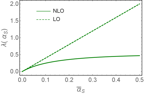
In Fig. 3 we plot , which is the solution to the equation:
| (54) |
This equation is the generalization of Eq. (52) in where we took into account, energy conservation.
Note, that this equation introduces conservation of energy into Eq. (52). The solution to Eq. (54) has the form:
| (55) |
 |
 |
|
| Fig. 3-a | Fig. 3-b |
For the dipole amplitude Eq. (III.4.4) has the following form
| (56) |
For Eq. (56), as well as for Eq. (48), we can find a solution, which is the function of one variable . Indeed, the equation Eq. (56) takes the form
| (57) |
As we have seen in the discussion of Eq. (48), the natural choice of parameters and is and .
Solution: generalities:
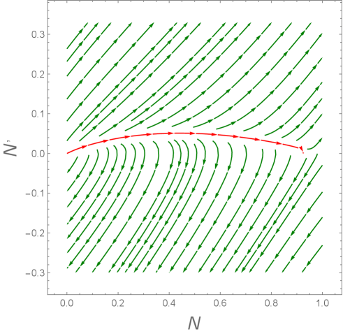
We have not found the explicit solution to Eq. (57). This is the reason for discussing the general features of the solution in this subsection, based on the phase portrait (see Ref.DIFEQ ). The equation can be re-written in the matrix form as
| (58) |
Eq. (58) has two critical points: and . Near these critical points, Eq. (58) can be re-written in the matrix form:
| (59) |
where denotes a small deviation of in the vicinity of the critical point . Matrices have the following forms:
| (60) |
The eigenvalues of these matrices are equal to
| critical point (0,0) | |||||
| critical point (1,0) | (61) |
Therefore, the point (0,0) is the source from which our system originates, while the point (1,0) is a saddle point, since only one of the eigenvalues is negative. Hence, there exist one solution of our equation which gives
| (62) |
The path for this solution in the plane is shown in Fig. 4 by a red line.
Using Eq. (III.4.4), we can find solutions in the vicinity of the critical points. Indeed, at the eigenfunctions of Eq. (59) in the vicinity of the critical point (0,0) have the form:
| (63) |
Therefore, the general solution at has the form
| (64) |
Note that , similarly, at we have in the vicinity of the critical point (1,0):
| (65) |
and
| (66) |
Since in vicinity of the critical point (1,0) is positive, we need to put and therefore, we have
| (67) |
Analytical solutions in the bounded regions:
The previous analysis can be improved in two different kinematic regions: at small , when non-linear corrections are small; and at , where we can develop the semi-classical approach.
Eq. (57) can be solved, by looking for the solution . The equation takes the form:
| (68) |
For the solution of Eq. (68) takes the form:
| (69) |
As we have seen (see Eq. (48) and Eq. (56)), the natural choice of parameters and is, and, , which leads to . The dependence of on can be recovered from the equation:
| (70) |
which has the solution:
| (71) |
with , where
| (72) |
Note that Eq. (71) gives , as a function of (see Eq. (57)) in the vicinity of the saturation scale. As we have discussed, the energy variable leads to the Eq. (III.4.4), and Eq. (20) determines . Therefore, to obtain we need to re-calculate the variable in terms of and : . Hence, in Eq. (71)
| (73) |
with
| (74) |
It should be noted, that Eq. (71) is the same as the solution of Eq. (III.4.4) and Eq. (63), which we obtained in a different way.
In Fig. 5 we plot the dependence on the values of . One can see that Eq. (72) leads to at rather large values of , which is needed for the description of the HERA experimental data
 |
 |
|
| Fig. 5-a | Fig. 5-b |
In the kinematic region, where it is more convenient to solve Eq. (57) directly, by looking for the solution in the form , assuming that is a smooth function of (). For such a function , Eq. (57) can be re-written in the form:
| (75) |
Solving Eq. (75) we obtain
| (76) |
Therefore, can be found from the equation
| (77) |
We choose the sign in Eq. (77) since we are looking for which is positive at large , leading to .
Using Eq. (77) we can evaluate and :
| (78) |
The integral over can be taken then, and Eq. (77)has the form:
| (79) | |||||
where is the initial value of at .
At large , , while at small , . Note, that we obtain similar behaviour of the amplitude at as in Eq. (71), but with a different power of .
In Fig. 6 we plot the solution of Eq. (54). Note, that Fig. 6-c shows that only for . Therefore, for we have to solve the following equation:
| (80) |
 |
 |
 |
| Fig. 6-a | Fig. 6-b | Fig. 6-c |
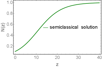
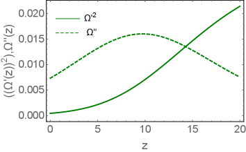
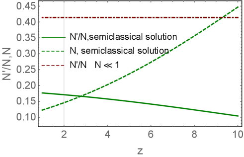
Practical way to obtain estimates for the scattering amplitude:
The difficulties in solving the general equations (see Eq. (57) and Eq. (80)), are that the critical point (1,0) is not a stable point, but only a saddle point. This means that there exists only one path which gives the solution with at large (see Fig. 4). It is difficult to find this trajectory analytically or/and numerically. These difficulties are illustrate by Fig. 7 where and for the semiclassical solution of Eq. (75) are shown in green, while the values of for small , are plotted in red. One can see that it is not possible to find a function which provides a smooth matching to these two solutions. The only possibility is to find the exact solution, that covers a large region of .
III.4.5 Energy conservation in DLA
We need to consider Eq. (18), which follows from Eq. (9) in the region , for taking energy conservation into account. Resolving this equation with respect to we obtain for the amplitude :
| (81) |
which leads to the following equation
| (82) |
instead of Eq. (33). Repeating the same procedure as in section III-C-3, the following non-linear equation can be written:
| (83) |
Neglecting the term in Eq. (83), we have a linear equation which determines the value of the saturation scale and :
| (84) |
Tedious but simple calculations following the procedure of section III-C lead to
| (85) |
The values of and are plotted in Fig. 5-b.
Introducing a new variable , this equation has the form:
IV NLO BFKL kernel in the saturation domain
IV.1 The kernel in -representation
The BFKL kernel of Eq. (3) includes the summation over all twist contributions. In the simplified approach we restrict ourselves to the leading twist term only, which has the formLETU
| (93) |
instead of the full expression of Eq. (3).
In the previous section we specified how we changed the kernel in the perturbative QCD region, taking into account the NLO corrections. We now desire to find how we need to change the kernel for (in the saturation region). For this purpose we re-write Eq. (9) in the vicinity of , where it has the form:
| (94) |
This eigenvalue describes the behaviour of for (see Fig. 3). We start from the simplified expression for Eq. (94):
| (95) |
Resolving Eq. (95) with respect of we obtain
| (96) |
which differs from the behaviour of the LO kernel, only by replacing . Therefore, we can discuss the non-linear equation in the LO, substituting in place of , at the final stage.
IV.2 The non-linear equation
In the saturation region where , the logarithms originate from the decay of a large size dipole, into one small size dipole and one large size dipoleLETU . However, the size of the small dipole is still larger than . This observation can be translated in the following form of the kernel in the LO
| (97) | |||||
where and .
Inside the saturation region the BK equation of the LO takes the form
| (98) |
where .
IV.3 The solution
For solving this equation we introduce function LETU
| (100) |
Substituting Eq. (100) into Eq. (99) we reduce it to the form
| (101a) | |||
| (101b) | |||
where is given by Eq. (72). The variable is defined as
| (102) |
The use of this variable indicates the main idea of our approach: we wish to match the solution of the non-linear Eq. (101b) with the solution of the non-linear Eq. (87). However, we assume that for we need the solution for Eq. (87) for , where it has the form with
| (103) |
and is determined by Eq. (72).
Eq. (101b) has a traveling wave solution (see formula 3.4.1.1 of Ref.MATH ). For Eq. (101b) in the canonical form:
| (104) |
with , the solution takes the form:
| (105) |
where all constants have to be determined from the initial and boundary conditions of Eq. (25). First we see that and . From the condition at we can find . Indeed, differentiating Eq. (105) with respect to one can see that at we have:
| (106) |
From Eq. (106) one can see that choosing
| (107) |
we satisfy the initial condition of Eq. (72).
Finally, the solution of Eq. (105) can be re-written in the following form for :
| (108) |
For and if , Eq. (108) can be solved explicitly giving
| (109) |
Eq. (109) gives the solution which depends only on one variable , and satisfies the initial conditions of Eq. (25).
IV.4 Non-linear equation: NLO + energy conservation
In this section we discuss the general form of the eigenvalues which is given by Eq. (94). We obtain the following solution for from this equation.
| (112) |
where and (see Eq. (34)).
Therefore, the general solution for linear equation takes the form:
| (113) |
One can see that for we have:
| (114) |
with .
We assume that the main contributions stem from the region and/or Bearing this in mind we can use Eq. (97) for the kernel , which can be re-written in the form:
| (115) | |||||
where .
Using Eq. (115) we can re-write the general BK equation (see Eq. (II)) in the form:
| (116) |
Using Eq. (114) we can re-write Eq. (116) in the form:
| (117) |
Introducing we reduce Eq. (117) to the following expression:
| (118) |
Differentiating Eq. (118) with respect to we obtain:
| (119) |
Plugging the last term in Eq. (119) from Eq. (118) we have:
| (120) |
Looking for the solution which has the geometric scaling behaviour, we re-write Eq. (120) in new variable and it takes the form
| (121) |
One can see that deep in the saturation region, where , . However, for we reproduce the solution of Eq. (110). Therefore, we can infer that the energy conservation crucially changed the behaviour of the scattering amplitude deep in the saturation region. In Fig. 8 we plot the solution to Eq. (101b) and to Eq. (121). One can see that the difference is large for . At , which corresponds the kinematic region of HERA, this difference is not so large and can be neglected.
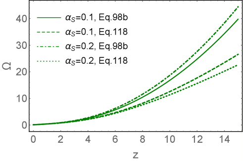
However, accounting of energy conservation is beyond the NLOBK, which is the subject of this paper. We believe, that it is necessary to find the corrections of next-to-next-to leading order to treat the energy conservation on a theoretical footing.
V Conclusions
Concluding, we wish to formulate clearly the three stages of our approach:
-
1.
For (perturbative QCD region) we suggest to use the linear evolution equation(see Eq. (56):
(122) We have discussed this equation in the section III-D-4. Recalling that in the derivation of this equation we use the DLA in which both and are considered to be large: . For () we can use the experimental data as the initial condition for Eq. (122). The value of the saturation momentum is given by Eq. (III.4.5). Since its value turns out to be much less than , which stems from the condition = , we can use the DGLAP evolution equation in the next-to-leading order for .
- 2.
-
3.
For (saturation region), we propose to use the solution to the non-linear equation which has the following form:
(124) This equation does not take into account the corrections relating to energy conservation, but it is simple, and for large region of the solution to the non-linear equation of section IV-D-1, is described quite well by Eq. (124).
In general, we developed the approach based on the DLA approximation of perturbative QCD, and on the non-linear evolution for the leading twist approximation. We considered the non-linear equations, which arise in different kinematic regions , and discussed solutions to them.
We believe that our suggested approach which takes into account the main features of the NLO corrections to the BFKL kernel, and which is likely to describe the experimental data for DIS processes. Indeed, Fig. 5-b shows that the energy dependence of the saturation scale, as well as the value of , are very close to the values that stem from saturation models, that describe the data quite well (see Ref.RESH for example).
VI Acknowledgements
We thank our colleagues at Tel Aviv university and UTFSM for encouraging discussions. Our special thanks go to E. Gotsman for all his remarks and suggestions on this paper. This research was supported by ANID PIA/APOYO AFB180002 (Chile), Fondecyt (Chile) grants 1180118 and 1191434, Conicyt Becas (Chile) and PIIC 20/2020, DPP, Universidad Técnica Federico Santa María.
References
- (1) Yuri V Kovchegov and Eugene Levin, “ Quantum Choromodynamics at High Energies", Cambridge Monographs on Particle Physics, Nuclear Physics and Cosmology, Cambridge University Press, 2012 .
- (2) J. Jalilian-Marian, A. Kovner, A. Leonidov, and H. Weigert, “The BFKL equation from the Wilson renormalization group" , Nucl. Phys. B504 (1997) 415–431, [ arXiv:hep-ph/9701284].
- (3) J. Jalilian-Marian, A. Kovner, A. Leonidov, and H. Weigert, “The Wilson renormalization group for low x physics: Towards the high density regime" , Phys.Rev. D59 (1998) 014014, [arXiv:hep-ph/9706377 [hep-ph]].
- (4) A. Kovner, J. G. Milhano, and H. Weigert, “Relating different approaches to nonlinear QCD evolution at finite gluon density" , Phys. Rev. D62 (2000) 114005, [ arXiv:hep-ph/0004014].
- (5) E. Iancu, A. Leonidov, and L. D. McLerran, Nonlinear gluon evolution in the color glass condensate. I" ,Nucl. Phys. A692 (2001) 583–645, [ arXiv:hep-ph/0011241].
- (6) E. Iancu, A. Leonidov, and L. D. McLerran, “The renormalization group equation for the color glass condensate" , Phys. Lett. B510 (2001) 133–144, [ arXiv:hep-ph/0102009].
- (7) I. Balitsky, “Operator expansion for high-energy scattering", [arXiv:hep-ph/9509348]; “Factorization and high-energy effective action", Phys. Rev. D60, 014020 (1999) [arXiv:hep-ph/9812311]; Y. V. Kovchegov, “ Small-x structure function of a nucleus including multiple Pomeron exchanges"’ Phys. Rev. D60, 034008 (1999), [arXiv:hep-ph/9901281].
- (8) E. Ferreiro, E. Iancu, A. Leonidov, and L. McLerran, “Nonlinear gluon evolution in the color glass condensate. II" , Nucl. Phys. A703 (2002) 489–538, [ arXiv:hep-ph/0109115].
- (9) V. S. Fadin, E. A. Kuraev and L. N. Lipatov, “On the pomeranchuk singularity in asymptotically free theories", Phys. Lett. B60, 50 (1975); E. A. Kuraev, L. N. Lipatov and V. S. Fadin, “The Pomeranchuk Singularity in Nonabelian Gauge Theories" Sov. Phys. JETP 45, 199 (1977), [Zh. Eksp. Teor. Fiz.72,377(1977)]; I. I. Balitsky and L. N. Lipatov,“The Pomeranchuk Singularity in Quantum Chromodynamics,” Sov. J. Nucl. Phys. 28, 822 (1978), [Yad. Fiz.28,1597(1978)].
- (10) L. N. Lipatov, “Small x physics in perturbative QCD,” Phys. Rept. 286, 131 (1997) [hep-ph/9610276]; “The Bare Pomeron in Quantum Chromodynamics,” Sov. Phys. JETP 63, 904 (1986) [Zh. Eksp. Teor. Fiz. 90, 1536 (1986)].
- (11) I. Balitsky, “Quark contribution to the small-x evolution of color dipole,” Phys. Rev. D 75 (2007) 014001, [hep-ph/0609105].
- (12) Y. V. Kovchegov and H. Weigert, “Triumvirate of Running Couplings in Small-x Evolution,” Nucl. Phys. A 784 (2007) 188, [hep-ph/0609090].
- (13) I. Balitsky and G. A. Chirilli, “Next-to-leading order evolution of color dipoles", Phys.Rev. D77 (2008) 014019, [arXiv:0710.4330 [hep-ph]].
- (14) I. Balitsky and G. A. Chirilli, “Rapidity evolution of Wilson lines at the next-to-leading order", Phys.Rev. D88 (2013) 111501, [ arXiv:1309.7644 [hep-ph]].
- (15) A. Kovner, M. Lublinsky, and Y. Mulian, “Jalilian-Marian, Iancu, McLerran, Weigert, Leonidov, Kovner evolution at next to leading order", Phys.Rev. D89 (2014) no. 6, 061704, [ arXiv:1310.0378 [hep-ph]].
- (16) A. Kovner, M. Lublinsky, and Y. Mulian, “NLO JIMWLK evolution unabridged", JHEP 08 (2014) 114, [ arXiv:1405.0418 [hep-ph]].
- (17) M. Lublinsky and Y. Mulian, “High Energy QCD at NLO: from light-cone wave function to JIMWLK evolution", JHEP 05 (2017) 097, [arXiv:1610.03453 [hep-ph]].
- (18) B. Duclou, E. Iancu, A. H. Mueller, G. Soyez and D. N. Triantafyllopoulos, “Non-linear evolution in QCD at high-energy beyond leading order,” JHEP 1904 (2019) 081 doi:10.1007/JHEP04(2019)081 [arXiv:1902.06637 [hep-ph]] and references therein.
- (19) V. S. Fadin and L. N. Lipatov, “BFKL pomeron in the next-to-leading approximation,” Phys. Lett. B 429 (1998) 127 [hep-ph/9802290].
- (20) M. Ciafaloni and G. Camici, “Energy scale(s) and next-to-leading BFKL equation,” Phys. Lett. B 430 (1998) 349 [hep-ph/9803389].
- (21) G. P. Salam, “A Resummation of large subleading corrections at small x,” JHEP 9807 (1998) 019 doi:10.1088/1126-6708/1998/07/019 [hep-ph/9806482];
- (22) M. Ciafaloni, D. Colferai and G. P. Salam, “Renormalization group improved small equation,” Phys. Rev. D 60 (1999) 114036 doi:10.1103/PhysRevD.60.114036 [hep-ph/9905566].
- (23) M. Ciafaloni, D. Colferai, G. P. Salam and A. M. Stasto, “Renormalization group improved small Green’s function,” Phys. Rev. D 68 (2003) 114003, [hep-ph/0307188].
- (24) E. Levin and K. Tuchin, “Solution to the evolution equation for high parton density QCD,” Nucl. Phys. B 573, 833 (2000) [hep-ph/9908317]; “New scaling at high-energy DIS,” Nucl. Phys. A 691, 779 (2001) [hep-ph/0012167]; “Nonlinear evolution and saturation for heavy nuclei in DIS,” 693, 787 (2001) [hep-ph/0101275].
- (25) L. V. Gribov, E. M. Levin and M. G. Ryskin, “Semihard Processes in QCD,” Phys. Rept. 100 (1983) 1.
- (26) A. H. Mueller and J. Qiu, “Gluon recombination and shadowing at small values of ", Nucl. Phys. B268 (1986) 427
- (27) L. McLerran and R. Venugopalan, “Computing quark and gluon distribution functions for very large nuclei", Phys. Rev. D49 (1994) 2233, “Gluon distribution functions for very large nuclei at small transverse momentum", Phys. Rev. D49 (1994), 3352; ‘Green?s function in the color field of a large nucleus", D50 (1994) 2225; “ Fock space distributions, structure functions, higher twists, and small " , D59 (1999) 09400.
- (28) V. A. Khoze, A. D. Martin, M. G. Ryskin and W. J. Stirling, “The spread of the gluon -distribution and the determination of the saturation scale at hadron colliders in resummed NLL BFKL,” Phys. Rev. D 70 (2004) 074013 [hep-ph/0406135].
- (29) A. Sabio Vera, “An ’All-poles’ approximation to collinear resummations in the Regge limit of perturbative QCD,” Nucl. Phys. B 722, 65-80 (2005) doi:10.1016/j.nuclphysb.2005.06.003 [arXiv:hep-ph/0505128 [hep-ph]].
- (30) J. Bartels, E. Levin, “Solutions to the Gribov-Levin-Ryskin equation in the nonperturbative region,” Nucl. Phys. B387 (1992) 617-637;
- (31) A. H. Mueller and D. N. Triantafyllopoulos, “The Energy dependence of the saturation momentum,” Nucl. Phys. B 640 (2002) 331 [hep-ph/0205167]
- (32) E. Iancu, K. Itakura and L. McLerran, “Geometric scaling above the saturation scale,” Nucl. Phys. A 708 (2002) 327 [hep-ph/0203137].
- (33) A. M. Stasto, K. J. Golec-Biernat, J. Kwiecinski, “Geometric scaling for the total gamma* p cross-section in the low x region,” Phys. Rev. Lett. 86 (2001) 596-599, [hep-ph/0007192].
- (34) C. Contreras, E. Levin and R. Meneses, “BFKL equation in the next-to-leading order: solution at large impact parameters,” Eur. Phys. J. C 79 (2019) no.10, 842 [arXiv:1906.09603 [hep-ph]].
- (35) I. Gradstein and I. Ryzhik, Table of Integrals, Series, and Products, Fifth Edition, Academic Press, London, 1994.
- (36) Morris W. Hirsch, Stephen Smale and Robert L. Devaney,“Differential Equations, Dynamical Systems, and an Introduction to Chaos", 3rd Edition,Academic Press, 2013.
- (37) A.D. Polyanin and V.F. Zaitsev “Handbook of nonlinear partial differential equations", Chapman and Hall/CRC Press, 2004, Raca Baton, New York, London, Tokyo.
- (38) C. Contreras, E. Levin, R. Meneses and I. Potashnikova, “CGC/saturation approach: a new impact-parameter dependent model in the next-to-leading order of perturbative QCD,” Phys. Rev. D 94 (2016) no.11, 114028 doi:10.1103/PhysRevD.94.114028 [arXiv:1607.00832 [hep-ph]].
- (39) W. Xiang, Y. Cai, M. Wang and D. Zhou, “Rare fluctuations of the -matrix at NLO in QCD,” Phys. Rev. D 99 (2019) no.9, 096026 doi:10.1103/PhysRevD.99.096026 [arXiv:1812.10739 [hep-ph]].
- (40) A. H. Rezaeian and I. Schmidt, “Impact-parameter dependent Color Glass Condensate dipole model and new combined HERA data,” Phys. Rev. D 88 (2013) 074016 [arXiv:1307.0825 [hep-ph]].